A Static Spherically Symmetric Solution of the Einstein-aether Theory

Abstract

By using of the Euler-Lagrange equations, we find a static spherically symmetric solution in the Einstein-aether theory with the coupling constants restricted. The solution is similar to the Reissner-Nordstrom solution in that it has an inner Cauchy horizon and an outer black hole event horizon. But a remarkable difference from the Reissner-Nordstrom solution is that it is not asymptotically flat but approaches a two dimensional sphere. The resulting electric potential is regular in the whole spacetime except for the curvature singularity. On the other hand, the magnetic potential is divergent on both Cauchy horizon and the outer event horizon.

I Introduction

The Einstein-aether theory ted:00 ; ted:07 belongs to the vector-tensor theories in nature. Besides the ordinary matters and the metric tensor $g_{\mu\nu}$, the fundamental field in the theory is a timelike vector field $A_{\mu}$. Different from the usual vector-tensor theories, $A_{\mu}$ is constrained to have a constant norm. So the vector field $A_{\mu}$ cannot vanish anywhere. Therefore, a preferred frame is defined and the Lorentz symmetry is violated. The vector field is referred to as the “aether”. The Einstein-aether theory has become an interesting theoretical laboratory to explore both the Lorentz violation effects and the preferred frame effects. Up to now, the Einstein-aether theory has been widely studied in literature in various ways: the analysis of classical and quantum perturbations lim:05 ; na:10 ; car:00 ; car:01 ; car:02 ; car:03 , the cosmologies car:04 ; bon:08 , the gravitational collapse gar:08 , the Einstein-aether waves wave:04 , the radiation damping fos:06 and so on.

The purpose of the present paper is to seek for a static spherically symmetric solution of the Einstein-aether theory. The black hole solutions in the Einstein-aether theory have been investigated in Refs. bh1 ; bh2 ; bh3 ; bh4 ; bh5 . These investigations mainly focus on the numerical analysis of the solutions due to the complication of the Einstein equations. To our knowledge, one have not yet find the exact, static and spherically symmetric solution in the Einstein-aether theory. In this paper, instead of solving the Einstein equations, we are going to solve the Euler-Lagrange equations in order to derive the static spherically symmetric solution. We find it is relatively simple in the calculations. We shall use the system of units in which $16\pi G=c=\hbar=4\pi\varepsilon_{0}=1$ and the metric signature $(-,\ +,\ +,\ +)$ throughout the paper.

II static spherically symmetric solution

In the context of spherical symmetry and after the redefinitions of metric $g_{\mu\nu}$ and aether field $A_{\mu}$, the Lagrangian density of the Einstein-aether theory can be written as

$$\mathscr{L} = -R-\frac{c_{1}}{2}F_{\mu\nu}F^{\mu\nu}-c_{2}\left(\nabla_{\mu}A^{\mu}\right)^{2}+\lambda\left(A_{\mu}A^{\mu}+m^{2}\right)\;,$$ (1)

with the field strength tensor

$$F_{\mu\nu} = \nabla_{\mu}A_{\nu}-\nabla_{\nu}A_{\mu}\;.$$ (2)

Here $R$ is the Ricci scalar and the $c_{i}$ are dimensionless constants. We note that there is a sign difference from gar:08 in the definition of Ricci tensor. $\lambda$ is the Lagrange multiplier field which has the dimension of the square of inverse length, $l^{-2}$. $m$ is a positive dimensionless constant which has the physical meaning of the squared norm for the aether field. The requirement of $m^{2}>0$ ensures the aether to be timelike.

The static and spherically symmetric metric can always be written as

$$ds^{2}=-U\left(r\right)dt^{2}+\frac{1}{U\left(r\right)}dr^{2}+f\left(r\right)^{2}d\Omega^{2}\;.$$ (3)

Instead of solving the Einstein equations, we prefer to deal with the Euler-Lagrange equations from the Lagrangian Eq. (1) for simplicity in calculations. Because of the static and spherically symmetric property of the spacetime, the vector field $A_{\mu}$ takes the form

$$A_{\mu}=\left[\phi\left(r\right),\ \frac{1}{\psi\left(r\right)},\ 0,\ 0\right]\;,$$ (4)

where $\phi$ and $\psi^{-1}$ correspond to the electric and magnetic part of the electromagnetic potential. Then we have

$$F_{\mu\nu}F^{\mu\nu}=-2\phi^{{}^{\prime}2}\;,\ \ \ \nabla_{\mu}A^{\mu}=\left(\frac{U}{\psi}\right)^{{}^{\prime}}+2\frac{f^{{}^{\prime}}U}{f\psi}\;.$$ (5)

The prime here and in what follows denotes the derivative with respect to $r$. Taking into account the Ricci scalar, $R$, we have the total Lagrangian as follows

$$\mathscr{L} = -U^{{}^{\prime\prime}}-4U^{{}^{\prime}}\frac{f^{{}^{\prime}}}{f}-4U\frac{f^{{}^{\prime\prime}}}{f}+\frac{2}{f^{2}}-2U\frac{f^{{}^{\prime}2}}{f^{2}}$$ (6)

$$+{c_{1}}\phi^{{}^{\prime}2}-c_{2}\left[\left(\frac{U}{\psi}\right)^{{}^{\prime}}+2\frac{f^{{}^{\prime}}U}{f\psi}\right]^{2}$$

$$+\lambda\left(-\frac{1}{U}\phi^{2}+\frac{U}{\psi^{2}}+m^{2}\right)\;.$$

Let

$$\psi=\frac{Uf^{2}}{K}\;,$$ (7)

we can rewrite the Lagrangian, Eq. (6), as follows

$$\mathscr{L} = -U^{{}^{\prime\prime}}-4U^{{}^{\prime}}\frac{f^{{}^{\prime}}}{f}-4U\frac{f^{{}^{\prime\prime}}}{f}+\frac{2}{f^{2}}-2U\frac{f^{{}^{\prime}2}}{f^{2}}$$ (8)

$$+{c_{1}}\phi^{{}^{\prime}2}-c_{2}\frac{K^{{}^{\prime}2}}{f^{4}}$$

$$+\lambda\left(-\frac{1}{U}\phi^{2}+\frac{K^{2}}{Uf^{4}}+m^{2}\right)\;.$$

Now there are $U,\ f,\ \phi,\ K,\ \lambda$ five variables in the Lagrangian which correspond to five equations of motion. Then using the Euler-Lagrange equation, we obtain the equation of motion for $\lambda$,

$$-\frac{1}{U}\phi^{2}+\frac{K^{2}}{Uf^{4}}+m^{2}=0\;,$$ (9)

for $\phi$,

$$c_{1}Uf\phi^{{}^{\prime\prime}}+2c_{1}U\phi^{{}^{\prime}}f^{{}^{\prime}}+\lambda\phi f=0\;,$$ (10)

for $K$,

$$c_{2}UfK^{{}^{\prime\prime}}-2c_{2}UK^{{}^{\prime}}f^{{}^{\prime}}+\lambda Kf=0\;,$$ (11)

for $U$,

$$-2U^{2}f^{3}f^{{}^{\prime\prime}}-\lambda K^{2}+\lambda\phi^{2}f^{4}=0\;,$$ (12)

and for$f$,

$$-c_{1}\phi^{{}^{\prime}2}Uf^{4}-c_{2}UK^{{}^{\prime}2}+\lambda\phi^{2}f^{4}+Uf^{4}U^{{}^{\prime\prime}}-\lambda m^{2}Uf^{4}$$

$$+2Uf^{3}U^{{}^{\prime}}f^{{}^{\prime}}+2U^{2}f^{3}f^{{}^{\prime\prime}}+\lambda K^{2}=0\;,$$ (13)

respectively. We have five independent differential equations and five variables, $U,\ f,\ \phi,\ K,\ \lambda$. So the system of equations is closed.

From Eq. (9) and Eq. (56), we obtain

$$U=\frac{\phi^{2}f^{4}-K^{2}}{m^{2}f^{4}}\;,$$ (14)

and

$$\lambda=-\frac{c_{1}U\left(f\phi^{{}^{\prime\prime}}+2\phi^{{}^{\prime}}f^{{}^{\prime}}\right)}{f\phi}\;,$$ (15)

respectively. Substituted Eq. (14) and Eq. (15) into Eq. (12), then Eq. (12) becomes

$$2\phi f^{{}^{\prime\prime}}+c_{1}m^{2}f\phi^{{}^{\prime\prime}}+2c_{1}m^{2}\phi^{{}^{\prime}}f^{{}^{\prime}}=0\;.$$ (16)

The norm of the aether field is usually constrained by the Lagrange multiplier to be unity, $m=1$. But in this paper, we would constrain the norm to meet

$$c_{1}m^{2}=2\;.$$ (17)

We note that this choice is consistent with the perturbation analysis of Lim lim:05 . He showed that in order to have a positive definite Hamiltonian, $c_{1}$ should satisfy

$$c_{1}>0\;.$$ (18)

We stress that the choice of $c_{1}m^{2}=2$ corresponds to the special case that has been called $c_{14}=2$ eling04 ; car:04 which leads the Newton’s gravitational constant to infinityeling04 ; car:04 :

$$G_{N}=\frac{G}{1-c_{14}/2}\;.$$ (19)

But Eq. (19) should be taken with a grain of salt because it is derived with vanishing spatial components in $A^{\mu}$. We also stress that the choice of $c_{1}m^{2}=2$ is not “ for convenience ” but actually a restriction on the theory .

Then Eq. (16) gives the solution as follows

$$\phi=\frac{\phi_{0}+\phi_{1}r}{f}\;,$$ (20)

where $\phi_{0},\ \phi_{1}$ are two integration constants. $\phi_{1}$ is dimensionless while $\phi_{0}$ has the dimension of length.

Keeping Eqs. (14), (15) and (20) in mind, we find Eq.(11) and Eq. (II) are reduced to the following form

$$2c_{2}m^{2}K^{{}^{\prime}}f^{{}^{\prime}}-c_{2}m^{2}fK^{{}^{\prime\prime}}-2Kf^{{}^{\prime\prime}}=0\;,$$ (21)

and

$$2f^{2}K^{{}^{\prime}2}+12K^{2}f^{{}^{\prime}2}-12fKf^{{}^{\prime}}K^{{}^{\prime}}+c_{2}m^{2}f^{2}K^{{}^{\prime}2}$$

$$-6fK^{2}f^{{}^{\prime\prime}}+2Kf^{2}K^{{}^{\prime\prime}}=0\;,$$ (22)

respectively. Putting

$$c_{2}=\frac{1}{\alpha m^{2}}\;,$$ (23)

with $\alpha$ a new dimensionless parameter, we obtain from Eq. (21) and Eq. (II)

$$6\alpha fK^{2}f^{{}^{\prime\prime}}-12\alpha K^{2}f^{{}^{\prime}2}+8\alpha fKf^{{}^{\prime}}K^{{}^{\prime}}$$

$$+4\alpha^{2}fK^{2}f^{{}^{\prime\prime}}-2\alpha f^{2}K^{{}^{\prime}2}-f^{2}K^{{}^{\prime}2}=0\;.$$ (24)

In order that the spin-$0$ field does not propagate superluminally, Lim constrained $c_{2}$ to meet lim:05

$$c_{2}>0\;,\ \ \ \ \textrm{and}\ \ \ \frac{c_{2}}{c_{1}}\leq 1\;.$$ (25)

Taking account of Eq. (18), we conclude that $\alpha$ should satisfy

$$\alpha\geq\frac{1}{2}\;.$$ (26)

Solving the differential equation, we obtain

$$K=K_{0}\exp\left\{{\int\frac{1}{\left(1+2\alpha\right)f}\left[4\alpha f^{{}^{\prime}}+\sqrt{2\alpha\left(2\alpha+3\right)\left(2\alpha ff^{{}^{\prime\prime}}+ff^{{}^{\prime\prime}}-2f^{{}^{\prime}2}\right)}\right]dr}\right\}\;,$$ (27)

where $K_{0}$ is an integration constant which has the dimension of the square of the length, $l^{2}$. We may assume $K_{0}>0$. Substituting Eq. (27) into Eq. (II), we obtain

$$\left(16\alpha ff^{{}^{\prime\prime}}+8ff^{{}^{\prime\prime}}-16f^{{}^{\prime}2}\right)\sqrt{\alpha\left(2\alpha+3\right)\left(2\alpha ff^{{}^{\prime\prime}}+ff^{{}^{\prime\prime}}-2f^{{}^{\prime}2}\right)}$$

$$+\sqrt{2}\left(4\alpha^{2}f^{2}f^{{}^{\prime\prime\prime}}+12\alpha^{2}ff^{{}^{\prime}}f^{{}^{\prime\prime}}-8\alpha f^{{}^{\prime}3}+4\alpha f^{2}f^{{}^{\prime\prime\prime}}-12\alpha ff^{{}^{\prime}}f^{{}^{\prime\prime}}-9ff^{{}^{\prime}}f^{{}^{\prime\prime}}+f^{2}f^{{}^{\prime\prime\prime}}+12f^{{}^{\prime}3}\right)=0\;.$$ (28)

At first glance, Eq. (II) is rather complicated. But using the calling sequence of “dsolve” in Maple Program, it is easy to find the solutions with $\alpha=1/2,\ \ \alpha=3/2,\ \ \alpha=5/2,\ \cdot\cdot\cdot$. For general $\alpha$, $f$ is found to be

$$f=f_{0}\left(1-k^{2}r^{2}\right)^{\frac{2\alpha+1}{4\alpha-2}}e^{\frac{\sqrt{6\alpha+4\alpha^{2}}}{2\alpha-1}\tanh^{-1}kr}\;,$$ (29)

where $f_{0}$ and $k$ are integration constants. Both $f_{0}$ and $k^{-1}$ have the dimension of length. Without the loss of generality, the third integration constant with the dimension of length has been absorbed by $r$.

Eq. (29) forces $kr$ to satisfy

$$-1\leq kr\leq 1\;.$$ (30)

Up to this point, we could present all the variables:

$$f = f_{0}\left(1-k^{2}r^{2}\right)^{\frac{2\alpha+1}{4\alpha-2}}e^{\frac{\sqrt{6\alpha+4\alpha^{2}}}{2\alpha-1}\tanh^{-1}kr}\;,$$ (31)

$$K = K_{0}\left(1-kr\right)^{\frac{4\alpha-\sqrt{2\alpha\left(2\alpha+3\right)}}{4\alpha-2}}\cdot\left(1+kr\right)^{\frac{4\alpha+\sqrt{2\alpha\left(2\alpha+3\right)}}{4\alpha-2}}\;,$$ (32)

$$\phi = \frac{1}{f_{0}}\left(\phi_{0}+\phi_{1}r\right)\left(1-k^{2}r^{2}\right)^{-\frac{2\alpha+1}{4\alpha-2}}e^{-\frac{\sqrt{6\alpha+4\alpha^{2}}}{2\alpha-1}\tanh^{-1}kr}\;,$$ (33)

$$U = \frac{1}{m^{2}f_{0}^{2}}\left(\phi_{0}+\phi_{1}r\right)^{2}\left(1-k^{2}r^{2}\right)^{-\frac{2\alpha+1}{2\alpha-1}}e^{-\frac{2\sqrt{6\alpha+4\alpha^{2}}\tanh^{-1}kr}{2\alpha-1}}$$ (34)

$$-\frac{K_{0}^{2}}{m^{2}f_{0}^{4}}\left(1-kr\right)^{\frac{4\alpha-\sqrt{2\alpha\left(2\alpha+3\right)}}{2\alpha-1}}\cdot\left(1+kr\right)^{\frac{4\alpha+\sqrt{2\alpha\left(2\alpha+3\right)}}{2\alpha-1}}\left(1-k^{2}r^{2}\right)^{-\frac{4\alpha+2}{2\alpha-1}}e^{-\frac{4\sqrt{6\alpha+4\alpha^{2}}\tanh^{-1}kr}{2\alpha-1}}\;,$$

$$\psi = \frac{\left(\phi_{0}+\phi_{1}r\right)^{2}\left(1-k^{2}r^{2}\right)^{-\frac{4\alpha+\sqrt{6\alpha+4\alpha^{2}}}{4\alpha-2}}\left(1-kr\right)^{\frac{\sqrt{6\alpha+4\alpha^{2}}}{2\alpha-1}}}{K_{0}m^{2}}$$ (35)

$$-\frac{K_{0}\left(1-kr\right)^{\frac{4\alpha}{2\alpha-1}}\left(1+kr\right)^{\frac{4\alpha+\sqrt{6\alpha+4\alpha^{2}}}{2\alpha-1}}}{m^{2}f_{0}^{2}\left(1-k^{2}r^{2}\right)^{\frac{2+8\alpha+\sqrt{6\alpha+4\alpha^{2}}}{4\alpha-2}}e^{\frac{2\sqrt{6\alpha+4\alpha^{2}}\tanh^{-1}kr}{2\alpha-1}}}\;,$$

$$\lambda = -\frac{2k^{2}\left(\phi_{0}+\phi_{1}r\right)^{2}}{f_{0}^{2}m^{4}\left(2\alpha-1\right)^{2}\left(1-k^{2}r^{2}\right)^{\frac{6\alpha-1}{2\alpha-1}}}\left[4kr\sqrt{4\alpha^{2}+6\alpha}-6\alpha-2k^{2}r^{2}-1-4\alpha k^{2}r^{2}\right]e^{-\frac{2\sqrt{6\alpha+4\alpha^{2}}\tanh^{-1}kr}{2\alpha-1}}$$ (36)

$$+\frac{2k^{2}K_{0}^{2}}{f_{0}^{4}m^{4}\left(2\alpha-1\right)^{2}\left(1-k^{2}r^{2}\right)^{\frac{6\alpha-1}{2\alpha-1}}}\left[4kr\sqrt{4\alpha^{2}+6\alpha}-6\alpha-2k^{2}r^{2}-1-4\alpha k^{2}r^{2}\right]$$

$$\cdot\left(1-kr\right)^{\frac{4\alpha-\sqrt{2\alpha\left(2\alpha+3\right)}}{2\alpha-1}}\cdot\left(1+kr\right)^{\frac{4\alpha+\sqrt{2\alpha\left(2\alpha+3\right)}}{2\alpha-1}}e^{-\frac{4\sqrt{6\alpha+4\alpha^{2}}\tanh^{-1}kr}{2\alpha-1}}\;.$$

If we define

$$\phi_{0}\equiv\alpha_{0}f_{0}\;,\ \ \ \phi_{1}\equiv\alpha_{1}\;,\ \ \ k\equiv\alpha_{2}\frac{1}{f_{0}}\;,\ \ \ K_{0}\equiv\alpha_{3}f_{0}^{2}\;,$$ (37)

then $\alpha_{i}$ are dimensionless constants. Together with $m$ and $\alpha$, we have totally six dimensionless constants and one dimensional parameter, $f_{0}$. We note that the seven parameters are not independent and there are six parameters in the solution in nature. In fact, Eling and Jacobson  bh3 have argued that there is a $3$-parameter (corresponding to the mass, electric charge and magnetic charge, respectively) family of spherical, static solutions before asymptotic flatness and regularity are imposed. If one take into account the two coupling constants, that would be $5$ parameters in all. But our solution Eqs. (31-36) is not asymptotic flat. So there is an extra parameter of “cosmological-constant-like”. Then the total number of parameters is six. This could be understood from the expression of $f$ and $U$ with the replacements

$$\frac{\phi_{0}}{mf_{0}}\rightarrow\bar{\phi_{0}}\;,\ \ \ \frac{\phi_{1}}{mf_{0}}\rightarrow\bar{\phi_{1}}\;,\frac{K_{0}}{mf_{0}^{2}}\rightarrow\bar{K_{0}}\;.$$ (38)

Then the metric of spacetime is determined by six parameters.

III structure of the spacetime

In this section, let’s numerically study the structure of spacetime described by the solution. Since $f$ is the physical length, we should rewrite the metric as follows

$$ds^{2}=-U\left(r\right)dt^{2}+\frac{1}{V\left(r\right)}df^{2}+f\left(r\right)^{2}d\Omega^{2}\;,$$ (39)

with

$$V\left(r\right)={U\left(r\right)f^{{}^{\prime}2}}\;.$$ (40)

Now $f$ plays the role of physical radius (proper length) of the static spherically symmetric space.

As an example, we put the dimensional constant $f_{0}=1$(for example, $f_{0}$ equals to one Schwarzschild radius). Five dimensionless constants are put $m=1,\ \alpha_{0}=\alpha_{2}=1,\ \ \alpha=3/2$. As for $\alpha_{1}$, we let $\alpha_{1}=0.15,\ 0.1,\ 0,\ -0.2,\ -0.4$, respectively.

There are usually two kinds of horizons in a static spherically symmetric spacetime, namely, the timelike limit surface (TLS) and the event horizon (EH). The timelike limit surface separates the timelike region of the Killing vector field from the spacelike part which is determined by Haw73

$$g_{00}=U=0\;.$$ (41)

In Fig. 1, we plot the evolution of $U$ with respect to the physical radius $\ln f$ for different $\alpha_{1}$. The figure shows that there are two TLS in the spacetime in general. One of them is the inner Cauchy horizon and the other is the black hole event horizon. This is very similar to the spacetime of Reissner-Nordstrom solution. On the other hand, the Reissner-Nordstrom spacetime is asymptotically flat in space. But this solution is asymptotically a two dimensional sphere. With the increasing of $\alpha_{1}$, the event horizon is shrinking. When $\alpha_{1}=0$, the inner Cauchy horizon and the black hole event horizon coincide and the solution corresponds to the extreme solution.

Compared to Fig. 1, the structure of Reissner-Nordstrom spacetime is shown in Fig. 2. The metric of Reissner-Nordstrom spacetime takes the form of

$$ds^{2} = -Udt^{2}+\frac{1}{U}df^{2}+f^{2}d\Omega^{2}\;,\ \ \ \$$

$$U = 1-\frac{2M}{f}+\frac{Q^{2}}{f^{2}}\;.$$ (42)

Without the loss of generality, we take the mass $M=1.0$ and the electric charge $Q=1.3,\ 1.0,\ 0.8,\ 0.7$, respectively. There are two horizons in the spacetime, the inner Cauchy horizon (CH) and the black hole event horizon (EH). (As an example, the CH and EH are given for $Q=0.7$). The space is asymptotically flat. With the increasing of electric charge $Q$, the EH is shrinking and the CH expanding. When $Q=M=1.0$, the inner Cauchy horizon and the black hole event horizon coincide and the solution corresponds to the extreme solution.

On the other hand, the EH is determined by Haw73

$$g^{11}=V=0\;.$$ (43)

In Fig. 3, we plot the evolution of $V$ with respect to the physical radius $\ln f$ for different $\alpha_{1}$. The figure shows that there are two horizons in the spacetime in general, namely, the inner Cauchy horizon and the black hole event horizon. With the increasing of $\alpha_{1}$, the event horizon is shrinking. When $\alpha_{1}=0$, the inner Cauchy horizon and the black hole event horizon coincide and the solution corresponds to the extreme solution.

In Fig. 4, we plot the evolution of the electric potential $\phi$ with respect to the physical radius $f$ for different $\alpha_{1}$. It shows that $\phi$ is regular in the spacetime except for $f=0$ (curvature singularity). The potential $\phi$ is divergent at $f=0$ and asymptotically approaches zero in the infinity of space. This behavior is the same as the electric potential in Reissner-Nordstrom solution.

In order to show $f=0$ is the curvature singularity, as an example, we plot the evolution of the Ricci scalar $R$ with respect to the physical radius $f$ in Fig. 5 with $m=1,\ \alpha_{0}=\alpha_{2}=1,\ \ \alpha=3/2,\ \ \ \alpha_{1}=-0.4$. It is apparent $R$ is divergent at $f=0$. This reveals $f=0$ is indeed the curvature singularity.

In Fig. 6, we plot the evolution of the inverse of magnetic potential $\psi$ with respect to the physical radius $\ln f$ for different $\alpha_{1}$. It shows that the magnetic potential $\psi^{-1}$ is divergent on both horizons while asymptotically approaches zero in both the infinity of space and the curvature singularity.

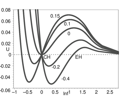
Figure 1: The evolution of $U$ with respect to the physical radius $\ln{f}$ for different $\alpha_{1}=-0.4,\ -0.2,\ 0,\,0.1,\ 0.15$. There are two horizons in the spacetime in general, the inner Cauchy horizon (CH) and the black hole event horizon (EH) (As an example, the CH and EH are given for $\alpha_{1}=-0.4$). When $f\rightarrow\infty$, we have $U=0$. So the solution is not asymptotically flat in space. With the increasing of $\alpha_{1}$, the event horizon is shrinking. When $\alpha_{1}=0$, the inner Cauchy horizon and the black hole event horizon coincide and the solution corresponds to the extreme solution.

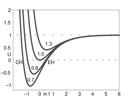
Figure 2: The evolution of $U$ with respect to the physical radius ${f}$ in the Reissner-Nordstrom solution for different electric charge $Q=1.3,\ 1.0,\ 0.8,\ 0.7$. There are two horizons in the spacetime, the inner Cauchy horizon (CH) and the black hole event horizon (EH). (As an example, the CH and EH are given for $Q=0.7$). The space is asymptotically flat. With the increasing of electric charge $Q$, the EH is shrinking and the CH expanding. When $Q=M=1.0$, the inner Cauchy horizon and the black hole event horizon coincide and the solution corresponds to the extreme solution.

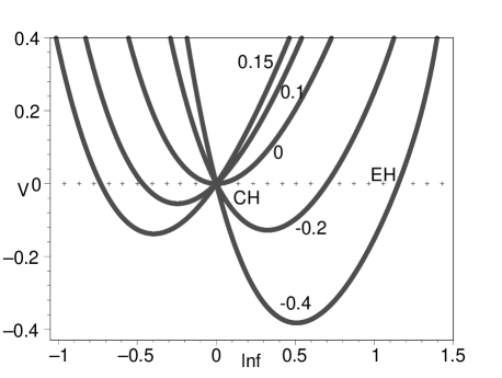
Figure 3: The evolution of $V$ with respect to the physical radius $\ln{f}$ for different $\alpha_{1}=-0.4,\ -0.2,\ 0,\,0.1,\ 0.15$. There are two horizons in the spacetime in general, the inner Cauchy horizon and the black hole event horizon (As an example, the CH and EH are given for $\alpha_{1}=-0.4$). With the increasing of $\alpha_{1}$, the event horizon is shrinking. When $\alpha_{1}=0$, the inner Cauchy horizon and the black hole event horizon coincide and the solution corresponds to the extreme solution.

In Fig. 7, we plot the evolution of $U$ with respect to the physical radius $\ln f$ with values $m=1,\ \alpha_{1}=\alpha_{2}=1,\ \ \alpha=3/2$. As for $\alpha_{0}$, we let $\alpha_{0}=0.15,\ 0.1,\ 0,\ -0.2,\ -0.4$, respectively. Comparing with Fig. 1, we find the black hole event horizon is pushed to infinity in this case. We are left with only the inner Cauchy horizon. Keep the constants ($\alpha_{0},\ \alpha_{1},\ \ \alpha_{2},\ \ m,\ \ f_{0}$) to be fixed and verify $\alpha$, we find the figures are similar to Fig. 1 or Fig. 7.

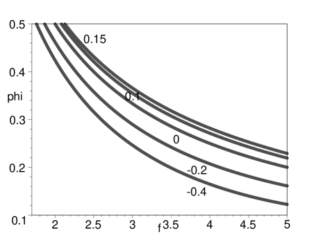
Figure 4: The evolution of the electric potential $\phi$ with respect to the physical radius ${f}$ for different $\alpha_{1}=-0.4,\ -0.2,\ 0,\,0.1,\ 0.15$. It shows that $\phi$ is regular in the spacetime except for $f=0$ (curvature singularity). The potential $\phi$ is divergent at the curvature singularity and asymptotically approaches zero in the infinity of space.

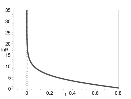
Figure 5: The evolution of the Ricci scalar $\ln R$ with respect to the physical radius ${f}$ with $m=1,\ \alpha_{0}=\alpha_{2}=1,\ \ \alpha=3/2,\ \ \ \alpha_{1}=-0.4$. It is apparent $R$ is divergent at $f=0$. This reveals that $f=0$ is indeed the curvature singularity of spacetime.

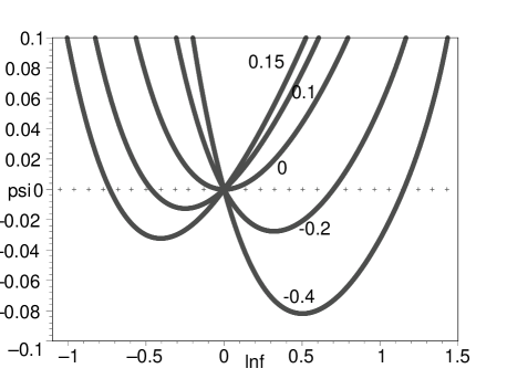
Figure 6: The evolution of the inverse of magnetic potential $\psi$ with respect to the physical radius $\ln{f}$ for different $\alpha_{1}=-0.4,\ -0.2,\ 0,\,0.1,\ 0.15$. It shows that the magnetic potential $\psi^{-1}$ is divergent on the inner Cauchy horizon and the outer black hole event horizon. On the curvature singularity and the spatial infinity, it asymptotically approaches zero.

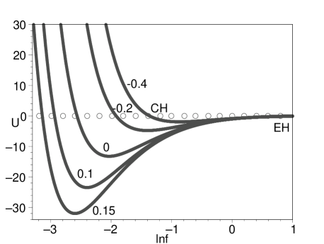
Figure 7: The evolution of $U$ with respect to the physical radius $\ln{f}$ with values $m=1,\ \alpha_{1}=\alpha_{2}=1,\ \ \alpha=3/2$. As for $\alpha_{0}$, we let $\alpha_{0}=0.15,\ 0.1,\ 0,\ -0.2,\ -0.4$, respectively. Comparing with Fig. 1, we find the black hole event horizon is pushed to infinity in this case. We are left with uniquely the inner Cauchy horizon. As an example, the CH and EH are given for $\alpha_{0}=-0.4$.

Finally, in order to understand the structure of horizons very well, it would be very helpful to investigate the trajectories of geodesic (free fall) paths in the spacetime. For simplicity, we shall restrict ourselves to timelike and radial geodesics. The equations of motion could be derived from the Lagrangian

$$\mathscr{L}=\frac{1}{2}\left[U\dot{t}^{2}-\frac{1}{U}\dot{r}^{2}-f^{2}\dot{r}^{2}-f^{2}\sin^{2}\theta\dot{\varphi}^{2}\right]\;,$$ (44)

where the dot denotes the differentiation with respect to the proper time $\tau$. They could also be derived from the geodesic equation

$$\frac{d^{2}X^{\mu}}{d\tau^{2}}+\Gamma^{\mu}_{\alpha\beta}\cdot\frac{dX^{\alpha}}{d\tau}\cdot\frac{dX^{\beta}}{d\tau}=0\;.$$ (45)

The equations of motion are found to be

$$\frac{dr}{d\tau}=-\sqrt{E^{2}-U}\;,$$ (46)

for proper time and

$$\frac{dr}{dt}=-\frac{U}{E}\cdot\sqrt{E^{2}-U}\;,$$ (47)

for coordinate time $t$, respectively. Here $E$ is a constant.

We shall consider the trajectories of particles which start from rest at some finite distance $r_{0}$ and fall towards the center. The constant $E$ is related to the starting distance $r_{0}$ by

$$E=\sqrt{U\mid_{r=r_{0}}}\;,\ \ (r=r_{0}\ \ \ \textrm{when}\ \ \dot{r}=0)$$ (48)

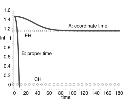
Figure 8: The evolution of coordinate time $t$ and proper time $\tau$ along a timelike radial geodesics of a test particle, starting at rest at $r_{0}=0.9\;$ or $\ln f_{0}=1.46$ and falling towards the singularity.

In Fig. 8, we plot the evolution of coordinate time $t$ and proper time $\tau$ along the timelike radial geodesics. The test particle starts at rest at $r_{0}=0.9\;$ or $\ln f_{0}=1.46$ and falls towards the singularity. The same as the Figures (1-6), the parameters are assumed with $f_{0}=1$, $m=1,\ \alpha_{0}=\alpha_{2}=1,\ \ \alpha=3/2$, $\alpha_{1}=-0.4$. The circled lines denote the black hole event horizon (EH) and the Cauchy horizon (CH), respectively(also shown in Fig. 1 and Fig. 3). Line A denotes the coordinate time $t$. It shows that with respect to an observer stationed at infinity, a particle describing a timelike trajectory will take an infinite time to reach the black hole event horizon. The behavior is in sharp contrast with that of proper time. Line B denotes the evolution of proper time $\tau$. It shows that the particle crosses the black hole event horizon and the Cauchy horizon with finite proper time. And after crossing the Cauchy horizon, the particle will arrive at some finite distance with finite proper time.

IV check of the solution with the Einstein equations

In section II, we construct the static spherically symmetric solution by imposing the symmetries of interest-rotational symmetry and statistic-on the action principle rather than on the field equations. Compared to the method of solving Einstein equations, it is relatively simple, but also seems questionable. The question is as follows. In imposing the symmetry before carrying the variation of the action principle, one generally loses field equations. So one may worry about that the solution maybe do not satisfy the lost equations contained in the Einstein equations. In this section, we shall check our solution with the Einstein equations. To this end, we should start from the total action of the theory which is given by

$$S=\int d^{4}x\sqrt{-g}\left[-{R}-\frac{c_{1}}{2}F_{\mu\nu}F^{\mu\nu}-c_{2}\left(\nabla_{\mu}A^{\mu}\right)^{2}+\lambda\left(A_{\mu}A^{\mu}+m^{2}\right)\right]\;.$$ (49)

In the first place, variation of the action with respect to $\lambda$, we obtain the equation of motion for $\lambda$

$$A_{\mu}A^{\mu}+m^{2}=0\;.$$ (50)

Actually, it is the fixed-norm constraint on the aether field.

Secondly, variation of the action with respect to $A^{\mu}$ leads to the equation of motion for aether field

$$c_{1}\nabla_{\nu}F^{\nu}_{\ \ \mu}+c_{2}\nabla_{\mu}\left(\nabla_{\nu}A^{\nu}\right)+\lambda A_{\mu}=0\;.$$ (51)

This equation determines the dynamics of $A^{\mu}$. Finally, variation of the action with respect to the metric gives the Einstein equations

$$G_{\mu\nu}=T_{\mu\nu}\;.$$ (52)

We emphasize that the equation of fixed-norm constraint Eq. (50) could be followed from the equation of motion of aether field Eq. (51) and the Einstein equations Eq. (52) in view of the fact that:

$$\nabla_{\nu}T^{\mu\nu}=0\;.$$ (53)

The energy-momentum tensor of the Einstein-aether field takes the form picon:09

$$T_{\mu\nu} = c_{1}F_{\mu\alpha}F_{\nu}^{\ \alpha}+c_{2}g_{\mu\nu}\left[A^{\alpha}\nabla_{\alpha}\left(\nabla_{\beta}A^{\beta}\right)+\left(\nabla_{\alpha}A^{\alpha}\right)^{2}\right]-2c_{2}A_{(\mu}\nabla_{\nu)}\left(\nabla_{\alpha}A^{\alpha}\right)$$ (54)

$$-\lambda A_{\mu}A_{\nu}+\frac{1}{2}g_{\mu\nu}\left[-\frac{c_{1}}{2}F_{\alpha\beta}F^{\alpha\beta}-c_{2}\left(\nabla_{\alpha}A^{\alpha}\right)^{2}-\lambda\left(A_{\alpha}A^{\alpha}+m^{2}\right)\right]\;.$$

Given the metric Eq. (3) and the aether field Eq. (4), we find the equation of motion for $\lambda$:

$$-\frac{1}{U}\phi^{2}+\frac{K^{2}}{Uf^{4}}+m^{2}=0\;,$$ (55)

the equation of motion for $A_{\mu}$:

$$c_{1}Uf\phi^{{}^{\prime\prime}}+2c_{1}U\phi^{{}^{\prime}}f^{{}^{\prime}}+\lambda\phi f=0\;,$$ (56)

$$c_{2}UfK^{{}^{\prime\prime}}-2c_{2}UK^{{}^{\prime}}f^{{}^{\prime}}+\lambda Kf=0\;.$$ (57)

and the Einstein equations:

$$\left(1-2Uff^{{}^{\prime\prime}}-U^{{}^{\prime}}ff^{{}^{\prime}}-Uf^{{}^{\prime}2}\right)\cdot\frac{1}{f^{2}} = \frac{1}{2}c_{1}\phi^{{}^{\prime}2}-\frac{1}{2}c_{2}K^{{}^{\prime}2}\frac{1}{f^{4}}+\lambda\left(\frac{K^{2}}{2Uf^{4}}-\frac{1}{2}m^{2}-\frac{1}{2}\frac{\phi^{2}}{U}\right)\;,$$ (58)

$$\left(1-Uf^{{}^{\prime}2}-U^{{}^{\prime}}ff^{{}^{\prime}}\right)\cdot\frac{1}{f^{2}} = \frac{1}{2}c_{1}\phi^{{}^{\prime}2}-\frac{1}{2}c_{2}K^{{}^{\prime}2}\frac{1}{f^{4}}+\lambda\left(-\frac{K^{2}}{2Uf^{4}}-\frac{1}{2}m^{2}+\frac{1}{2}\frac{\phi^{2}}{U}\right)\;,$$ (59)

$$-\frac{1}{2}U^{{}^{\prime\prime}}-Uf^{{}^{\prime\prime}}\frac{1}{f}-U^{{}^{\prime}}f^{{}^{\prime}}\frac{1}{f} = -\frac{1}{2}c_{1}\phi^{{}^{\prime}2}-\frac{1}{2}c_{2}K^{{}^{\prime}2}\frac{1}{f^{4}}-\lambda\left(-\frac{K^{2}}{2Uf^{4}}+\frac{1}{2}m^{2}-\frac{1}{2}\frac{\phi^{2}}{U}\right)\;,$$ (60)

which correspond to $G_{0}^{0}=T_{0}^{0}$, $G_{1}^{1}=T_{1}^{1}$ and $G_{2}^{2}=T_{2}^{2}$ , respectively. Now we have six equations of motion but five variables, namely, $U,\ f,\ \phi,\ K,\ \lambda$. Therefore, among the six equations, only five of them are independent. It is indeed the case when we take into account the fact that the equation of motion for $\lambda$ Eq. (50) follows from the equation of motion of aether field Eq. (51) and the Einstein equations Eq. (52). In practice, one could show that Eq. (55) follows from Eqs.(56-60) by using of Eq. (53).

One may ask whether the five equations of motion Eqs. (9-13) derived with the Euler-Lagrange method could be derived from above six equations of motion Eqs. (55-66). The answer is yes. In fact, we have

$$\textrm{Eq.}\left(9\right)\Longleftrightarrow\textrm{Eq.}\left(55\right)\;,$$

$$\textrm{Eq.}\left(10\right)\Longleftrightarrow\textrm{Eq.}\left(56\right)\;,$$

$$\textrm{Eq.}\left(11\right)\Longleftrightarrow\textrm{Eq.}\left(57\right)\;,$$

$$\textrm{Eq.}\left(12\right)\Longleftrightarrow\textrm{Eq.}\left(58\right)-\textrm{Eq.}\left(59\right)\;,$$

$$\textrm{Eq.}\left(13\right)\Longleftrightarrow\textrm{Eq.}\left(60\right)\;.$$

Now we could understand that our solution satisfies all the equations: the fixed-norm constraint equation, the equation of motion of $A_{\mu}$ and the Einstein equations.

V conclusion and discussion

In conclusion, a static spherically symmetric solution in the Einstein-aether is obtained. Due to the complication of the Einstein equations, we prefer to deal with the Euler-Lagrange equations. This method is relatively simple and the same as the Einstein equations in nature. By this way, an exact solution is constructed. The solution is similar to the Reissner-Nordstrom solution in that it has an inner Cauchy horizon and an outer black hole event horizon. But a remarkable difference from the Reissner-Nordstrom solution is that it is not asymptotically flat in space. We find the solution asymptotically approaches a two dimensional sphere. The resulting electric potential is regular in the whole spacetime except for the curvature singularity. On the other hand, the magnetic potential is divergent on both Cauchy horizon and the outer event horizon.

References

(1) T. Jacobson and D. Mattingly,
Phys. Rev. D 64, 024028 (2001). [arXiv:grqc/ 0007031].
(2) T. Jacobson, PoS QG-PH, 020 (2007) [arXiv:0801.1547].
(3) E. A. Lim, Phys. Rev. D 71, 063504 (2005) [arXiv:astro-ph/0407437].
(4) M. Nakashima and T. Kobayashi, [arXiv:astro-ph/1012.5348].
(5)S. M. Carroll, T. R. Dulaney, M. I. Gresham, H. T. Phys. Rev.D79: 065011 (2009);
(6)S. M. Carroll, T. R. Dulaney, M. I. Gresham,
H. T. Phys. Rev.D79: 065012 (2009);
(7)S. M. Caroll, et
al, Phys. Rev. D 79, 065011 (2009);
(8)C. Armendariz-Picon, N. F. Sierra and
J. Garriga, JCAP. 07, 010 (2010);
(9) S. M. Carroll and E. A. Lim, Phys. Rev. D 70, 123525 (2004)
[arXiv:hep-th/0407149].
(10)C. Bonvin, R. Durrer, et al, Phys. Rev. D 77, 024037 (2008)
(11)J. D. Barrow, Phys. Rev. D 85, 047503 (2012)
(12)D. Garfinkle, C. Eling, T. Jacobson, Phys. Rev.
D76, 024003 (2007). [gr-qc/0703093].
(13)T. Jacobson and D. Mattingly, Phys.
Rev. D 70, 024003 (2004) [arXiv:gr-qc/0402005];
(14)B. Z. Foster, Phys. Rev. D 73,
104012 (2006) [arXiv:gr-qc/0602004].
(15) C. Eling and T. Jacobson, Class. Quant. Grav. 23, 5643 (2006) [arXiv:gr-
qc/0604088].