The unifying theory of scaling in thermal convection: The updated prefactors
Abstract
The unifying theory of scaling in thermal convection (Grossmann & Lohse (2000)) (henceforth the GL theory) suggests that there are no pure power laws for the Nusselt and Reynolds numbers as function of the Rayleigh and Prandtl numbers in the experimentally accessible parameter regime. In Grossmann & Lohse (2001) the dimensionless parameters of the theory were fitted to 155 experimental data points by Ahlers & Xu (2001) in the regime and and Grossmann & Lohse (2002) used the experimental data point from Qiu & Tong (2001) and the fact that is independent of the parameter , which relates the dimensionless kinetic boundary thickness with the square root of the wind Reynolds number, to fix the Reynolds number dependence. Meanwhile the theory is on one hand well confirmed through various new experiments and numerical simulations. On the other hand these new data points provide the basis for an updated fit in a much larger parameter space. Here we pick four well established (and sufficiently distant) Nu(Ra,Pr) data points and show that the resulting function is in agreement with almost all established experimental and numerical data up to the ultimate regime of thermal convection, whose onset also follows from the theory. One extra data point is used to fix . As can depend on the definition and the aspect ratio the transformation properties of the GL equations are discussed in order to show how the GL coefficients can easily be adapted to new Reynolds number data while keeping unchanged.
1 Introduction
Thermal convection is omnipresent in science and technology and its paradigmatical representation is Rayleigh-Bénard (RB) convection: a fluid in a sample heated from below and cooled from above. This system has received considerable attention in the last decades (Ahlers et al., 2009b; Siggia, 1994; Lohse & Xia, 2010), with one focus on the scaling properties of the global heat transport of the system. The now widely accepted viewpoint is the Grossmann-Lohse (GL) theory (Grossmann & Lohse, 2000, 2001, 2002, 2004). The basis for this theory of scaling in RB convection are exact global balances for the energy and thermal dissipation rates derived from the Boussinesq equations and the decomposition of the flow in boundary layer (BL) and bulk contributions. The scaling of the dissipation rates in the BLs is assumed to obey Prandtl-Blasius-Pohlhausen scaling (Schlichting, 1979), which is justified as long as the shear-Reynolds numbers of the BLs are not too large, and the scaling relations in the bulk are estimated based on Kolmogorov-type arguments for homogeneous isotropic turbulence. While the theory gives the different scaling relations for the individual contributions to the energy dissipation rates in the bulk and in the BL, namely and , and to the thermal dissipation rates in the bulk (background) and in the BLs (plus the plumes, see Grossmann & Lohse (2004)), namely and , the absolute sizes of these four relative contributions are not given by the theory. They are expressed in four dimensionless prefactors , for , , , and , respectively, which have to be obtained from experimental or numerical data for .
When the theory was developed early this century, such data were scarce and often contradicting each other, due to sidewall and plate effects, insufficient knowledge of the material properties of the fluid, lack of numerical resolution and other problems. Grossmann & Lohse (2001) used 155 data points for in the parameter range and obtained by Ahlers & Xu (2001), which was the most extensive data set at that time. This fixed for all and , considered as valid up to the meanwhile found (He et al. (2012b)) ultimate regime of thermal convection, where the Prandtl-Blasius type BL becomes unstable. was fixed (cf. Grossmann & Lohse (2002)) with one extra adoption of the prefactor , i.e. the amplitude parameter of the Prandtl BL thickness, in the Prandtl-Blasius scaling relation , to the experimental data of Qiu & Tong (2001), where is the mean thickness of the kinetic BL and the height of the sample.
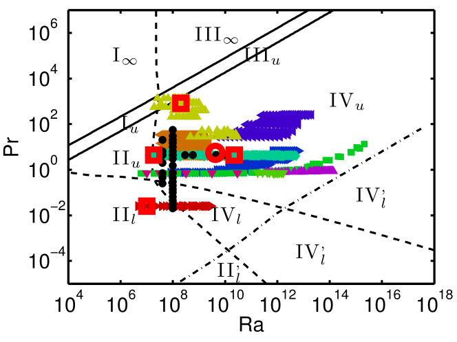

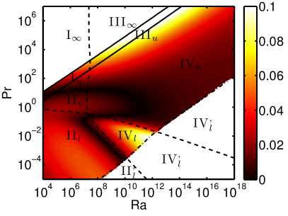
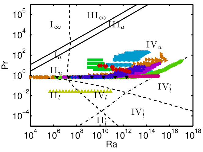
Although the data to which we adopted the four prefactors and were relatively local in parameter space, the theory was rather successful in describing the global behavior and also , as described in detail in Ahlers et al. (2009b). This included the prediction that for the onset to the ultimate regime should take place when Ra is of the order of . This prediction was based on an assumed onset of a sheared BL instability at a shear Reynolds number , which is the value given in Landau & Lifshitz (1987). Indeed, very recently He et al. (2012b) have found the onset of the ultimate regime at this very Rayleigh number. Thanks to joint efforts of the community the experimental and numerical data situation for has considerably improved in the last decade. Measurements have been extended to a much larger domain in the Ra-Pr parameter space, see the updated phase diagrams in figure 1 and figure 8, and plate- and sidewall corrections are much better understood and taken into account (Brown et al. (2005); Ahlers (2000); Roche et al. (2001); Verzicco (2002); Niemela & Sreenivasan (2003); Ahlers et al. (2009b)). One notices that for higher Ra number values have been obtained than for , while the number dependence is much more explored for than for . Furthermore, due to the increasing computational power and better codes the numerical data are now well converged, confirming and complementing the experimental data. Meanwhile Stevens et al. (2010c, 2011a) achieved at in a sample and obtained a good agreement with the experimental data of He et al. (2012b) and Niemela et al. (2000).
This situation calls for a refit of the four prefactors and of the GL theory, in spite of the success of the theory with the coefficients of Grossmann & Lohse (2001): It is clear that the surface above the Ra-Pr parameter space will be much more stable and ”wobble” less if we put it on four distant and trustable ”legs” , , rather than putting it on four ”legs” somewhere in the center but close to each other. As we will see is only determined by the choice of these four data points from experiments. The accuracy of the GL-fit is verified by comparing it with several data sets over a wide parameter regime and by making a second fit that reveals in which regimes there is some uncertainty. Including more data points in the fitting procedure does not lead to better fits since data tend to be clustered in the phase space. Therefore including more data points increases the weight of some data without actually adding additional physical information. An additional Reynolds number measurement is necessary to fix and the relation between and , which is the Reynolds number for which no bulk is left and the whole flow consists of laminar boundary layer as will be explained below. The shortcoming of the old set of , , and was particularly obvious for small , say (see figure 5), because at the days of Grossmann & Lohse (2001) no reliable information was available in that parameter regime and therefore no Nusselt data of that regime had been included into the fit.
The structure of the paper is as follows: In section 2 we will provide the refit of the GL theory for an aspect ratio , leading to in the whole parameter space up to the ultimate state. In section 3 we discuss the robustness of the fit. In section 4 we will show that this fit also describes the available data for and will in particular discuss the onset of the ultimate regime. Section 5 gives conclusions and an outlook on the new challenges.
2 Refit of the GL theory for
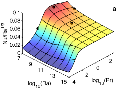
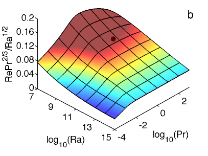
The GL theory describes Nu(Ra,Pr) and Re(Ra,Pr) with the following two coupled equations (Ahlers et al. (2009b)),
| (1) | |||||
| (2) | |||||
where the crossover functions f and g model the crossover from the thermal boundary layer nested in the kinetic one towards the inverse situation and that for which looses its scaling with Re since extends to sample half-height and cannot increase further with decreasing Re; for details see Grossmann & Lohse (2001). As described by Grossmann & Lohse (2002) the prefactor has to be determined from experimental data. Whereas the definition of the Nusselt number is very clear there are various reasonable ways to define a Reynolds number. We decided to use one experimental data point of Qiu & Tong (2001) to determine the value of and from figure 1 of Grossmann & Lohse (2002) we read Ra=4.2, Pr=5.5, Re=2.1 . In addition we demand for the Reynolds number that , meaning that is fixed for given .
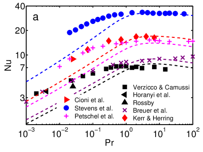
In order to get accurate values for the four dimensionless prefactors , it is necessary to choose four data points with as much information on the richness of the RB system as possible, which means that data points from different regimes should be selected. Therefore we determined the from the data points of Funfschilling et al. (2005) at and , both with , the data point from Xia et al. (2002) with at , and the data point from Cioni et al. (1997) at with . The location of these data points in the RB phase diagram is indicated by the large red squares in figure 1 and by the black dots in the corresponding three-dimensional Nu(Ra,Pr) visualization in figure 2a. Figure 1 shows that these data are indeed within different regimes. The reason for choosing these specific data points is two-fold. First of all we consider these four data points to be reliable. And apart from the data point by Xia et al. (2002), which is the only experiment in that large regime, all data points agree very well with experimental or numerical data from other groups, see figures 3 and 5. In addition, these four data points are relatively far apart in the Ra-Pr parameter space to ensure that they provide the theory with as much information on the richness of the RB physics as possible. To provide information on the -scaling we selected the measurements of Funfschilling et al. (2005) at and with . In order to include information on the transition between the ’upper’ and ’lower’ regimes, which is modeled by the crossover functions and , it is necessary to include data points in the low, intermediate, and high Pr number regime. We do this selecting next to the intermediate Pr number data from Funfschilling et al. (2005), the low number measurement by Cioni et al. (1997) at and the high measurement by Xia et al. (2002) at . Altogether the four data points provide information from three different Pr numbers and four different Ra numbers. From these four data points, and an initial guess for , we determine the with a fourth order Newton-Raphson root finding method or by using a trust-region-reflective optimization algorithm, which both gave the same result. Subsequently, the point of Qiu & Tong (2001) is used to find the appropriate value of with the transformation property of the GL model (Grossmann & Lohse (2002)), which is described below in detail. Due to this transformation property of the GL equations the four data points determine the Nusselt number dependence, while the Re number data point of Qiu & Tong (2001) fixes the absolute value of the Reynolds number throughout the phase space. This results in the following five GL parameters , , , , and . The difference in significant number is due to the fact that some coefficients are less sensitive to uncertainty than others.
It was pointed out by Grossmann & Lohse (2002) that is invariant and thus independent of the parameter under the following transformation
| (3) | |||||
| (4) | |||||
| (5) | |||||
| (6) | |||||
| (7) | |||||
| (8) | |||||
| (9) |
We note that the above transformation is consistent with the relation used above and allows for the transformation of the above set of coefficients to different Reynolds number definitions or aspect ratios. Such a new set of coefficients is obtained by first determining . Here is determined as , where is the Reynolds number value of a measurement point in the data set at a given and and is the Reynolds number value obtained from the GL model with the coefficients mentioned above. Subsequently, equations (4) to (9) can be used to calculate the new coefficients.
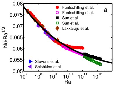
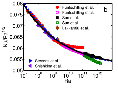
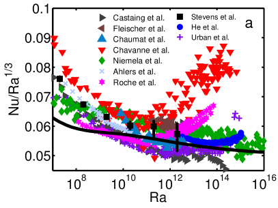
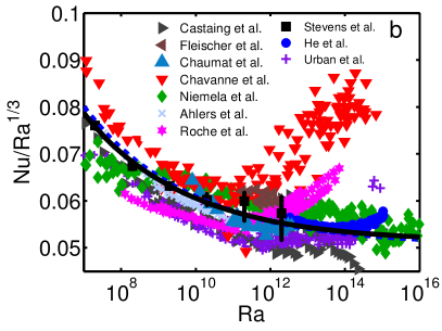
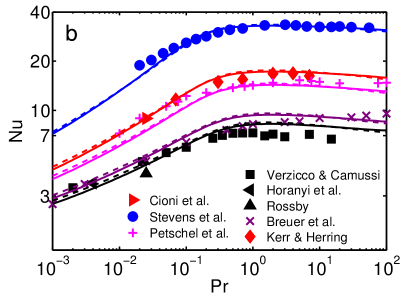
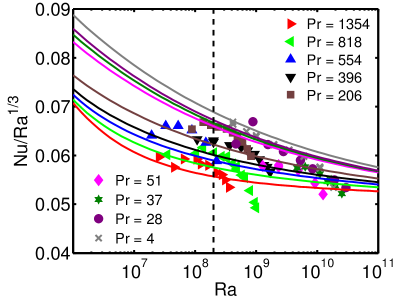
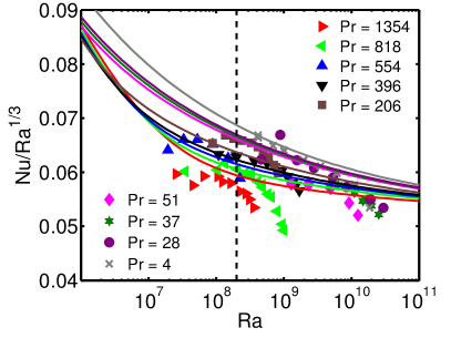
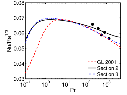
In figures 3 to 5 we compare the original GL-fit from Grossmann & Lohse (2001) with this new GL-fit. These figures clearly reveal that the new GL-fit is much closer to the data in the low number regime, while maintaining the similar excellent agreement for the high number data as before. We emphasize that this excellent agreement with all other presently available data from experiments and simulations confirms that the and values we calculated describes well in the regime that is nowadays covered by state of the art experiments and simulations. It is also noteworthy that figure 3 and 4 show that the number scaling with is well predicted by the GL-theory for values that are decades higher than the highest number point that is used to determine the values, namely , thus showing the predictive power of the GL-theory.
3 Robustness
To illustrate the robustness of the fit presented above, we made a second fit to four other data points, i.e. the data points from Funfschilling et al. (2005) at and with , the one from Xia et al. (2002) at with and finally the data point by Kerr & Herring (2000) at with . Three out of these four data points lie relatively close to the original four data points, but the low point from Kerr & Herring (2000) substantially differs from the original . The reason that three of the four points are close to the original four points in the parameter space is that one can only select ”reliable legs” in regimes were many measurements have been done and these regimes only cover a limited part of the parameter space.
The resulting GL coefficients are , , , , and compared to , , , , and of the fit described above. In order to compare the two fits we show both fits together with experimental and numerical data from several experiments in figures 3, 4, 5, and 7. In addition we give the relative difference in calculated in the fit described in the previous section and calculated from this additional fit in the parts of the parameter space where the GL fit is valid in figure 6. A comparison between both fits shows that the difference is very minor in the regimes , , and , and that the differences increase in the regimes , , and , which are very far away from the region in the parameter space where reliable data points are available. The reason is that a very small variation in the measurements point can lead to significant differences if the implied information is extrapolated over many decades in and using the GL-theory. For the fits compared here the differences increase up to about . We find that the differences are mainly caused by the uncertainty in the Xia et al. (2002) data, which is reflected by the two different data points we took from this data set. In figure 7 we compare the Xia et al. (2002) measurements with the original GL-fit from Grossmann & Lohse (2001), and the two fits presented in this work. Panels a, b and c show that the measured decreases faster with increasing Ra than predicted by the GL model. A comparison of the Xia et al. (2002) data with other data obtained at shows that the measurements in the lower number regime collapse very well with other measurements, while for the higher the measured Nusselt number seems a little lower in the Xia et al. (2002) experiments than in other experiments. Figure 7d compares the Xia et al. (2002) measurements between and with the different GL-fits and shows that the fit presented in section 2 uses a high Pr number point that aligns with the reliable data point, while the second fit uses a high number point of the lower branch. In this way the uncertainty of these measurements is reflected by the two fits and as is shown in figure 6 this difference is mostly visible near regime and .

4 GL theory for and ultimate regime
In principle, the depend on the aspect ratio . However, it is well known that only small differences in are observed between and (Ahlers et al. (2009b)). This weak aspect ratio dependence is confirmed by figure 4, which shows that the number scaling for in a sample is captured very accurately by the new fit for , and in the low Ra number regime the new fit is even much better than the original GL-fit from Grossmann & Lohse (2001).
The location in Ra-Pr space of the various regimes of the GL theory is based on the coefficients and . The updated lines that encompass the regimes are plotted in the phase diagrams shown in figures 1 and 8. The line that indicates the onset of the ultimate regime, where the kinetic boundary layer has become turbulent, is now based on the new coefficients, the transition at , observed by He et al. (2012b) for , and the number measurements by Qiu & Tong (2001). This gives () and for the second fit we made, see section 3, we get (). In a sample He et al. (2012b) found experimentally that using a recently developed and tested elliptic approximation (He & Zhang (2006); Zhao & He (2009); He et al. (2010); He & Tong (2011); Zhou et al. (2011)), which defines unambiguously, based on properties of correlation functions. Using this relation at and this gives with for the first fit, see section 2, and with for the second fit we made, see section 3. These values are different from the previously used with taken from pipe flow (Landau & Lifshitz (1987)). From the transformation property of the GL equations one gets that increases by a factor of when increases by a factor , while increases by a factor . The values found here are significantly different from , which was found by Grossmann & Lohse (2002). Calculating the values equivalent to from the and combinations mentioned above, i.e. with , with , with , and with , gives for the new coefficients, so we see that the notification of alone, without is not sufficient.
The phase diagram in figure 8 shows that the measurements of He et al. (2012b) up to at are up to now the only experiments that have reached the ultimate regime. They observe the onset of the ultimate regime at and a transition region for . The experiments by He et al. (2012b) are the only room temperature experiments for , while all other experiments that have reached these Ra numbers are low temperature experiments with Helium close to the critical point (Chavanne et al. (1997, 2001); Niemela et al. (2000, 2001); Niemela & Sreenivasan (2006); Roche et al. (2010); Urban et al. (2011, 2012)). In these low temperature experiments it is difficult to reach the ultimate regime because the Pr number increases with increasing Ra, see figure 8. Nevertheless the low temperature experiments by Niemela et al. (2000) seem to come very close to the ultimate regime and one may wonder why the transition region observed by He et al. (2012b) was not observed in the Niemela et al. (2000) experiments. As discussed in detail by Ahlers et al. (2012b), presumably the scatter of the Niemela et al. (2000) data at this highest Ra (which seems to be due primarily to the uncertainties in the fluid properties) as well as the fact that the transition is smooth are the reasons for this. Figure 4 shows that the magnitude of the scatter in the Niemela et al. (2000) data is similar to the observed increase in the compensated Nusselt number in the transition regime by He et al. (2012b). The phase diagram also shows that other low temperature experiments by Chavanne et al. (1997, 2001), Roche et al. (2010), and Urban et al. (2011, 2012) do not reach the ultimate regime and therefore no transition to the ultimate regime due to a boundary layer shear instability is expected in these experiments.

5 Conclusions and outlook
In this paper we have used the availability of new experimental and numerical data, and our increased understanding of the physics of the Rayleigh-Bénard system to determine the prefactors of the unifying theory for scaling in thermal convection, i.e. the GL theory, much more accurately. The resulting function is in very good agreement with almost all established experimental and numerical data up to the ultimate regime of thermal convection, and has significantly improved the predictions. In figure 4 one can notice the onset of the ultimate regime in the Nu(Ra) scaling of the measurements of He et al. (2012b). Extensions of the GL theory to the ultimate regime by Grossmann & Lohse (2011) are able to explain the observed Reynolds number scaling in that regime as well as the origin of the log-profiles observed in the ultimate regime by Ahlers et al. (2012a).
In line with Grossmann & Lohse (2001), we have determined the prefactors from experimental measurements. This has great value as it shows that the information of only five data-points is sufficient to accurately predict and up to the ultimate regime. All is based on the GL theory, which builds on exact global balances for the energy and thermal dissipation rates, derived from the Boussinesq equations, and the decomposition of the flow in boundary layer and bulk contributions. A finding with further implications is that the value , i.e. the amplitude parameter of the Prandtl BL thickness, is higher than found by Grossmann & Lohse (2002). This value is for example used by Shishkina et al. (2010) to determine the number of grid points that should be placed in the boundary layers. Shishkina et al. (2010) compared the theoretical predictions with results from simulations in samples. For this aspect ratio the newly found value of a ( for fit of section 2 and of section 3) is higher, but still relatively close to the previously used . However, it looks like that for case is even higher ( for the fit of section 2 and for the fit of section 3), which could have implications for the resolution that should be used in simulations. This finding confirms the conclusions of Stevens et al. (2010c) who pointed out that the only way to really confirm that the used numerical resolution is sufficient is to obtain the same Nusselt number with different grids resolutions as there is namely always some uncertainty in estimates of the required grid resolution.
A further challenge we want to pursue is to calculate the and directly from the fluid equations, without the input of any experimental or numerical data, or at least quantitatively relate their values to important fluid concepts like Prandtl-Blasius-Pohlhausen theory, the von Karman-Prandtl theory, etc. in order to get an even deeper understanding of the GL theory.
Acknowledgments
We thank all of our colleagues for various discussions over the years and G. Ahlers, F. Chilla, K. Petschel, P. Roche, L. Skrbek, R. Verzicco, and K.-Q. Xia for providing us with their experimental and numerical data and for numerous scientific discussions and insightful remarks on RB over the years. Special thanks goes to G. Ahlers for his insightful comments on earlier versions of this manuscript. We acknowledge the Foundation for Fundamental Research of Matter (FOM), which is part of NWO, for funding.
References
- Ahlers (2000) Ahlers, G. 2000 Effect of sidewall conductance on heat-transport measurements for turbulent Rayleigh-Bénard convection. Phys. Rev. E 63, 015303–1 – 4.
- Ahlers et al. (2012a) Ahlers, G., Bodenschatz, E., Funfschilling, D., Grossmann, S., He, X., Lohse, D., Stevens, R.J.A.M. & Verzicco, R. 2012a Logarithmic temperature profiles in turbulent Rayleigh-Bénard convection. Phys. Rev. Lett. 109, 114501.
- Ahlers et al. (2009a) Ahlers, G., Bodenschatz, E., Funfschilling, D. & Hogg, J. 2009a Turbulent Rayleigh-Bénard convection for a Prandtl number of 0.67. J. Fluid. Mech. 641, 157–167.
- Ahlers et al. (2009b) Ahlers, G., Grossmann, S. & Lohse, D. 2009b Heat transfer and large scale dynamics in turbulent Rayleigh-Bénard convection. Rev. Mod. Phys. 81, 503.
- Ahlers et al. (2012b) Ahlers, G., He, X., Funfschilling, D. & Bodenschatz, E. 2012b Heat transport by turbulent Rayleigh-Bénard convection for Pr=0.8 and : aspect ratio =0.50. New J. Phys. 14, 063030.
- Ahlers & Xu (2001) Ahlers, G. & Xu, X. 2001 Prandtl-number dependence of heat transport in turbulent Rayleigh-Bénard convection. Phys. Rev. Lett. 86, 3320–3323.
- Breuer et al. (2004) Breuer, M., Wessling, S., Schmalzl, J. & Hansen, U. 2004 Effect of inertia in Rayleigh-Bénard convection. Phys. Rev. E 69, 026302.
- Brown et al. (2005) Brown, E., Funfschilling, D., Nikolaenko, A. & Ahlers, G. 2005 Heat transport by turbulent Rayleigh-Bénard convection: Effect of finite top- and bottom conductivity. Phys. Fluids 17, 075108.
- Burnishev et al. (2010) Burnishev, Y., Segre, E. & Steinberg, V. 2010 Strong symmetrical non-Oberbeck Boussinesq turbulent convection and the role of compressibility. Phys. Fluids 22, 035108.
- Castaing et al. (1989) Castaing, B., Gunaratne, G., Heslot, F., Kadanoff, L., Libchaber, A., Thomae, S., Wu, X. Z., Zaleski, S. & Zanetti, G. 1989 Scaling of hard thermal turbulence in Rayleigh-Bénard convection. J. Fluid Mech. 204, 1–30.
- Chaumat et al. (2002) Chaumat, S., Castaing, B. & Chilla, F. 2002 Rayleigh-Bénard cells: influence of plate properties. In Advances in Turbulence IX (ed. I. P. Castro, P. E. Hancock & T. G. Thomas). Barcelona: International Center for Numerical Methods in Engineering, CIMNE.
- Chavanne et al. (1997) Chavanne, X., Chilla, F., Castaing, B., Hebral, B., Chabaud, B. & Chaussy, J. 1997 Observation of the ultimate regime in Rayleigh-Bénard convection. Phys. Rev. Lett. 79, 3648–3651.
- Chavanne et al. (2001) Chavanne, X., Chilla, F., Chabaud, B., Castaing, B. & Hebral, B. 2001 Turbulent Rayleigh-Bénard convection in gaseous and liquid he. Phys. Fluids 13, 1300–1320.
- Cioni et al. (1997) Cioni, S., Ciliberto, S. & Sommeria, J. 1997 Strongly turbulent Rayleigh-Bénard convection in mercury: comparison with results at moderate Prandtl number. J. Fluid Mech. 335, 111–140.
- Emran & Schumacher (2012) Emran, M. S. & Schumacher, J. 2012 Conditional statistics of thermal dissipation rate in turbulent Rayleigh-Bénard convection. Eur. Phys. J. E 108, 35.
- Fleischer & Goldstein (2002) Fleischer, A. S. & Goldstein, R. J. 2002 High-Rayleigh-number convection of pressurized gases in a horizontal enclosure. J. Fluid Mech. 469, 1–12.
- Funfschilling et al. (2005) Funfschilling, D., Brown, E., Nikolaenko, A. & Ahlers, G. 2005 Heat transport by turbulent Rayleigh-Bénard convection in cylindrical cells with aspect ratio one and larger. J. Fluid Mech. 536, 145–154.
- Glazier et al. (1999) Glazier, J. A., Segawa, T., Naert, A. & Sano, M. 1999 Evidence against ultrahard thermal turbulence at very high Rayleigh numbers. Nature 398, 307–310.
- Grossmann & Lohse (2000) Grossmann, S. & Lohse, D. 2000 Scaling in thermal convection: A unifying view. J. Fluid. Mech. 407, 27–56.
- Grossmann & Lohse (2001) Grossmann, S. & Lohse, D. 2001 Thermal convection for large Prandtl number. Phys. Rev. Lett. 86, 3316–3319.
- Grossmann & Lohse (2002) Grossmann, S. & Lohse, D. 2002 Prandtl and Rayleigh number dependence of the Reynolds number in turbulent thermal convection. Phys. Rev. E 66, 016305.
- Grossmann & Lohse (2004) Grossmann, S. & Lohse, D. 2004 Fluctuations in turbulent Rayleigh-Bénard convection: The role of plumes. Phys. Fluids 16, 4462–4472.
- Grossmann & Lohse (2011) Grossmann, S. & Lohse, D. 2011 Multiple scaling in the ultimate regime of thermal convection. Phys. Fluids 23, 045108.
- He & Zhang (2006) He, G. W. & Zhang, J. B. 2006 Elliptic model for space-time correlations in turbulent shear flows. Phys. Rev. E 73, 055303.
- He et al. (2012a) He, X., Funfschilling, D., Bodenschatz, E. & Ahlers, G. 2012a Heat transport by turbulent Rayleigh-Bénard convection for Pr=0.8 and for aspect ratio =1.00. New J. Phys. 14, 103012.
- He et al. (2012b) He, X., Funfschilling, D., Nobach, H., Bodenschatz, E. & Ahlers, G. 2012b Transition to the ultimate state of turbulent Rayleigh-Bénard convection. Phys. Rev. Lett. 108, 024502.
- He et al. (2010) He, X., He, G. & Tong, P. 2010 Small-scale turbulent fluctuations beyond Taylor s frozen-flow hypothesis. Phys. Rev. E 81, 065303.
- He & Tong (2011) He, X. & Tong, P. 2011 Kraichnan s random sweeping hypothesis in homogeneous turbulent convection. Phys. Rev. E 83, 037302.
- Horanyi et al. (1999) Horanyi, S., Krebs, L. & Müller, U. 1999 Turbulent Rayleigh-Bénard convection in low prandtl number fluids. Int. J. Heat Mass Transfer 42, 3983–4003.
- Kerr & Herring (2000) Kerr, R. & Herring, J. R. 2000 Prandtl number dependence of nusselt number in direct numerical simulations. J. Fluid Mech. 419, 325–344.
- Lakkaraju et al. (2012) Lakkaraju, R., Stevens, R.J.A.M., Verzicco, R., Grossmann, S., Prosperetti, A., Sun, C. & Lohse, D. 2012 Spatial distribution of heat flux and fluctuations in turbulent Rayleigh-Bénard convection. Phys. Rev. E 86, 056315.
- Landau & Lifshitz (1987) Landau, L. D. & Lifshitz, E. M. 1987 Fluid Mechanics. Oxford: Pergamon Press.
- Lohse & Xia (2010) Lohse, D. & Xia, K. Q. 2010 Small-scale properties of turbulent Rayleigh-Bénard convection. Annu. Rev. Fluid Mech. 42, 335–364.
- Niemela et al. (2000) Niemela, J., Skrbek, L., Sreenivasan, K. R. & Donnelly, R. 2000 Turbulent convection at very high Rayleigh numbers. Nature 404, 837–840.
- Niemela et al. (2001) Niemela, J., Skrbek, L., Sreenivasan, K. R. & Donnelly, R. J. 2001 The wind in confined thermal turbulence. J. Fluid Mech. 449, 169–178.
- Niemela & Sreenivasan (2003) Niemela, J. & Sreenivasan, K. R. 2003 Confined turbulent convection. J. Fluid Mech. 481, 355–384.
- Niemela & Sreenivasan (2006) Niemela, J. & Sreenivasan, K. R. 2006 Turbulent convection at high Rayleigh numbers and aspect ratio 4. J. Fluid Mech. 557, 411 – 422.
- Petschel et al. (2013) Petschel, K., Stellmach, S., Wilczek, M., Lülff, J. & Hansen, U. 2013 Dissipation layers in Rayleigh-Bénard convection: A unifying view. to appear in Phys. Rev. Lett., see also arXiv:1212.5073 .
- van der Poel et al. (2013) van der Poel, E. P., Stevens, R.J.A.M. & Lohse, D. 2013 Comparison between two and three dimensional Rayleigh-Bénard convection. Submitted to J. Fluid Mech. .
- Qiu & Tong (2001) Qiu, X. L. & Tong, P. 2001 Large scale velocity structures in turbulent thermal convection. Phys. Rev. E 64, 036304.
- Roche et al. (2001) Roche, P.E., Castaing, B., Chabaud, B., Hebral, B. & Sommeria, J. 2001 Side wall effects in Rayleigh-Bénard experiments. Eur. Phys. J. B 24, 405–408.
- Roche et al. (2010) Roche, P.-E., Gauthier, F., Kaiser, R. & Salort, J. 2010 On the triggering of the ultimate regime of convection. New J. Phys. 12, 085014.
- Rossby (1969) Rossby, H. T. 1969 A study of Bénard convection with and without rotation. J. Fluid Mech. 36, 309–335.
- Schlichting (1979) Schlichting, H. 1979 Boundary layer theory, 7th edn. New York: McGraw Hill book company.
- Shishkina et al. (2010) Shishkina, O., Stevens, R. J. A. M., Grossmann, S. & Lohse, D. 2010 Boundary layer structure in turbulent thermal convection and its consequences for the required numerical resolution. New J. Phys. 12, 075022.
- Shishkina & Thess (2009) Shishkina, O. & Thess, A. 2009 Mean temperature profiles in turbulent Rayleigh–Bénard convection of water. J. Fluid Mech. 633, 449–460.
- Siggia (1994) Siggia, E. D. 1994 High Rayleigh number convection. Annu. Rev. Fluid Mech. 26, 137–168.
- Stevens et al. (2010a) Stevens, R. J. A. M., Clercx, H. J. H. & Lohse, D. 2010a Boundary layers in rotating weakly turbulent Rayleigh-Bénard convection. Phys. Fluids 22, 085103.
- Stevens et al. (2010b) Stevens, R. J. A. M., Clercx, H. J. H. & Lohse, D. 2010b Optimal Prandtl number for heat transfer in rotating Rayleigh-Bénard convection. New J. Phys. 12, 075005.
- Stevens et al. (2011a) Stevens, R. J. A. M., Lohse, D. & Verzicco, R. 2011a Prandtl number dependence of heat transport in high Rayleigh number thermal convection. J. Fluid. Mech. 688, 31–43.
- Stevens et al. (2011b) Stevens, R. J. A. M., Overkamp, J., Lohse, D. & Clercx, H. J. H. 2011b Effect of aspect-ratio on vortex distribution and heat transfer in rotating Rayleigh-Bénard convection. Phys. Rev. E 84, 056313.
- Stevens et al. (2010c) Stevens, R. J. A. M., Verzicco, R. & Lohse, D. 2010c Radial boundary layer structure and Nusselt number in Rayleigh-Bénard convection. J. Fluid. Mech. 643, 495–507.
- Sun et al. (2005) Sun, C., Ren, L.-Y., Song, H. & Xia, K.-Q. 2005 Heat transport by turbulent Rayleigh-Bénard convection in 1m diameter cylindrical cells of widely varying aspect ratio. J. Fluid Mech. 542, 165–174.
- Sun & Xia (2005) Sun, C. & Xia, K.-Q. 2005 Scaling of the Reynolds number in turbulent thermal convection. Phys. Rev. E 72, 067302.
- Urban et al. (2012) Urban, P., Hanzelka, P., Kralik, T., Musilova, V., Srnka, A. & Skrbek, L. 2012 Effect of boundary layers asymmetry on heat transfer efficiency in turbulent Rayleigh-Bénard convection at very high Rayleigh numbers. Phys. Rev. Lett. 109, 154301.
- Urban et al. (2011) Urban, P., Musilová, V. & Skrbek, L. 2011 Efficiency of heat transfer in turbulent Rayleigh-Bénard convection. Phys. Rev. Lett. 107, 014302.
- Verzicco (2002) Verzicco, R. 2002 Sidewall finite conductivity effects in confined turbulent thermal convection. J. Fluid Mech. 473, 201–210.
- Verzicco & Camussi (1999) Verzicco, R. & Camussi, R. 1999 Prandtl number effects in convective turbulence. J. Fluid Mech. 383, 55–73.
- Xia et al. (2002) Xia, K.-Q., Lam, S. & Zhou, S. Q. 2002 Heat-flux measurement in high-Prandtl-number turbulent Rayleigh-Bénard convection. Phys. Rev. Lett. 88, 064501.
- Zhao & He (2009) Zhao, X. & He, G.-W. 2009 Space-time correlations of fluctuating velocities in turbulent shear flows. Phys. Rev. E 79, 046316.
- Zhou et al. (2011) Zhou, Q., Li, C.-M., Lu, Z.-M. & Liu, Y.-L. 2011 Experimental investigation of longitudinal space-time correlations of the velocity field in turbulent Rayleigh-Bénard convection. J. Fluid Mech. 683, 94.