Percolation thresholds on planar Euclidean relative neighborhood graphs

Abstract

In the presented article, statistical properties regarding the topology and standard percolation on relative neighborhood graphs (RNGs) for planar sets of points, considering the Euclidean metric, are put under scrutiny. RNGs belong to the family of “proximity graphs”, i.e. their edge-set encodes proximity information regarding the close neighbors for the terminal nodes of a given edge. Therefore they are, e.g., discussed in the context of the construction of backbones for wireless ad-hoc networks that guarantee connectedness of all underlying nodes.

Here, by means of numerical simulations, we determine the asymptotic degree and diameter of RNGs and we estimate their bond and site percolation thresholds, which were previously conjectured to be nontrivial. We compare the results to regular $2D$ graphs for which the degree is close to that of the RNG. Finally, we deduce the common percolation critical exponents from the RNG data to verify that the associated universality class is that of standard $2D$ percolation.

I Introduction

The pivotal question in standard percolation Stauffer (1979); Stauffer and Aharony (1994) is that of connectivity. A basic example is $2D$ random bond percolation, where one studies a lattice in which a random fraction $p$ of the edges is “occupied”. Clusters composed of adjacent sites joined by occupied edges are then analyzed regarding their geometric properties. Depending on the fraction $p$ of occupied edges, the geometric properties of the clusters change, leading from a phase with rather small and disconnected clusters to a phase, where there is basically one large cluster covering the lattice. Therein, the appearance of an infinite, i.e. percolating, cluster is described by a second-order phase transition.

There is a wealth of literature on a multitude of variants on the above basic percolation problem that model all kinds of phenomena, ranging from simple configurational statistics Newman and Ziff (2000) to “string”-bearing models that also involve a high degree of optimization, e.g. describing vortices in high $T_{c}$ superconductivity Pfeiffer and Rieger (2002, 2003), the negative-weight percolation problem Melchert and Hartmann (2008); Melchert et al. (2010), and domain wall excitations in disordered media such as $2D$ spin glasses Cieplak et al. (1994); Melchert and Hartmann (2007) and the $2D$ solid-on-solid model Schwarz et al. (2009). Besides discrete lattice models there is also interest in studying continuum percolation models, where recent studies reported on highly precise estimates of critical properties for spatially extended, randomly oriented and possibly overlapping objects with various shapes Mertens and Moore (2012). Further, percolation phenomena on planar random graphs and their duals have been studied extensively in the past Hsu and Huang (1999); Becker and Ziff (2009); Kownacki (2008). Among the latter graphs are, e.g., $2D$ Voronoi graphs related to a planar set of points, and their duals, given by the Delaunay triangulation of an associated auxiliary set of points Becker and Ziff (2009). In the latter reference the general interest of computing percolation thresholds for other random systems is declared.

Here, we consider the Euclidean relative neighborhood graph (RNG) for a planar set of, say, $N$ points and determine the thresholds for bond and site percolation on this type of random graph. To prepone some of the details given in sect. II, note that a graph is subsequently referred to as $G=(V,E)$, where $V$ is a set of the nodes (represented by a set of $N$ distinct $d$-dimensional points, called nodes or sites, see Ref. Essam and Fisher (1970)), and where $E$ signifies the respective edgeset. Considering a particular metric, a certain “length” can further be associated with each edge (see discussion in sect. II). In a RNG, $E$ contains proximity information regarding the close (spatial) neighbors for the terminal nodes of a given edge. Here, bond percolation means that for a given instance of a RNG we occupy a fraction $p$ of the graph edges and assess the statistics of clusters of adjacent sites connected by occupied edges. Examples of bond percolation for an instance of a RNG for different values of $p$ are shown in Fig. 1(a–c).

The RNG for a given set of points considering an Euclidean metric was introduced by Toussaint in 1980, see Ref. Toussaint (1980), who discussed its ability to extract perceptual relevant information from a planar set of points. This is relevant in the fields of computational geometry and pattern recognition, where important questions relate to the problem of finding structure behind the pattern displayed by a set of points. RNGs find further application in the construction of planar “virtual backbones” for ad-hoc networks (i.e. collections of radio devices without fixed underlying infrastructure), along which information can be efficiently transmitted Karp and Kung (2000); Bose et al. (2001); Jennings and Okino (2004); Yi et al. (2010). In Toussaints seminal article it was shown (by means of some illustrative examples) that, depending on the precise distribution of points in the plane, an instance of a RNG might behave similar to a minimum weight spanning tree (MST; i.e. a spanning tree in which the sum of Euclidean edge weights is minimal, see Ref. Cormen et al. (2001)) or a Delaunay triangulation (DT; in a DT, two nodes $i,j\in V$ are joined by an edge, if there is a circle passing through them that contains no other points $k\in V\setminus\{i,j\}$, see Ref. Preparata and Shamos (1985)) for the underlying set of points. Toussaint showed that for a planar set of points, the MST is a (spanning) subgraph of the RNG, and further, the RNG is a (spanning) subgraph of the respective DT. Finally, Ref. Toussaint (1980) discusses two algorithms that allow to compute the RNG for a given set of points, termed ALG-1 and ALG-2. ALG-1 represents a naive implementation of the RNG construction rule (see sect. II) that terminates in time $O(N^{3})$ and is correct for $d$-dimensional sets of points as well as for non-Euclidean metrics. In contrast to this, ALG-2 is rather fast but limited to the planar case and to the Euclidean metric. Being slightly more “special”, ALG-2 is based on the observation that in the planar case and for an Euclidean metric the RNG is a subgraph of the DT. Since there are fast algorithms that allow to compute a DT for a planar set of points Preparata and Shamos (1985); qHu (terminating in time $O(N\log(N))$), a considerable speedup can be achieved, resulting in a worst case running time $O(N^{2})$. Further, amending ALG-2 by standard techniques to accelerate “range-queries” yields an improved worst-case running time $O(N\log(N))$ (see discussion in sect. II).

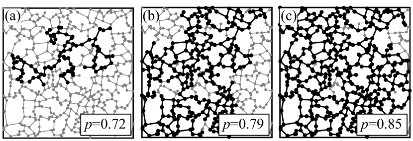
Figure 1: Bond percolation on an instance of a relative neighborhood graph for a planar set of $N=512$ points. The subfigures relate to a fraction $p$ of occupied edges, where (a) $p=0.72$ (sub-critical), (b) $p=0.79$ (close to the critical point), and (c) $p=0.85$ (super-critical). In the subfigures, nodes and edges that comprise the largest cluster on the lattice are colored black, all other nodes and edges are colored grey.

As pointed out above, percolation on the DT of a given point set in the plane is well understood. The respective thresholds for site and bond percolation can, e.g., be found under Ref. Wikipedia (2012). Regarding the subgraph hierarchy ${\rm MST}\subset{\rm RNG}\subset{\rm DT}$, the question which subgraph of the DT still features a nontrivial percolation transition was addressed recently, see Ref. Billiot et al. (2010). Intuitively, for the MST, the site and bond percolation thresholds are $1$, i.e. the transition points are trivial. Considering the RNG for a planar set of points and using the so called “method of the rolling ball”, Ref. Billiot et al. (2010) established the existence of nontrivial site and bond percolation thresholds by analytic means. However, numerical estimates for the transition points are not provided in the latter reference. Here, to elaborate on that, we perform numerical simulations in order to determine the thresholds of bond and site percolation on Euclidean RNGs for planar sets of points. Since the RNGs are subgraphs of DTs we can expect that the critical exponents that characterize the percolation transition on RNGs equal the exponents of standard $2D$ percolation. The transition is hence expected to be in the $2D$ percolation universality class and we are primarily interested in the site and bond percolation thresholds on Euclidean RNGs.

The remainder of the presented article is organized as follows. In section II, we introduce RNGs and the algorithm we use in order to compute them in more detail. In section III, we report on the numerical simulations and the analysis of the topological and percolation properties of RNGs. Section IV concludes with a summary.

II Model and Algorithm

RNGs $G=(V,E)$ are based on the concept of relative closeness. The nodeset of a $N$-point RNG is given by a set of $N$ distinct $d$-dimensional points, i.e. $V=\{p_{1},p_{2},\ldots,p_{N}\}$, where $p_{i}=(p_{i,1},\ldots,p_{i,d})$. Further, consider a metric $L_{r}$ under which for two points $p_{i}$ and $p_{j}$ the distance measure $d_{r}(p_{i},p_{j})$ is given by

$$d_{r}(p_{i},p_{j})=\big{[}\sum\nolimits_{m=1}^{d}|p_{i,m}-p_{j,m}|^{r}\big{]}^{1/r}.$$ (1)

Then, the edgeset $E$ of the RNG is obtained by connecting two points $p_{i}$ and $p_{j}$ using an undirected edge $\{p_{i},p_{j}\}$ if they are at least as close to each other as to any third point $p_{k}$, see Fig. 2(a). Hence, in order to get joined by an edge, the distance $d_{r}(p_{i},p_{j})$ of the two points has to satisfy the relation

$$d_{ij}\equiv d_{r}(p_{i},p_{j})\leq{\rm max}[d_{r}(p_{i},p_{k}),d_{r}(p_{j},p_{k})]$$ (2)

for all $k=1\ldots N$, $k\neq i,j$. If Eq. 2 is satisfied, then the two nodes are said to be relatively close. In geometrical terms, for each pair $p_{i}$ and $p_{j}$ of points, the respective distance $d_{ij}$ can be used to construct the lune ${\rm lune}(p_{i},p_{j})$. The lune is given by the intersection of two $d$-dimensional hyperspheres with equal radius $d_{ij}$ (with respect to the prevailing metric), which are centered at $p_{i}$ and $p_{j}$. If no other point $p_{k}\in V\setminus\{p_{i},p_{j}\}$ lies within ${\rm lune}(p_{i},p_{j})$, i.e. if the lune is empty, Eq. 2 holds and $p_{i}$ and $p_{j}$ are thus relatively close. In the remainder of the article, if not stated explicitly, we consider sets of points in dimension $d=2$ for the Euclidean metric $L_{2}$.

For a planar set of three points $(p_{1},p_{2},p_{3})\equiv(i,j,k)$, the above “selection criterion” for RNG-edges is illustrated in Fig. 2(a). Therein, the individual lunes are shown as shaded regions. Since ${\rm lune}(i,j)$ (encompassed by a dashed line) and ${\rm lune}(j,k)$ (encompassed by a dotted line) enclose no further point, the respective pairs of nodes are joined by undirected edges. Only ${\rm lune}(i,k)$ (encompassed by a solid line) is not empty. It encloses the point $j$, hence the points $i$ and $k$ are not joined by an undirected edge. The resulting RNG is thus $G=(V=\{i,j,k\},E=\{\{i,j\},\{j,k\}\})$. So as to facilitate intuition, a slightly less trivial example involving $N=30$ points is shown in Figs. 2(b-c). In subfigure 2(b), the RNG is highlighted as subgraph of the DT, and, in subfigure 2(c), the MST is indicated as subgraph of the RNG.

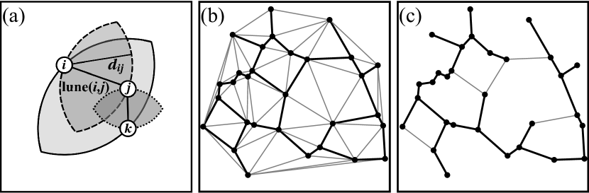
Figure 2: Illustration of the Euclidean relative neighborhood graph (RNG) and its relation to the Denlaunay triangulation (DT) and minimum-weight spanning-tree (MST) for the same set of points. (a) In a RNG, two points, say $i\equiv p_{i}$ and $j\equiv p_{j}$, are connected by an undirected edge if no third point lies within ${\rm lune}(i,j)$ (see text for more details). Further, a slightly less trivial example for $N=30$ points, showing (b) the RNG (black edges) as spanning subgraph of the DT (black and grey edges), and, (c) the MST (black edges) as spanning subgraph of the RNG (black and grey edges).

Note that a straight-forward implementation of the above RNG characteristics can be achieved by considering each pair of points (of which there are $O(N^{2})$) and checking whether one of the remaining $N-2$ points lies within their lune to rule out that they are RNG neighbors. This, however, yields an algorithm with running time $O(N^{3})$, referred to as ALG-1 by Ref. Toussaint (1980) (however, note that a tremendous speed-up can be achieved by realizing that already a single point within a given lune is sufficient to rule out that the respective lune-defining points are RNG-neighbors. Hence, as soon as for the lune of a particular pair of points the first such “intruder” is identified, one might safely proceed to the next pair of points).

For the planar case and for the Euclidean metric a more efficient algorithm, termed ALG-2 (see Ref. Toussaint (1980)), can be devised. Based on the observation that under the above assumptions the RNG is a subgraph of the DT, ALG-2 can be summarized by the following two steps: (i) construct the DT $G_{\rm DT}=(V_{\rm DT},E_{\rm DT})$ for the planar set $V$ of points, and, (ii) prune the edgeset $E_{\rm DT}$ of the DT by deleting all $\{p_{i},p_{j}\}\in E_{\rm DT}$ for which ${\rm lune}(p_{i},p_{j})$ is not empty. The latter cleanup phase then results in the edgeset $E$ of the RNG for the underlying pointset. So as to compute the DT of $V$ in step (i) above, we use the Qhull computational geometry library qHu (the DT for a set of $N$ points can be computed in time $O(N\log(N))$ Preparata and Shamos (1985); qHu ). For the implementation of step (ii) we use the “cell-list” method. Therein, the unit square, within which the $N$ points are distributed uniformly at random, is subdivided into $L\times L$ cells (where $L=\sqrt{N}$), and the $2D$ cell-indices $(i_{1},i_{2})=(\lfloor L\cdot p_{i,1}\rfloor,\lfloor L\cdot p_{i,2}\rfloor)$ for all points $p_{i}\in V$ are determined. Each cell then is equipped with a list of the points it contains. If the lune of a particular pair $\{p_{i},p_{j}\}$ of points then needs to be checked for emptiness, only a small number $n_{ij}$ of cells close to the cells with indices $(i_{1},i_{2})$ and $(j_{1},j_{2})$ have to be addressed to reach all candidate points. Note that the number $n_{ij}$ of cells to be checked depends on the precise distance $d_{ij}$ between the respective points. Typically, for large $N$, $n_{ij}$ is small for points located in the “bulk” of the unit square, and $n_{ij}$ can be rather large for points that are located along the circumference of the convex hull of $V$. The speed-up achieved by the cell-method is quite impressive, yielding an improved algorithm ALG-2-CELL that terminates in time $O(N\log(N))$. This is illustrated in Fig. 3(a), where for small systems of size $N<200$ the average running time $\langle t_{N}\rangle$ (averaged over $500$ $N$-point instances) is shown. The solid line indicated in the figure is a fit to a function of the form $\langle t_{N}\rangle\propto N\log(N)$. However, note that for $N$ not too small the data also fits well to an effective power-law function that increases $\propto N^{1.28(2)}$.

Subsequently, we will use ALG-2-CELL to compute the Euclidean RNG for $2D$ sets of points and we compute the bond and site percolation thresholds on these graphs.

Figure 3: Finite-size scaling analysis for (a) the average running time $\langle t_{N}\rangle$ of the RNG algorithm for comparatively small system sizes $N=12\ldots 192$, (b) the main plot shows the average degree $\langle k_{N}\rangle$ of the RNG nodes, and the inset illustrates the power-law correction to the scaling behavior of the average RNG diameter $\langle R_{N}\rangle$.

III Results

In the current section we will use ALG-2-CELL to compute the Euclidean RNG for planar sets of $N=144(=12^{2})\ldots 36864(=192^{2})$ points, where results are averaged over $2000$ independent RNG instances. In subsect. III.1, we report on some topological properties of RNGs and then we compute the bond and site percolation thresholds on these graphs. The data analysis for the respective bond percolation problem is discussed in detail in subsect. III.2, and the discussion for the site percolation problem in subsect. III.3 is kept more brief. A visual account of bond percolation on an instance of a $N=512$ RNG, i.e. a $2D$ system of effectively $L\times L$ points, is given in Fig. 1(a-c).

III.1 Topological properties of planar RNGs

First, we discuss two topological characteristics of RNGs, namely the average node degree and diameter (i.e. the longest among all shortest paths) of the RNG in the limit $N\to\infty$. Bear in mind that the nodes of a $N$-point RNG are distributed uniformly at random in the unit square. Thus, one might expect that the scaling behavior of observables in a $2D$ RNG depends on the effective system length $L=N^{1/2}$.

Average degree of the RNG:

The scaling behavior of the average degree $\langle k_{N}\rangle$ as function of the RNG size $N$ is shown in Fig. 3(b). Therein, the solid line indicates a fit to the function $\langle k_{N}\rangle=k_{\infty}-aN^{-b}$ where we find the asymptotic average degree $k_{\infty}=2.5576(3)$, $a=1.85(5)$, and $b=0.503(5)$ for a reduced chi-square value $\chi^{2}_{\rm red}=0.76$ (considering $n_{\rm dof}=6$ degrees of freedom).

Table 1: Critical properties that characterize bond and site percolation (BP and SP, respectively) on Euclidean RNGs for planar sets of points. From left to right: Critical point $p_{c}$ (obtained from the analysis of the Binder ratio), critical exponents $\nu$ and $\beta$ obtained from the order parameter, and $\gamma$, obtained from the order parameter fluctuations and the scaling behavior of the average size of the finite clusters for BP and SP, respectively.

Type	$p_{c}$	$\nu$	$\beta$	$\gamma$
RNG-BP	0.771(2)	1.33(6)	0.15(2)	2.40(6)
RNG-SP	0.796(2)	1.33(6)	0.14(3)	2.39(7)

Average diameter of the RNG:

The average diameter $\langle R_{N}\rangle$ of the RNG as function of $N$ is summarized in the inset of Fig. 3(b). For a planar graph like the RNG one can already expect the approximate scaling behavior $\langle R_{N}\rangle\propto N^{1/2}$. Upon analysis we found that the data fits best to a function of the form $\langle R_{N}\rangle=R_{0}N^{1/2}[1+bN^{-\omega/2}]$, where $\omega$ indicates a correction-to-scaling exponent. We estimate $R_{0}=1.75(2)$, $b=0.42(1)$, and $\omega=0.32(3)$ for a reduced chi-square value $\chi^{2}_{\rm red}=1.64$ (considering $n_{\rm dof}=6$ degrees of freedom). In the inset of Fig. 3(b) we aimed to extract the correction to scaling according to $\langle R_{N}\rangle N^{-1/2}-R_{0}\propto N^{-\omega/2}$ . The numerical value of $R_{0}$ can also be set into a context Toussaint (1980): for the MST on has $\langle R_{N}^{\rm MST}\rangle=R_{0}^{\rm MST}N^{1/2}$, where $0.5\leq R_{0}^{\rm MST}\leq 0.707$, see Refs. Gilbert (1965); Roberts (1968). Since the RNG is a supergraph of the MST one thus might expect to find $R_{0}\geq R_{0}^{\rm MST}$.

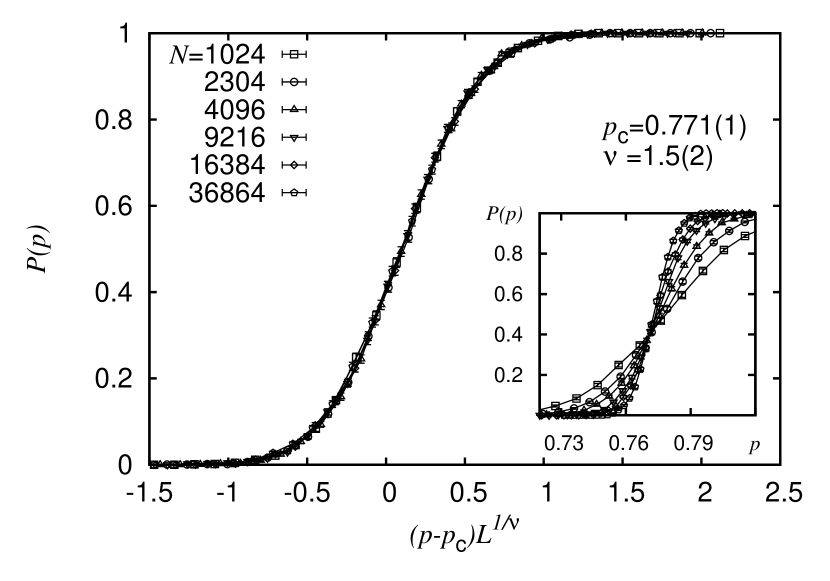
Figure 4: Finite-size scaling analysis of the bond percolation probability $P(p)$ (i.e. the probability of simultaneous percolation along both independent directions; see text) on RNGs for planar sets of $N=1024\ldots 36864$ points, averaged over $2000$ different graph instances. The main plot shows the data collapse obtained using Eq. 3, and the inset illustrates the raw data close to the critical point.

III.2 Results for bond percolation on planar RNGs

To simulate the bond-percolation problem on instances of RNGs we implemented the highly efficient, union-find based algorithm due to Newman and Ziff, see Ref. Newman and Ziff (2000, 2001). Therein, initially, each node comprises its own (single-node) cluster. We proceed by choosing edges from $E$, one after the other, in random order. For each edge we check whether its terminal nodes belong to different clusters. If this is the case, the respective clusters are merged using the “union-by-size” approach. Once all edges are considered, the particular RNG instance is completed. In principle, this allows to compute observables very efficiently with a resolution of $O(1/|E|)$. For a more clear presentation, and so as to be able to compute proper errorbars for the observables below, we consider $2000$ independent RNG instances for a given value of $N$ and approximately $80$ supporting points on the $p$ axis (in the vicinity of the critical point) for which averages are computed. The observables we consider below can be rescaled following a common scaling assumption. Below, this is formulated for a general observable $y(p,L)$. This scaling assumption states that if the observable obeys scaling, it can be rewritten as

$$y(p,L)=L^{-b}~{}f[(p-p_{c})L^{1/\nu}],$$ (3)

wherein $\nu$ and $b$ represent dimensionless critical exponents (or ratios thereof, see below), $p_{c}$ signifies the critical point, and $f[\cdot]$ denotes an unknown scaling function. Following Eq. 3, data curves of the observable $y(p,L)$ recorded at different values of $p$ and $L$ collapse, i.e. fall on top of each other, if $y(p,L)L^{b}$ is plotted against the combined quantity $\epsilon\equiv(p-p_{c})L^{\nu}$ and if further the scaling parameters $p_{c}$, $\nu$ and $b$ that enter Eq. 3 are chosen properly. The values of the scaling parameters that yield the best data collapse determine the numerical values of the critical exponents that govern the scaling behavior of the underlying observable $y(p,L)$. In order to obtain a data collapse for a given set of data curves we here perform a computer assisted scaling analysis, see Refs. Houdayer and Hartmann (2004); Melchert (2009). The resulting numerical estimates of the critical thresholds and exponents for bond and site percolation on planar Euclidean RNGs are listed in Tab. 1. In the subsequent paragraphs, we report on the results found for different observables.

Percolation probability:

In order to provide a measure of percolation probability for the $2D$ RNG, we proceed as follows: For each instance of a $N$-point RNG we first determine the $L$ points that are closest to the left, right, top, and bottom boundary. As a sufficient condition for percolation along, say, the horizontal direction, we consider the event that a point on the left and the right boundary are part of the same cluster. Here, we put under scrutiny the particular event that the system simultaneously percolates along both independent directions (other criteria yield similar results). The finite-size scaling analysis of the corresponding percolation or “spanning” probability $P(p)$ is summarized in Fig. 4. Setting $b=0$ in Eq. 3 (as appropriate for a dimensionless quantity) and restricting the analysis to the interval $\epsilon=[-0.5,0.5]$ on the rescaled $p$-axis, we find that $p_{c}=0.771(1)$ and $\nu=1.5(2)$ yield a best data collapse with “collapse-quality” $S=0.33$ (the numerical value of $S$ measures the mean–square distance of the data points to the master curve, described by the scaling function, in units of the standard error Houdayer and Hartmann (2004)). Note that the numerical value of the correlation length exponent is in agreement with the standard $2D$ percolation exponent $\nu=4/3\approx 1.333$.

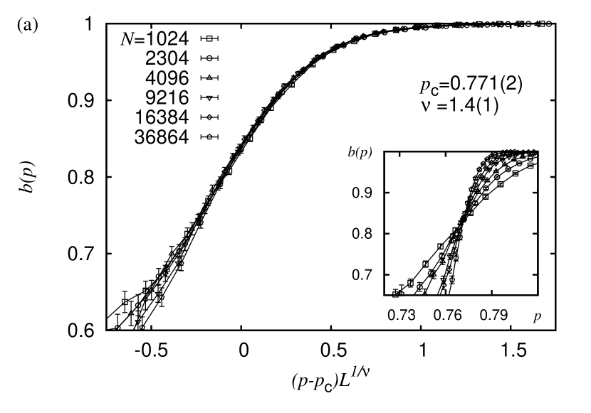
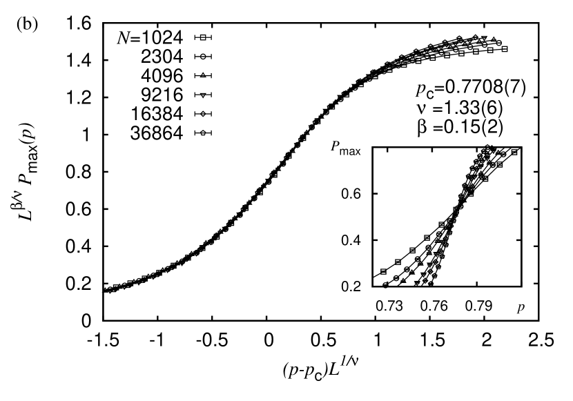
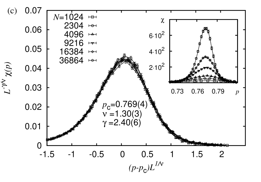
Figure 5: Finite-size scaling analyses related to the relative size $s_{\rm max}$ of the largest cluster of sites on RNGs for planar sets of $N=1024\ldots 36864$ points, averaged over $2000$ graph instances. The main plots show the data collapse obtained according to Eq. 3, and the insets illustrate the raw data close to the critical point. The subfigures show different ways to analyze $s_{\rm max}$ in terms of (a) the Binder ratio $b(p)$, (b) the order parameter $s_{\rm max}(p)$, and, (c) the fluctuation $\chi(p)=N{\rm var}(s_{\rm max})$ of the order parameter.

Order parameter statistics:

As a second observable we consider $s_{\rm max}$, i.e. the relative size of the largest cluster of points joined by edges. In this regard, a further dimensionless quantity commonly referred to in the analysis of phase transitions is the Binder ratio Binder (1981)

$$b(p)=\frac{1}{2}\Big{[}3-\frac{\langle s_{\rm max}^{4}(p)\rangle}{\langle s_{\rm max}^{2}(p)\rangle^{2}}\Big{]}.$$ (4)

This ratio of moments scales according to Eq. (3), where, as for the spanning probability above, $b=0$. As can be seen from the inset of Fig. 5(a), the Binder ratio exhibits a nice common crossing point of the data curves for different values of $N$. The best data collapse (obtained in the (unsymmetrical) range $\epsilon\in[-0.1,1.0]$) yields $p_{c}=0.772(2)$, and $\nu=1.4(2)$ with a quality $S=1.22$. As evident from the rescaled data (main plot of Fig. 5(a)), there are rather strong deviations from the expected scaling behavior as $p<p_{c}$. To account for this, the scaling analysis is performed in the rather unsymmetrical interval $\epsilon\in[-0.1,1.0]$ on the rescaled $p$-axis to accentuate the region $p>p_{c}$ where $b(p)$ seems to scale well. As above, the numerical value of the exponent $\nu$ is in agreement with the standard $2D$ percolation exponent. Considering the order parameter

$$P_{\rm max}(p)=\langle s_{\rm max}(p)\rangle,$$ (5)

the best data collapse (obtained in the range $\epsilon\in[-1,1]$) yields $p_{c}=0.7708(7)$, $\nu=1.33(6)$, and $\beta=0.15(2)$ with a quality $S=0.50$, see Fig. 5(b)). If we fix the numerical values of the critical exponents to the expected values $\nu=4/3\approx 1.333$ and $\beta=5/36\approx 0.139$ we are left with only one adjustable parameter, resulting in the estimate $p_{c}=0.7711(6)$ with $S=0.88$. A further critical exponent can be estimated from the scaling of the order parameter fluctuations $\chi(p)$, given by

$$\chi(p)=N[\langle s_{\rm max}^{2}(p)\rangle-\langle s_{\rm max}(p)\rangle^{2}].$$ (6)

A best data collapse for this observable (attained in the range $\epsilon\in[-0.2,0.2]$) results in the estimates $p_{c}=0.769(4)$, $\nu=1.30(3)$, and $\gamma=2.40(6)$ with a quality $S=0.24$, see Fig. 5(c). Note that the numerical value of the fluctuation exponent is in agreement with the expected value $\gamma=43/18\approx 2.389$.

Average size of the finite clusters:

As a last observable we consider the average size $\langle S_{\rm fin}(p)\rangle$ of all finite clusters for a particular RNG, averaged over different instances of RNGs. The respective definition reads Sur et al. (1976); Stauffer and Aharony (1994)

$$S_{\rm fin}(p)=\frac{\sum_{s}^{\prime}s^{2}\,n_{s}(p)}{\sum_{s}^{\prime}s\,n_{s}(p)},$$ (7)

where $n_{s}(p)$ signifies the probability mass function of cluster sizes for a single RNG instance at a given value of $p$. Note that the sums run over finite clusters only Sur et al. (1976); Stauffer and Aharony (1994) (indicated by the prime), i.e. if the precise configuration features a system spanning cluster (spanning horizontally or vertically or both), this cluster is excluded from the sums that enter Eq. 7. The average size of all finite clusters is expected to scale according to Eq. 3, where $b=-\gamma/\nu$. Restricting the data analysis to the interval $\epsilon\in[-1.0,1.0]$ on the rescaled $p$-axis, the optimal scaling parameters are found to be $p_{c}=0.770(2)$, $\nu=1.36(4)$, and $\gamma=2.33(5)$ with a quality $S=0.61$ (not shown). Note that here, the numerical values of the extracted exponents are in reasonable agreement with the expected values and the estimate of the critical threshold for bond percolation is consistent with the numerical values found above.

III.3 Results for site percolation on planar RNGs

The analysis in terms of the site percolation problem was carried out analogous to that of the bond percolation problem in the preceding subsection. However, we here list only the estimates of the critical points obtained from the data collapse analysis for the different observables. In this regard we have $p_{c}=0.799(1)$ (percolation probability), $p_{c}=0.796(2)$ (Binder ratio), $p_{c}=0.795(1)$ (order parameter), $p_{c}=0.794(4)$ (order parameter fluctuation; see Tab. 1), $p_{c}=0.798(3)$ (average size of the finite clusters). Further, the critical exponents $\nu=1.33(6)$ and $\beta=0.14(3)$ obtained from the order parameter and $\gamma=2.39(7)$, obtained from the scaling behavior of the average size of the finite clusters, are listed in Tab. 1.

IV Discussion and summary

In the presented article we have closely investigated the statistical and percolation properties of planar Euclidean RNGs via numerical simulations. In regard of the subgraph hierarchy $MST\subset RNG\subset DT$, recently the question was raised which subgraph of the DT (on which the percolation problem is well studied) still features a nontrivial percolation transition Billiot et al. (2010). Intuitively, for the MST this is not the case. For the RNG previous analytic studies established the existence of nontrivial site and bond percolation thresholds Billiot et al. (2010), but no numerical estimates where provided. Here we quote $p_{c,{\rm bond}}^{\rm RNG}=0.771(2)$ and $p_{c,{\rm site}}^{\rm RNG}=0.796(2)$, obtained by means of finite-size scaling analyses in terms of the “data-collapse” technique. Further, we also deduced the critical exponents that govern both percolation transitions on the RNG and found them to be consistent with those that describe the standard $2D$ percolation phenomenon (as expected). So as to yield maximally justifiable results through numerical redundancy, we considered various observables to estimate the critical points and exponents.

As discussed in subsect. III.1, the asymptotic average degree for the RNG reads $k_{\infty}=2.5576(3)$. In order to put the above critical points into a context, we might attempt to compare them to the threshold values for regular $2D$ lattices with a similar degree. E.g., the site and bond percolation thresholds for the ($3$,$12^{2}$)-Archimedean lattice, having degree $k=3$, read $p_{c,{\rm bond}}=0.74042081(10)$ Ziff and Gu (2009) and $p_{c,{\rm site}}=0.807900764\ldots$ Suding and Ziff (1999). Both are actually not thus far from the respective thresholds on the RNG. (Further, for the $k=3$ Martini lattice one has $p_{c,{\rm bond}}=0.707107\ldots$ Ziff (2006) and $p_{c,{\rm site}}=0.764826\ldots$ Scullard (2006).) Regarding $2D$ random lattices, site and bond percolation on the Voronoi tesselation of a planar pointset, also having degree $k=3$, give rise to the threshold values $p_{c,{\rm bond}}=0.666931(5)$ and $p_{c,{\rm site}}=0.71410(2)$ Becker and Ziff (2009). In addition, site percolation on planar $\Phi^{3}$ random graphs result in $p_{c,{\rm site}}=0.7360(5)$ Kownacki (2008). In comparison, the estimates from the latter random graphs are less close to the estimates for the RNG as compared to the ($3$,$12^{2}$)-Archimedean lattice thresholds.

As pointed out in the introduction, RNGs are discussed in the context of the construction of planar “virtual backbones” for ad-hoc networks that guarantee connectedness of all considered nodes Karp and Kung (2000); Bose et al. (2001); Jennings and Okino (2004); Yi et al. (2010). In this regard, from a point of view of stability, it would be interesting to quantify how susceptible RNGs are with respect to a random failure and targeted removal of nodes and to compare the results to other “proximity graph” instances which are discussed in the same context. Such investigations are currently underway Melchert et al. (2012).