Chiral Perturbation Theory and Mesons

Abstract:

The talk contains a short introduction to mesonic Chiral Perturbation Theory (ChPT). In addition four disparate areas where some progress has been made in recent years are discussed. These are the last fit of the order $p^{4}$ low-energy-constants $L_{i}^{r}$ to data, hard pion ChPT, the recent two-loop work on EFT for QCD like theories and the high order leading logarithm calculations in the massive $O(N)$ nonlinear sigma model.

1 Introduction

This talk is dedicated to my friend and collaborator Ximo Prades who died since the previous Chiral Dynamics in Berne in 2009. For those of you who like to know more I recommend looking up the slides from my talk at the symposium in Granada in his memory [1]. We have been very frequent collaborators for a long time.

I will not attempt to give an overview of Chiral Perturbation Theory (ChPT) for mesons in this talk. Even with the restrictions to mesons the subject is very large. I have given several review talks earlier [2, 3] as well as written a review article of mesonic ChPT at two-loop order [4]. References to other reviews and lectures can be found on my ChPT webpage [5], the remainder there has admittedly a strong bias towards my own work.

I will give a short introduction to ChPT where I emphasize the major ideas underlying the method. Afterwards I will give an overview of the work that has been happening in Lund in this area in the last few years. In addition there are many more talks at this conference related to mesonic ChPT. As far as the plenary talks are concerned these are the experimental tests from NA48 [6] and KLOE [7], the connection with dispersion relations [8, 9] and the connection with lattice QCD [10, 11, 12]. Most of the talks in the working group on Goldstone Bosons also fall under the topic of this talk.

The remainder is first a short introduction to ChPT, then an overview of the latest fit of the low-energy-constants, a few remarks about hard-pion-ChPT as well as some comments about applications of ChPT beyond QCD and some leading logarithm calculations to high orders. The treatment is extremely cursory for all cases.

2 Chiral Perturbation Theory

ChPT in its modern form was introduced by Weinberg [13], and Gasser and Leutwyler [14, 15]. The best way to characterize ChPT is:

Exploring the consequences of the chiral symmetry of QCD and its spontaneous breaking using effective field theory techniques

A good reference that shows in detail all the underlying assumptions is [16].

For an effective field theory, one needs to indicate three things: the relevant degrees of freedom, a power-counting principle to have predictivity and the associated range of validity. For ChPT these are

Degrees of freedom:

The Goldstone Bosons from the spontaneous breaking of the chiral symmetry present in QCD in the massless limit.

Power-counting:

Dimensional counting in momenta and masses where meson masses and momenta are counted the same in the standard counting.

Range of validity:

The breakdown scale is when effects that are not included become important. For mesonic ChPT these are clearly the meson resonances in the relevant channels. $M_{\rho}$ is thus clearly the end of the range.

Let me show these now in a little more detail. Quantum Chromodynamics (QCD) for $n_{F}$ equal mass quarks has an obvious global symmetry under the continuous interchange of the quarks $SU(n_{F})$. Looking at the purely strong Lagrangian (density)

$${\cal L}_{QCD}=\sum_{q=u,d,s}\left[i\bar{q}_{L}D\hskip-5.59721pt/\,q_{L}+i\bar{q}_{R}D\hskip-5.59721pt/\,q_{R}-m_{q}\left(\bar{q}_{R}q_{L}+\bar{q}_{L}q_{R}\right)\right],$$ (1)

we see that in the limit of $m_{q}=0$ there is actually the larger $SU(n_{F})\times SU(n_{F})_{R}$ global symmetry. Another way to see is that in the massless case left- and right-handed are no longer related by Lorentz-transformations since we cannot go the rest-frame of a massless particle.

The global chiral symmetry $SU(3)_{L}\times SU(3)_{R}$ in QCD is spontaneously broken to the vector subgroup $SU(3)_{V}$ by the vacuum expectation value $\langle\bar{q}q\rangle=\langle\bar{q}_{L}q_{R}+\bar{q}_{R}q_{L}\rangle\neq 0$. Since in this process 8 generators are broken we get 8 Goldstone Bosons and their interactions vanish at zero momentum. This is shown pictorially for one broken generator in Fig. 2.

\begin{overpic}[width=113.81102pt,unit=0.5pt]{broken.eps} \SetScale{0.5} \SetWidth{2.} \SetColor{Red} \LongArrow(105,60)(180,20) \end{overpic}

Figure 1: We need to pick a vacuum expectation value indicated by the arrow. The massless mode corresponds to an excitation along the bottom of the valley.

rules:                                    one loop example:

$p^{2}$

$1/p^{2}$

$\int d^{4}p$ $p^{4}$

$(p^{2})^{2}\,(1/p^{2})^{2}\,p^{4}=p^{4}$ $(p^{2})\,(1/p^{2})\,p^{4}=p^{4}$

Figure 2: An example of the power-counting, on the left the rules for the lowest order vertex, propagator and loop integration. On the right showing how it leads to the two one-loop diagrams being $p^{4}$ while the tree level lowest-order vertex is $p^{2}$.

The fact that the interaction vanishes at zero momentum allows us to introduce a proper power-counting along the lines discussed in [13]. This is shown for the example of $\pi\pi$-scattering at one loop in Fig. 2.

The basic principle just described has been used in very many circumstances. One needs to decide which chiral perturbation theory is appropriate for the problem at hand. Some examples are

• Which chiral symmetry: $SU(N_{f})_{L}\times SU(N_{f})_{R}$, for $N_{f}=2,3,\ldots$ and extensions to (partially) quenched

• Or beyond QCD

• Space-time symmetry: Continuum or broken on the lattice: Wilson, staggered, mixed action

• Volume: Infinite, finite in space, finite T

• Which interactions to include beyond the strong one

• Which particles included as non Goldstone Bosons

• My general belief: if it involves soft pions (or soft $K,\eta$) some version of ChPT exists.

An important technical step is the inclusion of external fields or sources. This allows to make the chiral symmetry local [14, 15]. The manifold at the bottom of the potential in a symmetry breakdown $SU(n_{F})_{L}\times SU(n_{F})\times SU(n_{F})_{V}$ is also an $SU(n_{F})$ manifold. We thus parametrize this by an $n_{F}\times n_{F}$ matrix which for $n_{F}=3$ is

$$U(\phi)=\exp(i\sqrt{2}\Phi/F_{0}),\quad\mathrm{with}\quad\Phi(x)=\,\left(\begin{array}[]{ccc}\displaystyle\frac{\pi^{0}}{\sqrt{2}}\,+\,\frac{\eta_{8}}{\sqrt{6}}&\pi^{+}&K^{+}\\ \pi^{-}&\displaystyle-\frac{\pi^{0}}{\sqrt{2}}\,+\,\frac{\eta_{8}}{\sqrt{6}}&K^{0}\\ K^{-}&\bar{K}^{0}&\displaystyle-\frac{2\,\eta_{8}}{\sqrt{6}}\end{array}\right).$$ (2)

The lowest-order (LO) Lagrangian is

$${\cal L}_{2}=\frac{F_{0}^{2}}{4}\{\langle D_{\mu}U^{\dagger}D^{\mu}U\rangle+\langle\chi^{\dagger}U+\chi U^{\dagger}\rangle\}\,,$$ (3)

with the covariant derivative $D_{\mu}U=\partial_{\mu}U-ir_{\mu}U+iUl_{\mu}\,,$ and the left and right external currents/fields/sources: $r(l)_{\mu}=v_{\mu}+(-)a_{\mu}$. The scalar and pseudo-scalar external densities are include via $\chi=2B_{0}(s+ip).$ The latter allow the inclusion of quark masses via the scalar density: $s={\cal M}+\cdots$. The notation implies a flavour trace $\langle A\rangle=Tr_{F}\left(A\right)$. The next-to-leading-order (NLO) Lagrangian was worked out by Gasser and Leutwyler [14, 15] and has 10+2 terms. The next-to-next-to-leading-order (NNLO) Lagrangian is also known [17] as well as its infinities [18]. The number of terms is summarized in Tab. 1.

2 flavour 3 flavour 3+3 PQChPT $p^{2}$ $F,B$ 2 $F_{0},B_{0}$ 2 $F_{0},B_{0}$ 2 $p^{4}$ $l_{i}^{r},h_{i}^{r}$ 7+3 $L_{i}^{r},H_{i}^{r}$ 10+2 $\hat{L}_{i}^{r},\hat{H}_{i}^{r}$ 11+2 $p^{6}$ $c_{i}^{r}$ 52+4 $C_{i}^{r}$ 90+4 $K_{i}^{r}$ 112+3

Table 1: The number of terms at LO [19], NLO [14, 15]and NNLO [17] for standard mesonic ChPT.

All the cases listed above have extra terms in the Lagrangian with the exception of finite volume and temperature and in most cases the Lagrangian is known to NLO. The constants in the Lagrangian are often referred to as low-energy-constants (LECs).

So, what does ChPT really predict given the large number of free constants. It relates processes with different numbers of pseudo-scalars and includes isospin and the eightfold way ($SU(3)_{V}$). The chiral logarithms can be seen in the two-flavour ChPT NLO expression for the pion mass[14]

$$m_{\pi}^{2}=2B\hat{m}+\left(\frac{2B\hat{m}}{F}\right)^{2}\left[\frac{1}{32\pi^{2}}{\log\frac{\left(2B\hat{m}\right)}{\mu^{2}}}+2l_{3}^{r}(\mu)\right]+\cdots$$ (4)

with $M^{2}=2B\hat{m}$ and remember that $B\neq B_{0}$, $F\neq F_{0}$, the constants in two and three flavour ChPT are not necessarily the same. The chiral logarithm is the $\log(2B\hat{m})$ term. The infinities are treated by the relation between the bare and renormalized couplings and the renormalized couplings do depend on the renormalization scale $\mu$ and the scheme used.

In two-flavour ChPT [14] one uses conventionally the quantities $\bar{l}_{i}=\frac{32\pi^{2}}{\gamma_{i}}\,l_{i}^{r}(\mu)-\log\frac{M_{\pi}^{2}}{\mu^{2}}\,.$ which are independent of the scale $\mu$. For 3 and more flavours, some of the $\gamma_{i}$ are zero and one uses the renormalized constants $L_{i}^{r}({\mu})$ directly. The result is in principle independent of $\mu$ but when estimating some of the constants some choices might be better than others. The most standard value is $\mu=m_{\rho}=0.77$ GeV since if we choose $\mu\approx m_{\pi}$, $m_{K}$ the chiral logarithms vanish and if we pick a larger scale of about 1 GeV then $L_{5}^{r}(\mu)\approx 0$ and arguments using a large number of colours, $N_{c}\to\infty$ are strongly violated.

A question which often comes up is in which quantities to expand, in particular whether to use lowest-order or physical quantities. I would like to stress here that the expansion is in momenta and masses but that it is not unique. There simply is no best way to do the expansion since relations between the masses, e.g. the Gell-Mann–Okubo relation, exist. But even more, often there are relations between the kinematical quantities and masses. An example is $\pi K$ scattering with $s+t+u=m_{\pi}^{2}+m_{K}^{2}$, or one can even use the scattering angle as a kinematical quantity. A related note is that there can be remaining $\mu$-dependence in a calculation where the $\mu$-dependence is then higher order. A naive example was discussed in the talk and can be found in [20] showing that the apparent convergence of the chiral series can differ very much depending on what quantities one expands in. In general, I prefer using the physical masses since thresholds are correct and the chiral logarithms do come from physical particles propagating. However, sometimes there are simply too many choices of physical masses possible, especially in partially quenched and staggered ChPT, and for the sake of simplicity it might be easier to keep lowest-order masses everywhere.

3 Determining low-energy-constants in the continuum

Lattice QCD has now reached the stage where they can start determining the ChPT LECs. A review is the FLAG collaboration [21] and talks at this conference that had results on LECS are [10, 22, 23, 24].

For the two-flavour constants the status has not really changed much since the previous chiral dynamics. The constants $\bar{l}_{1}$ to $\bar{l}_{4}$ are determined from ChPT at order $p^{6}$ and the Roy equation analysis in $\pi\pi$ and $F_{S}$ [25]. A related talk is [26]. $\bar{l}_{5}$ and $\bar{l}_{6}$ come from $F_{V}$ and $\pi\to\ell\nu\gamma$ [27, 28] and from $\Pi_{V}-\Pi_{A}$ [29]. Some related work using similar sum rules is [30]. In conclusion:

$$\bar{l}_{1} =-0.4\pm 0.6\,, \bar{l}_{2} =4.3\pm 0.1\,, \bar{l}_{3} =2.9\pm 2.4\,,$$

$$\bar{l}_{4} =4.4\pm 0.2\,, \bar{l}_{5} =12.24\pm 0.21\,, \bar{l}_{6}-\bar{l}_{5} =3.0\pm 0.3\,,$$

$$\bar{l}_{6} =16.0\pm 0.5\pm 0.7\,.$$

and $l_{7}\sim 5\cdot 10^{-3}$ from $\pi^{0}$-$\eta$ mixing [14]. In the two-flavour case the contribution from the order $p^{6}$ LECs was small so the uncertainty on estimating those is not very important.

The uncertainty on estimates of the order $p^{6}$ LECs, the $C_{i}^{r}$, in the three flavour case is much more important because $m_{K}^{2},m_{\eta}^{2}\gg m_{\pi}^{2}$. The larger $C_{i}^{r}$ dependent contributions make their estimates much more relevant. Typically, if the term multiplying a particular $C_{i}^{r}$ leads to a kinematical dependence it can be measured and the estimates tested. But if it leads only to a higher order quark-mass dependence they lead to experiment in a 100% correlated way with the order $p^{4}$ LECs, the $L_{i}^{r}$. Here we really need the lattice, typically the latter type of $C_{i}^{r}$ need scalars to estimate their values from resonance exchance and are thus intrinsically less well estimated. In addition, often the large $N_{c}$ suppressed terms in the order $p^{6}$ lagrangian contribute with large coefficients as well and all estimates so far of the LECs rely on large $N_{c}$ to a large extent. One big question is thus whether we are really testing ChPT or simply doing a phenomenological fit. In order to answer this question a systematic search for relations that are independent of the $C_{i}^{r}$ was done [31]. We found there 35 relations between 76 observables and of these 13 had sufficient data to study their success. There were 7 relations in $\pi\pi$ scattering which worked about the same for two and three flavour ChPT. The two relations involving $a_{3}^{-}$ did not work well in either case. Of the 5 extra relations involving $\pi\pi$ and $\pi K$ scattering three worked well, one of the bad ones involved $a_{3}^{-}$ and the last one had very large NNLO corrections. The final relation involves $K_{\ell 4}$ and did not work well probably because ChPT fails to describe the quadratic slope in the $F$ form-factor [32, 33]. The quality of the relations is shown in Fig. 3. The conclusion is that three flavour ChPT “sort of” works taking into account that the relations involve very large correlations and that thus the experimental or dispersive input errors might be underestimated.

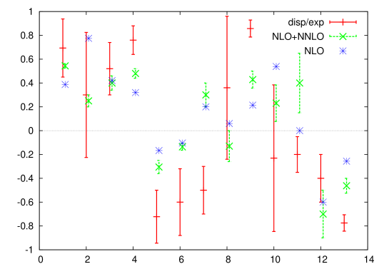
Figure 3: The quality of the relations found in [31]. Shown are the NLO and NNLO predictions for combinations of observables with vanishes NNLO LEC contributions as well as the experimental/dispersive results for the same combinations.

The previous major fit to determine the $L_{i}^{r}$ using NNLO formulas dates back to 2001 [34]. Given that many more calculations in three flavour ChPT at NNLO have been performed since and that the experimental input used then has also changed, an update has become necessary. This was done in [35] and the main results are summarized in Tab. 2.

fit 10 iso NA48/2 $F_{K}/F_{\pi}$ All $\star$ All old data $\pi\pi$, $\pi K$, $\langle r_{S}^{2}\rangle$ $m_{s}/\hat{m}$ $10^{3}L_{1}^{r}$ $0.39\pm 0.12$ $0.88$ $0.87$ $0.89$ $0.88\pm 0.09$ $10^{3}L_{2}^{r}$ $0.73\pm 0.12$ $0.79$ $0.80$ $0.63$ $0.61\pm 0.20$ $10^{3}L_{3}^{r}$ $-2.34\pm 0.37$ $-3.11$ $-3.09$ $-3.06$ $-3.04\pm 0.43$ $10^{3}L_{4}^{r}$ $\equiv 0$ $\equiv 0$ $\equiv 0$ $0.60$ $0.75\pm 0.75$ $10^{3}L_{5}^{r}$ $0.97\pm 0.11$ $0.91$ $0.73$ $0.58$ $0.58\pm 0.13$ $10^{3}L_{6}^{r}$ $\equiv 0$ $\equiv 0$ $\equiv 0$ $0.08$ $0.29\pm 0.85$ $10^{3}L_{7}^{r}$ $-0.30\pm 0.15$ $-0.30$ $-0.26$ $-0.22$ $-0.11\pm 0.15$ $10^{3}L_{8}^{r}$ $0.60\pm 0.20$ $0.59$ $0.49$ $0.40$ $0.18\pm 0.18$ $\chi^{2}$ $0.26$ $0.01$ $0.01$ $1.20$ $1.28$ dof 1 1 1 4 4

Table 2: The main new fit of the $L_{i}^{r}$ of [35]. The various columns show the changes w.r.t. the old fit of [34].

The old programs in the isospin conserving versions were rewritten in C++ for this purpose. The first column uses the old input values and reproduces the old fit [34] which was done isospin violation included. The next columns give the results from including the NA48/2 data on the form factors [36], the new value of $F_{K}/F_{\pi}$, the inclusion of $\pi\pi$, $\pi K$ scattering and the scalar radius and finally the new value of $m_{s}/\hat{m}$. The LEC that changed most at each step is put in a box. In the final result one note significant values for the $N_{c}$-suppressed constants $L_{4}^{r},L_{6}^{r}$, albeit with large errors and the fact the the large $N_{c}$-relation $2L_{1}^{r}=L_{2}^{r}$ no longer holds well.

A large number of variations on the fit were tried in [35] by letting $\mu$ free and varying the input used for the $C_{i}^{r}$. All of these gave similar values for the $L_{i}^{r}$. However, a problem occurred when including the relation between the 2 and 3-flavour LECs of [37]. In order for getting this relation to work well we needed nonzero values for at least some $N_{c}$-suppressed $C_{i}^{r}$. In [35] a large effort was done to find reasonable looking $C_{i}^{r}$ that allowed to get good fits to all of the inputs. Many were found but there is no good ground to prefer any of these. More work especially in trying to include lattice results is definitely needed. For now, fit All of Tab. 2 and [35] should be regarded as the standard values for the $L_{i}^{r}$.

4 Hard pion ChPT

The usual formulation of the powercounting in mesonic ChPT [13] assumes that all the momenta in all diagrams are soft and this allows the powercounting to work as simple dimensional counting. In baryon and heavy meson ChPT one takes a step further. There is a line with a heavy mass running through all diagrams but in a way all spatial momenta can still be considered small. In vector meson ChPT it has been argued that it is possible to also include diagrams where lines take a hard momentum, but not a hard mass [38]. This type of arguments was used by Flynn and Sachrajda [39] to obtain results for $K_{\ell 3}$ in the heavy Kaon limit also away from the end-point. These arguments, as described below were generalized and applied to a larger number of processes in [40, 41, 42, 43]. Some doubt on the simple arguments has been presented in [44, 45].

The underlying idea behind hard pion ChPT is that nonanalyticities in the the light masses, e.g. pion, come from soft lines in the diagrams. The couplings of soft particles and in particular soft pions are constrained by current algebra via

$$\lim_{q\to 0}\langle\pi^{k}(q)\alpha|O|\beta\rangle=-\frac{i}{F_{\pi}}\langle\alpha|\left[Q_{5}^{k},O\right]|\beta\rangle\,,$$ (5)

and nothing prevents hard pions to be present in the states $|\alpha\rangle$ or $|\beta\rangle$. One thus expects that by heavily using current algebra it should be possible to obtain chiral logarithms for almost any process. one can always expand in soft momenta over hard momenta/large masses in a way which is analogous to the treatment of infrared divergences in QED. The general argument was already described in my previous chiral dynamics talk [3] and can be found in [40, 41, 42] as well. It roughly goes as follows: Take any diagram with a particular external and internal momentum configuration. Identify the soft lines and cut them. The resulting part is analytic in the soft stuff and should thus be describable by an effective Lagrangian with coupling constants dependent on the external given momenta (Weinberg’s folklore theorem [13]) Lagrangian in hadron fields with all orders of derivatives. This effective Lagrangian should be thought of as a Lagrangian in hadron fields but all possible orders of the momenta included: possibly an infinite number of terms If symmetries are present, the Lagrangian should respect them. The problem is that the simple power-counting is gone In some cases we can argue that up to a certain order in the expansion in light masses, not momenta, matrix elements of higher order operators are reducible to those of lowest order, first done in [39] for $K_{\ell 3}$ and later generalized. The Lagrangian should be complete in the neighbourhood of the original process and loop diagrams with this effective Lagrangian should reproduce the non-analyticities in the light masses. The latter is the crucial part of the argument.

A check at two-loop order has been performed for the pion vector and scalar form-factor in [41, 42] and was found to work well. Applications to the $B,D\to\pi,K,\eta$ vector form-factors can be found in [42] and to some charmonium decays in [43]. In Fig. 4 I show how the inclusion of the chiral logarithms improves the relation between the $D\to\pi$ and $D\to K$ form-factors [42] using the CLEO data [46].

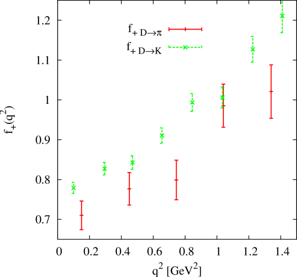
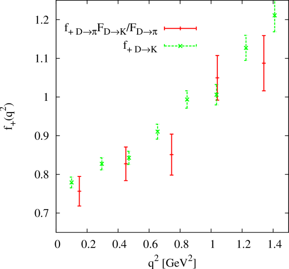
Figure 4: The left plot shows the form-factor $f_{+}$ in $D\to\pi e\nu$ and $D\to Ke\nu$ decays from CLEO [46]. In the right hand side the $D\to Ke\nu$ has been corrected with the chiral logarithms via $f_{+D\to\pi}=f_{+D\to K}F_{D\to\pi}/F_{D\to K}$ [42].

Recently [44, 45], the test done at two loops was extended to higher orders. What was found there was that the hard pion ChPT prediction held to all orders for the elastic intermediate state but failed in a three loop calculation of the inelastic four-particle-cut part. For details I refer to [44, 45]. The arguments for the general method are the same as for IR divergences, SCET,…, so I do believe these to be valid. Something like hard pion ChPT should exist. The arguments for the proportionality to the lowest order are much weaker and assume that each soft propagator has a free momentum. The calculation of [45] was done using dispersive methods and a full calculation at 3 loops will be very difficult but would allow a better study of why the arguments failed. The ultimate would of course be to find a proper power-counting under the given assumptions.

5 Beyond QCD

The methods of effective field theory and in particular ChPT can also be used for extensions. A simple extension is to take QCD with $N$ light flavours but one can also envisage using $N$ fermions in different representations of the gauge group. The representations can be complex, real or pseudo-real so we have in general three generic cases to study for the spontaneous breaking of the global symmetries [47, 48]

$$SU(N)\times SU(N)\to SU(N),\quad SU(2N)\to SO(2N),\quad SU(2N)\to Sp(2N)\,.$$ (6)

The cases correspond to a complex, real and pseudo-real representation for the $N$ fermions. The global symmetry group in the latter two cases is $SU(2N)$ since both fermion and antifermion are in the same representation of the gauge group. Many one-loop results existed especially for the first case, the equal mass case has been pushed to two-loop order in [49, 50, 51]. The main observation [49] is that the whole machinery developed for ChPT can be brought over with a few simple modifications to the three cases given above. This allowed us to perform the calculations for the mass and decay constants [49], meson-meson scattering [50] and the electroweak precision parameters [51]. The main idea was that lattice calculation can use our formulas to extrapolate to the massless case, see e.g. [52].

The main trick involved is that in all cases mesons can be described by a unitary matrix $U=\exp(i\phi^{a}X^{a}/(\sqrt{2}F))$ with the $X^{a}$ a different set of generators for the three cases. All flavour sums in the equal mass case can be done using the relations

$$\langle X^{a}AX^{a}B\rangle =\langle A\rangle\langle B\rangle-\frac{1}{N_{F}}\langle AB\rangle\,, \langle X^{a}A\rangle\langle X^{a}B\rangle =\langle AB\rangle-\frac{1}{N_{F}}\langle A\rangle\langle B\rangle\,.$$

$$\langle X^{a}AX^{a}B\rangle =\frac{\langle A\rangle\langle B\rangle}{2}+\frac{1}{2}\langle AJ_{S}B^{T}J_{S}\rangle-\frac{\langle AB\rangle}{2N_{F}}\,, \langle X^{a}A\rangle\langle X^{a}B\rangle =\frac{1}{2}\langle AB\rangle+\frac{1}{2}\langle AJ_{S}B^{T}J_{S}\rangle-\frac{\langle A\rangle\langle B\rangle}{2N_{F}}\,.$$

$$\langle X^{a}AX^{a}B\rangle =\frac{\langle A\rangle\langle B\rangle}{2}+\frac{1}{2}\langle AJ_{A}B^{T}J_{A}\rangle-\frac{\langle AB\rangle}{2N_{F}}\,, \langle X^{a}A\rangle\langle X^{a}B\rangle =\frac{1}{2}\langle AB\rangle-\frac{1}{2}\langle AJ_{A}B^{T}J_{A}\rangle-\frac{\langle A\rangle\langle B\rangle}{2N_{F}}.$$ (7)

The lines are for the complex, real and pseudo-real case and $J_{S}=\left(\begin{array}[]{cc}0&I\\ I&0\end{array}\right)$, $J_{A}=\left(\begin{array}[]{cc}0&-I\\ I&0\end{array}\right)$.

As an example I quote the results for the vacuum expectation value $\langle\bar{q}q\rangle$ for all three cases.

$$\langle\overline{q}q\rangle =\langle\overline{q}q\rangle_{\mathrm{LO}}+\langle\overline{q}q\rangle_{\mathrm{NLO}}+\langle\overline{q}q\rangle_{\mathrm{NNLO}}\,.$$

$$\langle\overline{q}q\rangle_{\mathrm{LO}} \equiv\sum_{i=1,N_{F}}\langle\overline{q}_{Ri}q_{Li}+\overline{q}_{Li}q_{Ri}\rangle_{\mathrm{LO}}=-N_{F}B_{0}F^{2}$$

$$\langle\overline{q}q\rangle_{\mathrm{NLO}} =\langle\overline{q}q\rangle_{\mathrm{LO}}\left(a_{V}\frac{\overline{A}(M^{2})}{F^{2}}+b_{V}\frac{M^{2}}{F^{2}}\right)\,,$$

$$\langle\overline{q}q\rangle_{\mathrm{NNLO}} =\langle\overline{q}q\rangle_{\mathrm{LO}}\Bigg{(}c_{V}\frac{\overline{A}(M^{2})^{2}}{F^{4}}+\frac{M^{2}\overline{A}(M^{2})}{F^{4}}\left(d_{V}+\frac{e_{V}}{16\pi^{2}}\right)+\frac{M^{4}}{F^{4}}\left(f_{V}+\frac{g_{V}}{16\pi^{2}}\right)\Bigg{)}\,.$$ (8)

I used here $M^{2}=2B_{0}\hat{m}$ and $\overline{A}(M^{2})=-\frac{M^{2}}{16\pi^{2}}\log\frac{M^{2}}{\mu^{2}}\,.$ The coefficients appearing are given in Tab. 3. Note the similarity between the different results and the existence of a number of large $n$ relations between the various cases [49].

	QCD	Adjoint	2-colour
$a_{V}$	$n-\frac{1}{n}$	$n+\frac{1}{2}-\frac{1}{2n}$	$n-\frac{1}{2}-\frac{1}{2n}$
$b_{V}$	$16nL_{6}^{r}+8L_{8}^{r}+4H_{2}^{r}$	$32nL_{6}^{r}+8L_{8}^{r}+4H_{2}^{r}$	$32nL_{6}^{r}+8L_{8}^{r}+4H_{2}^{r}$
$c_{V}$	$\frac{3}{2}\left(-1+\frac{1}{n^{2}}\right)$	$\frac{3}{8}\left(-1+\frac{1}{n^{2}}-\frac{2}{n}+2n\right)$	$\frac{3}{8}\left(-1+\frac{1}{n^{2}}+\frac{2}{n}-2n\right)$
$d_{V}$	$-24\left(n^{2}-1\right)\,\left(L_{A}+\frac{L_{B}}{n}\right)$	$-12\left(2n^{2}+n-1\right)\left(2L_{A}+\frac{L_{B}}{n}\right)$	$-12\left(2n^{2}-n-1\right)\left(2L_{A}+\frac{L_{B}}{n}\right)$
$e_{V}$	$1-\frac{1}{n^{2}}$	$\frac{1}{4}\left(1-\frac{1}{n^{2}}+\frac{2}{n}-2n\right)$	$\frac{1}{4}\left(1-\frac{1}{n^{2}}-\frac{2}{n}+2n\right)$
$f_{V}$	$48\left(K_{25}^{r}+nK_{26}^{r}+n^{2}K_{27}^{r}\right)$	$r^{r}_{VA}$	$r^{r}_{VT}$
$g_{V}$	$8\left(n^{2}-1\right)\,\left(L_{A}+\frac{1}{n}L_{B}\right)$	$4\left(2n^{2}+n-1\right)\left(2L_{A}+\frac{1}{n}L_{B}\right)$	$4\left(2n^{2}-n-1\right)\left(2L_{A}+\frac{1}{n}L_{B}\right)$

Table 3: The coefficients appearing the corrections to the vacuum-expectation-value for the three generic cases with $n$ flavours. Table from [49]. We have defined the abbreviations $L_{A}=L_{4}^{r}-2L_{6}^{r}$ and $L_{B}=L_{5}^{r}-2L_{8}^{r}$.

6 Leading logarithms

The last part on which I want to report is some recent progress in calculating leading logarithms in effective field theories. Some of this is also mentioned in the talk by Kampf [53]. The underlying argument goes something like: Take a quantity with a single scale: $F(M)$. The dependence on the scale in field theory is typically logarithmic, so with $L=\log\left(\mu/M\right)$we get

$$F=F_{0}+F_{1}^{1}{L}+F^{1}_{0}+F_{2}^{2}{L^{2}}+F^{2}_{1}L+F^{2}_{0}+F_{3}^{3}{L^{3}}+\cdots$$ (9)

The leading logarithms are the terms with $F_{m}^{m}{L^{m}}$. The $F_{m}^{m}$ can be more easily calculated than the full result. This follows from the fact that for any physical quantity $\mu\left(dF/d\mu\right)\equiv 0$ and ultraviolet divergences in Quantum Field Theory are always local. In renormalizable theories this is embedded in the renormalization group but for effective field theories such as QCD there is no simple recursive argument. Weinberg already argued that one can get away with only one-loop calculations to obtain the leading logarithms [13]. This was proven in [54] and in a somewhat simpler way in [55]. The underlying reason is that the cancellation of nonlocal divergences gives a set of consistency relations between contributions of different loop order as explained in [56]. In the massless case [57, 58, 59] this leads to an almost analytic expression to very high orders since the diagrams remain fairly simple to all orders. In the massive case diagrams with any number of external legs show up but the whole process can be automatized since in [55] it was realized that the Lagrangians at higher order do not need to be minimal. Obtaining the minimal Lagrangian at each order would have been essentially impossible. In the massive case all published results relate to the $O(N)$ model, masses in [55], decay constants and vacuum expectation values as well as form-factors and meson-meson scattering in [60] and the anomalous sector [61]. Extension to $SU(N)\times SU(N)$ has been done in the massless case [59] and is in progress for the massive case. I refer to the original papers for more results but a few highlights are that the large $N$ (number of flavours) limit is not a good approximation for any of the quantities calculated. The series seem to converge in the expected regions. None of the leading logarithms calculated seems to be unusually large. Unfortunately the hope that we might recognize the general result for arbitrary $N$ proved in vain.

- [1] Symposium in memory of professor Ximo Prades, http://www.ugr.es/~fteorica/Ximo/.
- [2] J. Bijnens, Status of Strong ChPT, \posPoS(EFT09)022 [arXiv:0904.3713 [hep-ph]].
- [3] J. Bijnens, Chiral perturbation theory in the meson sector, \posPoS(CD09)031 [arXiv:0909.4635 [hep-ph]].
- [4] J. Bijnens, Chiral perturbation theory beyond one loop, Prog. Part. Nucl. Phys. 58 (2007) 521 [hep-ph/0604043].
- [5] J. Bijnens, http://home.thep.lu.se/~bijnens/chpt/.
- [6] A. Bizzetti, \posPoS(CD12)003.
- [7] F. Bossi, \posPoS(CD12)011.
- [8] S. Lanz, \posPoS(CD12)007.
- [9] I. Caprini, \posPoS(CD12)006.
- [10] L. Lellouch, \posPoS(CD12)008.
- [11] C. Sachrajda, \posPoS(CD12)009.
- [12] T. Izubuchi, \posPoS(CD12)026.
- [13] S. Weinberg, Phenomenological Lagrangians, Physica A 96 (1979) 327.
- [14] J. Gasser and H. Leutwyler, Chiral Perturbation Theory to One Loop, Annals Phys. 158 (1984) 142.
- [15] J. Gasser and H. Leutwyler, Chiral Perturbation Theory: Expansions in the Mass of the Strange Quark, Nucl. Phys. B 250 (1985) 465.
- [16] H. Leutwyler, On the foundations of chiral perturbation theory, Annals Phys. 235 (1994) 165 [hep-ph/9311274].
- [17] J. Bijnens, G. Colangelo and G. Ecker, The Mesonic chiral Lagrangian of order , JHEP 9902 (1999) 020 [hep-ph/9902437].
- [18] J. Bijnens, G. Colangelo and G. Ecker, Renormalization of chiral perturbation theory to order , Annals Phys. 280 (2000) 100 [hep-ph/9907333].
- [19] S. Weinberg, Nonlinear realizations of chiral symmetry, Phys. Rev. 166 (1968) 1568.
- [20] J. Bijnens, Quark Mass dependence at Two Loops for Meson Properties, PoS LAT 2007 (2007) 004 [arXiv:0708.1377 [hep-lat]].
- [21] G. Colangelo, et al., Review of lattice results concerning low energy particle physics, Eur. Phys. J. C 71 (2011) 1695 [arXiv:1011.4408 [hep-lat]].
- [22] E. Stolz, \posPoS(CD12)055.
- [23] A. Deuzeman, \posPoS(CD12)034.
- [24] C. Bernard, \posPoS(CD12)030.
- [25] G. Colangelo, J. Gasser and H. Leutwyler, pi pi scattering, Nucl. Phys. B 603 (2001) 125 [hep-ph/0103088]
- [26] G. Rios, \posPoS(CD12)051.
- [27] J. Bijnens, G. Colangelo and P. Talavera, The Vector and scalar form-factors of the pion to two loops, JHEP 9805 (1998) 014 [hep-ph/9805389].
- [28] J. Bijnens and P. Talavera, form-factors at two loop, Nucl. Phys. B 489 (1997) 387 [hep-ph/9610269].
- [29] M. Gonzalez-Alonso, A. Pich and J. Prades, Determination of the Chiral Couplings L(10) and C(87) from Semileptonic Tau Decays, Phys. Rev. D 78 (2008) 116012 [arXiv:0810.0760 [hep-ph]].
- [30] J. Bordes, C. A. Dominguez, P. Moodley, J. Penarrocha and K. Schilcher, Chiral corrections to the Gell-Mann-Oakes-Renner relation, JHEP 1005 (2010) 064 [arXiv:1003.3358 [hep-ph]].
- [31] J. Bijnens and I. Jemos, Relations at Order in Chiral Perturbation Theory, Eur. Phys. J. C 64 (2009) 273 [arXiv:0906.3118 [hep-ph]].
- [32] G. Amoros, J. Bijnens and P. Talavera, form-factors and scattering, Nucl. Phys. B 585 (2000) 293 [Erratum-ibid. B 598 (2001) 665] [hep-ph/0003258].
- [33] P. Stoffer, \posPoS(CD12)058.
- [34] G. Amoros, J. Bijnens and P. Talavera, QCD isospin breaking in meson masses, decay constants and quark mass ratios, Nucl. Phys. B 602 (2001) 87 [hep-ph/0101127].
- [35] J. Bijnens and I. Jemos, A new global fit of the at next-to-next-to-leading order in Chiral Perturbation Theory, Nucl. Phys. B 854 (2012) 631 [arXiv:1103.5945 [hep-ph]].
- [36] J. R. Batley et al. [NA48-2 Collaboration], Precise tests of low energy QCD from -decay properties, Eur. Phys. J. C 70 (2010) 635.
- [37] J. Gasser, C. Haefeli, M. A. Ivanov and M. Schmid, Integrating out strange quarks in ChPT, Phys. Lett. B 652 (2007) 21 [arXiv:0706.0955 [hep-ph]].
- [38] J. Bijnens, P. Gosdzinsky and P. Talavera, Matching the heavy vector meson theory, JHEP 9801 (1998) 014 [hep-ph/9708232].
- [39] J. M. Flynn et al. [RBC and UKQCD Collaborations], SU(2) chiral perturbation theory for -decay amplitudes, Nucl. Phys. B 812 (2009) 64 [arXiv:0809.1229 [hep-ph]].
- [40] J. Bijnens and A. Celis, Decays in SU(2) Chiral Perturbation Theory, Phys. Lett. B 680 (2009) 466 [arXiv:0906.0302 [hep-ph]].
- [41] J. Bijnens and I. Jemos, Hard Pion Chiral Perturbation Theory for and Formfactors, Nucl. Phys. B 840 (2010) 54 [Erratum-ibid. B 844 (2011) 182] [arXiv:1006.1197 [hep-ph]].
- [42] J. Bijnens and I. Jemos, Vector Formfactors in Hard Pion Chiral Perturbation Theory, Nucl. Phys. B 846 (2011) 145 [arXiv:1011.6531 [hep-ph]].
- [43] J. Bijnens and I. Jemos, Chiral Symmetry and Charmonium Decays to Two Pseudoscalars, Eur. Phys. J. A 47 (2011) 137 [arXiv:1109.5033 [hep-ph]].
- [44] M. Procura, \posPoS(CD12)049.
- [45] G. Colangelo, M. Procura, L. Rothen, R. Stucki and J. Tarrus Castella, On the factorization of chiral logarithms in the pion form factors, JHEP 1209 (2012) 081 [arXiv:1208.0498 [hep-ph]].
- [46] J. Y. Ge et al. [CLEO Collaboration], Study of , and in Tagged Decays of the Resonance, Phys. Rev. D 79 (2009) 052010 [arXiv:0810.3878 [hep-ex]].
- [47] M. E. Peskin, The Alignment of the Vacuum in Theories of Technicolor, Nucl. Phys. B 175 (1980) 197.
- [48] J. Preskill, Subgroup Alignment in Hypercolor Theories, Nucl. Phys. B 177 (1981) 21.
- [49] J. Bijnens and J. Lu, Technicolor and other QCD-like theories at next-to-next-to-leading order, JHEP 0911 (2009) 116 [arXiv:0910.5424 [hep-ph]].
- [50] J. Bijnens and J. Lu, Meson-meson Scattering in QCD-like Theories, JHEP 1103 (2011) 028 [arXiv:1102.0172 [hep-ph]].
- [51] J. Bijnens and J. Lu, Two-Point Functions and S-Parameter in QCD-like Theories, JHEP 1201 (2012) 081 [arXiv:1111.1886 [hep-ph]].
- [52] M. Buchoff, \posPoS(CD12)031.
- [53] K. Kampf, \posPoS(CD12)039.
- [54] M. Buchler and G. Colangelo, Renormalization group equations for effective field theories, Eur. Phys. J. C 32 (2003) 427 [hep-ph/0309049].
- [55] J. Bijnens and L. Carloni, Leading Logarithms in the Massive O(N) Nonlinear Sigma Model, Nucl. Phys. B 827 (2010) 237 [arXiv:0909.5086 [hep-ph]].
- [56] J. Bijnens, G. Colangelo, G. Ecker, J. Gasser and M. E. Sainio, Pion pion scattering at low-energy, Nucl. Phys. B 508 (1997) 263 [Erratum-ibid. B 517 (1998) 639] [hep-ph/9707291].
- [57] N. Kivel, M. V. Polyakov and A. Vladimirov, Chiral Logarithms in the Massless Limit Tamed, Phys. Rev. Lett. 101 (2008) 262001 [arXiv:0809.3236 [hep-ph]].
- [58] N. A. Kivel, M. V. Polyakov and A. A. Vladimirov, Leading Chiral Logarithms for Pion Form Factors to Arbitrary Number of Loops, JETP Lett. 89 (2009) 529 [arXiv:0904.3008 [hep-ph]].
- [59] J. Koschinski, M. V. Polyakov and A. A. Vladimirov, Leading Infrared Logarithms from Unitarity, Analyticity and Crossing, Phys. Rev. D 82 (2010) 014014 [arXiv:1004.2197 [hep-ph]].
- [60] J. Bijnens and L. Carloni, The Massive O(N) Non-linear Sigma Model at High Orders, Nucl. Phys. B 843 (2011) 55 [arXiv:1008.3499 [hep-ph]].
- [61] J. Bijnens, K. Kampf and S. Lanz, Leading logarithms in the anomalous sector of two-flavour QCD, Nucl. Phys. B 860 (2012) 245 [arXiv:1201.2608 [hep-ph]].