Assessing the Constrained Harmonic Mean Method for Deriving the Kinematics of ICMEs with a Numerical Simulation

Abstract

In this study we use a numerical simulation of an artificial coronal mass ejection (CME) to validate a method for calculating propagation directions and kinematical profiles of interplanetary CMEs (ICMEs). In this method observations from heliospheric images are constrained with in-situ plasma and field data at 1 AU. These data are used to convert measured ICME elongations into distance by applying the Harmonic Mean approach that assumes a spherical shape of the ICME front. We use synthetic white-light images, similar as observed by STEREO-A/HI, for three different separation angles between remote and in-situ spacecraft, of $30^{\circ}$, $60^{\circ}$, and $90^{\circ}$. To validate the results of the method they are compared to the apex speed profile of the modeled ICME, as obtained from a top view. This profile reflects the “true” apex kinematics since it is not affected by scattering or projection effects. In this way it is possible to determine the accuracy of the method for revealing ICME propagation directions and kinematics. We found that the direction obtained by the constrained Harmonic Mean method is not very sensitive to the separation angle ($30^{\circ}$ sep: $\phi=$ W7; $60^{\circ}$ sep: $\phi=$ W12; $90^{\circ}$ sep: $\phi=$ W15; true dir.: E0/W0). For all three cases the derived kinematics are in a relatively good agreement with the real kinematics. The best consistency is obtained for the $30^{\circ}$ case, while with growing separation angle the ICME speed at 1 AU is increasingly overestimated ($30^{\circ}$ sep: $\Delta V_{\rm arr}\approx-50$ km s^-1, $60^{\circ}$ sep: $\Delta V_{\rm arr}\approx+75$ km s^-1, $90^{\circ}$ sep: $\Delta V_{\rm arr}\approx+125$ km s^-1). Especially for future L₄/L₅ missions the $60^{\circ}$ separation case is highly interesting in order to improve space weather forecasts.

1 Introduction

s:intro

Coronal Mass Ejections (CMEs) are the most powerful eruptions on the Sun and are currently observed by a relatively large number of instruments. Space-based coronagraphs are located at three different positions to monitor the solar corona from all sides. SOlar and Heliospheric Observatory (SOHO) LASCO coronagraphs (C2 and C3: Brueckner et al., 1995) at L₁ provide white-light images up to a distance of 32 R_⊙. The two spacecraft of the Solar TErrestrial RElations Observatory (STEREO: Kaiser et al., 2008) move apart by $45^{\circ}$ per year and are currently at a position of more than $120^{\circ}$ eastern and western from Earth, respectively. As part of the Sun-Earth Connection Coronal and Heliospheric Investigation suite (SECCHI: Howard et al., 2008; Harrison et al., 2009) the COR1 and COR2 coronagraphs aboard the two spacecraft STEREO-A and STEREO-B provide continuous white-light observations up to 15 R_⊙. Combining coronagraphs with the Heliospheric Imagers HI1 and HI2 (Eyles et al., 2009), which are also part of the SECCHI suite aboard STEREO, the entire propagation of an ICME from Sun to 1 AU is covered. Both HIs are off-pointed from the center of the Sun and cover a field of view (FoV) of $4^{\circ}$ to $24^{\circ}$ and $18.7^{\circ}$ to $88.7^{\circ}$ elongation, respectively.

Such wide FoVs make the interpretation of extended structures in these images rather difficult and Thomson scattering effects (Billings, 1966; Hundhausen, 1993) as well as effects due to line of sight (LoS) integration have to be taken into account. Methods were developed in order to investigate the propagation of CMEs beyond the typical FoV of coronagraph images, which are up to about $4^{\circ}$ (COR2) or $9^{\circ}$ (LASCO C3) elongation. These methods are based on specific geometrical assumptions about the shape of the ICME front. Some assume a point-like structure as the Fixed-$\phi$ method (F$\phi$: Sheeley et al., 1999; Rouillard et al., 2008) or the triangulation method developed by Liu et al. (2010) that uses stereoscopic observations. The Harmonic Mean method (Lugaz, 2010) and the Self Similar Expansion method (Davies et al., 2012) assume a circular front. Fixed-$\phi$, Harmonic Mean (Lugaz, 2010; Möstl et al., 2011) and the Self Similar Expansion method (Möstl and Davies, 2012) are also used as fitting methods by assuming constant ICME speed and direction. In this way, these methods can be used to forecast the ICME arrival at 1 AU. An alternative forecasting tool is the drag based model, developed by Vršnak et al. (2012). It is based on the idea that the aerodynamic drag in the ambient medium is responsible for the adjustment of the ICME speed to the solar wind speed.

ICMEs are not only remotely observed but also measured in-situ, among others, from both STEREO spacecraft (IMPACT: Luhmann et al., 2008), from Wind (Ogilvie et al., 1995) and the Advanced Composition Explorer (ACE: Stone et al., 1998). ACE and Wind are both located at the L₁ point. In order to guard against misunderstandings, we use the term ICME as defined by Rouillard (2011), i.e. an ICME includes the shock (if present), the dense sheath region and the magnetic flux rope. Furthermore we use this term for white-light observations beyond the coronagraphic FoV as well as for the in-situ structure. Using plasma and magnetic field data from in-situ observations, in addition to remote sensing of ICMEs, we are able to constrain the results derived from measurements of white-light images (Möstl et al., 2009a, 2010; Rollett et al., 2012). In the following we refer to the method as “constrained” Harmonic Mean method (CHM). The kinematical profiles resulting from the CHM method may also be compared to the results of the drag based model and serve for studies of the interaction of ICMEs with solar wind strucures (Temmer et al., 2011, 2012).

MHD simulations of ICMEs evolving in interplanetary (IP) space have already been used to validate the Fixed-$\phi$ fitting and Harmonic Mean fitting methods (Lugaz, Roussev, and Gombosi, 2011). By using synthetically derived ICME density images and time-elongation plots (Jmaps: Davies et al., 2009), measured from different viewing angles, we aim to validate the CHM method and present a detailed error analysis in order to improve the forecasting of Earth-directed ICMEs. We construct the Jmaps for different separation angles between the remote and the in-situ spacecraft observing the ICME, namely $30^{\circ}$, $60^{\circ}$, and $90^{\circ}$. The $60^{\circ}$ case is in particular interesting, as it simulates the observational capabilities for L₄/L₅ missions, which are currently under discussion to optimize space weather predictions (Gopalswamy et al., 2011).

2 MHD Simulations

s:models

Simulations give us the opportunity to study the kinematical behavior of ICMEs from an ideal location as observer, namely top view along the Sun-Earth line, which enables us to directly measure the time-distance profile of the ICME evolution. This is in contrast to how we actually observe ICMEs, i.e. from a side view involving LoS and scattering effects, from which we measure an elongation angle that needs to be converted into radial distance by using different conversion methods. From the model we obtain both views, and use these two capabilities to test the efficiency of the CHM method to derive the kinematics of an ICME measured from synthetic Jmaps as observed by STEREO-A and to calculate ICME propagation directions. Synthetic Jmaps are produced from three different observing positions, i.e. $30^{\circ}$, $60^{\circ}$, and $90^{\circ}$ between ICME apex and remote spacecraft in order to test the influence of the observing angle to the resulting directions and kinematics.

The numerical modeling of the simulated ICME is done by using the Space Weather Modeling Framework (SWMF: Tóth et al., 2005). Along the Sun-Earth line the grids of the model vary in spatial resolution from $0.5$ R_⊙ close to the Sun to $0.25$ R_⊙ in the middle and $0.125$ R_⊙ close to Earth. Synthetic in-situ data, i.e. magnetic field, plasma density and plasma bulk velocity, are produced for the location of Earth. This is done using the semiempirical MHD model developed by Cohen et al. (2007), which applies the empirical Wang–Sheeley–Arge model (WSA: Wang and Sheeley, 1990; Arge and Pizzo, 2000) and a flux rope CME initiated at the solar surface (similar setup as in Lugaz et al., 2009b). During the last 16 hours before the shock hits Earth the temporal resolution is about 2 – 3 minutes in order to capture the details of the transition of the shock.

The modeled fictitious ICME is launched on 15 February 2011 01:00:00 into a steady state background solar wind ($V_{\rm sw}\approx 430$ km s^-1). It has a very wide angular extent within the ecliptic and is expanding to all sides. It is directed toward the virtual in-situ spacecraft at the position of Earth and the ICME apex arrives 48 hours later on 17 February 2011 01:00:00. The ICME is faster than the ambient solar wind. It decelerates from 1100 km s^-1 at 60 R_⊙ to 800 km s^-1 at 150 R_⊙, and the shock finally arrives with $\approx 650$ km s^-1 at the in-situ spacecraft.

Figure fig:insitu shows the synthetic in-situ data extracted at the position of Earth. In the upper panel the three components of the magnetic field and the total magnetic field strength (black line) are plotted in cartesian coordinates with origin in Sun-center, x- and y-axes lie in the ecliptic plane and z-axis points to the ecliptic north pole to complete the right hand triad. The middle and the bottom panel show the speed in km s^-1 and the proton number density in cm^-3, respectively. The red vertical line indicates the arrival of the shock preceding the ICME. If the shock is absent, the arrival time cannot be defined unambiguously. This could yield an additional uncertainty.

The left part of Figure fig:topjmap shows the location of the observing remote spacecraft (yellow dot) and in-situ spacecraft (red dot) as viewed from top at one time step of the ICME evolution. The black semicircle is the Thomson surface (TS: Vourlidas and Howard, 2006; Howard and DeForest, 2012) and the dashed yellow line is the LoS along the ICME front, i.e. the projection of the TS onto the ecliptic plane, from the view of the remote spacecraft for which the Jmap is produced. The corresponding Jmap is shown on the right side of Figure fig:topjmap. The bright features are the integrated signal along the LoS with its intensity maximum at the TS. The method to produce synthetic Jmaps is described in Lugaz et al. (2009b).

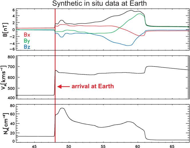
Figure 1.: Synthetic in-situ data at the position of Earth. The upper panel shows the magnetic field with its three components (cartesian coordinate system) and the total magnetic field strength, the middle panel shows the speed and the bottom panel the proton number density. The vertical red line marks the shock arrival time at Earth that is used for further calculations. The x-axis gives the time in hours from launch of the CME at the Sun.fig:insitu

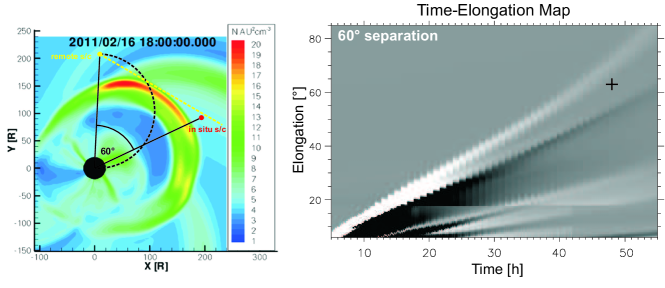
Figure 2.: Left: top view of the modeled ICME for $60^{\circ}$ separation between remote (yellow dot) and in-situ spacecraft (red dot). The black semicircle is the Thomson surface and the dashed yellow line is the LoS along the ICME front. Right: side view of the propagating ICME simulated as observed by STEREO-A/HI. The bright track shows the evolution in time of the apparent ICME front. The black cross marks the elongation of the in-situ spacecraft at shock arrival time.fig:topjmap

3 Analysis Methods

s:methods To determine the kinematical properties of an ICME, we usually measure the apparent front, either in the direct white-light images or within Jmaps. Tracking the bright features in a Jmap has two advantages. First, the contrast between dense and less dense areas can easily be seen, which enables us to track ICMEs over larger elongations, hence, radial distances. Especially in HI2 images the brightness rapidly decreases and it is hardly feasible to identify the front at larger elongations. Second, due to the shape of the track that is directly visible in the Jmap, i.e. the evolution of elongation with time, it is possible to get a first estimate of the direction of the ICME (Sheeley et al., 2008). This is used in fitting methods as the Fixed-$\phi$ fitting (Kahler and Webb, 2007; Rouillard et al., 2008) or the Harmonic Mean fitting methods (Lugaz, 2010; Möstl et al., 2011) that can also be used to predict ICME arrival times. However, these fitting methods use the assumption of constant speed, which is very useful to get a rough estimate for the direction and the arrival time of the ICME. But to analyze variations in the kinematical behavior due to interactions with e.g. high speed streams, corotating interaction regions or preceding ICMEs (e.g. Gopalswamy et al., 2001; Burlaga, Plunkett, and St. Cyr, 2002; Lugaz, Vourlidas, and Roussev, 2009a; Temmer et al., 2011, 2012) it is required to apply a method, which allows the ICME speed to vary during propagation.

Such an approach, which uses additional in-situ data to constrain measurements from white-light data, is described in Rollett et al. (2012). In this study we validate the CHM method (using the constraint of arrival time) and derive the effective error in the ICME distance–time and speed–distance profiles.

3.1 Constrained Harmonic Mean Method

In the following we briefly outline the CHM method and its main features, for more details we refer the interested reader to Rollett et al. (2012). At this point we stress that the CHM method is not a forecasting method but an approach to analyze ICMEs after they are remotely observed and measured in-situ, respectively. In this way we are able to derive a kinematical profile for the purpose of analyzing variations in speed. In order to convert the measured elongation angle [$\epsilon(t)$] into a unit of distance we use an approach assuming a circular ICME front, the so-called Harmonic Mean method (HM: Howard and Tappin, 2009; Lugaz, Vourlidas, and Roussev, 2009a). HM was shown to be a quite good approximation for very wide events. This method assumes the observer to look along the tangent to the spherical ICME front and more or less disregards the concept of the intensity maximum on the TS. Equation (eq:hmean1) shows the conversion of $\epsilon(t)$ into the radial distance of the ICME apex [$R_{\rm HM}(t)$] for a given propagation direction [$\phi$]:

$$R_{\rm HM}(t)=\frac{2d_{\rm o}\sin\epsilon(t)}{1+\sin(\epsilon(t)+\phi)},\ilabel{eq:hmean1}$$ (1)

where $d_{\rm o}$ is the Sun-observer distance. For the constraint with the in-situ arrival time we need the distance of the ICME front in the direction of the in-situ spacecraft. This is given by

$$R_{\rm HMi,t_{a}}(\phi)=R_{\rm HM,t_{a}}(\phi)\cos{\delta},\ilabel{eq:cosinus}$$ (2)

where $R_{\rm HMi,t_{a}}(\phi)$ is the distance of the ICME front in the direction of the in-situ spacecraft at arrival time [$t_{\rm a}$], $R_{\rm HM,t_{a}}$ is the distance of the ICME apex at arrival time and $\delta$ is the angle between the line of the in-situ spacecraft to the Sun [$d_{\rm i}$], and $R_{\rm HM}(t)$. To determine the propagation direction we now calculate

$$\Delta d_{\rm HMi}(\phi)=R_{\rm HMi,t_{a}}(\phi)-d_{\rm i},\ilabel{eq:rinsitu}$$ (3)

for $\phi\in[0^{\circ},180^{\circ}]$. The direction providing the minimum value for $\Delta d_{\rm HMi}(\phi)$ is the resulting propagation direction $\phi$ that is now used to convert $\epsilon(t)$ into distance by using Equation (eq:hmean1).

In other words: the input parameter $\phi$, and therefore also the shape of the distance–time profile, is changed until the best accordance with the in-situ arrival time is found. This ensures that the HI observations are consistent with the in-situ data, which serve as a boundary condition for the kinematical profiles. In addition, the input paramter $\phi$, used for the best agreement, is the calculated propagation direction of the ICME apex (Möstl et al., 2009b, 2010; Rollett et al., 2012).

3.2 Speed Calculation

When the ICME speed profile is derived from the calculated distance its shape strongly depends on the uncertainties in the distance profile. Therefore it is necessary to fit the distance profile and use this fit for further calculations. In Gallagher, Lawrence, and Dennis (2003) and Bein et al. (2011) fitting functions and methods are described for coronagraphic FoVs close to the Sun. These functions take into account the strong acceleration and deceleration at the beginning of the CME evolution (Zhang et al., 2001). Since we analyze data from HI we are mainly interested in the propagation phase, during which the ICME adjusts to the solar wind speed, and developed a function, which takes into account the different parts of the distance–profile for the HI FoV:

$$F(x)=A_{1}\ln(x)+A_{2}x+A_{3}\sqrt{x}+A_{4},\ilabel{eq:fit}$$ (4)

where the first term reproduces the strong deceleration at the beginning of the HI1 FoV, the second term describes the roughly constant speed during the propagation phase. The third term takes into account the slowly decreasing/increasing speed and is needed to avoid an overestimation of the arrival speed at 1 AU, and the constant is the y-intercept. Figure fig:fits shows the distance–time fits and the fitting parameters for all three separations. The time derivatives of the distance–time fits are over plotted on the speed–time profiles, derived from the distance measurements converted from the elongation–time profiles. The error bars show the standard deviations calculated from measuring each track five times.

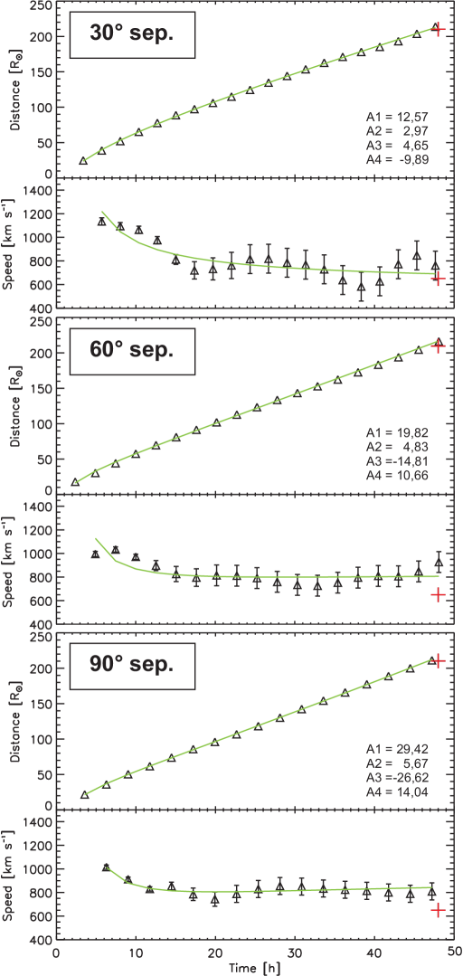
Figure 3.: Distance–time profiles with over plotted fits for $30^{\circ}$, $60^{\circ}$, and $90^{\circ}$ separation of remote and in-situ spacecraft. In each case the upper panel shows the distance measurements converted from the elongation–time profiles (triangles), the over plotted fits and the fitting parameters in R_⊙. The lower panels show the time derivatives from the distance–time profiles and the over plotted time derivatives of the distance–time fits. The red crosses mark the in-situ measured arrival time and speed, respectively.fig:fits

3.3 Error Analysis

Uncertainties in the analysis of ICME kinematics and directions are due to various reasons. By using a modeled ICME it is possible to provide an error estimation for the most significant contributions.

If the apparent front of an ICME is measured from white-light images the intensity range is varying, i.e. if a track is measured by more than one person there will be a certain spread of measurements. To quantify this error we determine an error range for the measurements by performing two surveys—one very high (outermost) and one very low (innermost) track (see Section s:kin). The mean differences between these two tracks lie between $\pm 0.3^{\circ}$ (HI1) and $\pm 1.35^{\circ}$ elongation (HI2) for all three separation cases.

To estimate the error due to visually tracking of the elongation–time profile, the Jmap track is measured five times. Out of this sample we calculate the mean values and standard deviations for every Jmap track. The elongation errors for all three separation cases lie in a range of about $\pm 0.1^{\circ}$ (HI1) and $\pm 0.4^{\circ}$ (HI2).

Table tab:error lists the mean values for the three cases of different separation angles between in-situ and remote spacecraft and both HI instruments, for the two derived errors in elongation, i.e. the intensity range, where measurements could be taken within the Jmap and the measurement error itself. For further calculations only the measurement error is taken into account. Table tab:error2 gives the errors for the resulting distance in R_⊙ and the speed in km s^-1.

We only consider errors due to the measurements itself. Uncertainties beacause of the assumed circular shape or the angular width of the ICME front are not taken into account. Since HM assumes a width of $180^{\circ}$ it may not be the right approach for narrow events. In this case the F$\phi$ method should provide more reliable results.

Table 1.: Summary of calculated errors denoted in elongation for each separation case and each heliospheric instrument: HI1 and HI2. The first row lists the standard deviation of the innermost and the outermost Jmap track, i.e. the possible Jmap tracking area. The second row shows the measurement error derived out of the five tracks in elongation.tab:error

	$30^{\circ}$ separation		$60^{\circ}$ separation		$90^{\circ}$ separation
	HI1	HI2	HI1	HI2	HI1	HI2
Jmap tracking area	$\pm 0.25^{\circ}$	$\pm 1.35^{\circ}$	$\pm 0.3^{\circ}$	$\pm 1^{\circ}$	$\pm 0.3^{\circ}$	$\pm 0.7^{\circ}$
mean standard deviation	$\pm 0.1^{\circ}$	$\pm 0.4^{\circ}$	$\pm 0.5^{\circ}$	$\pm 1.9^{\circ}$	$\pm 0.5^{\circ}$	$\pm 1.4^{\circ}$

Table 2.: Resulting errors for the ICME kinematics. The first row lists the distance error in R_⊙ based on the mean standard deviations for both instruments. The second row shows the speed error derived from the standard deviations.tab:error2

	$30^{\circ}$ separation		$60^{\circ}$ separation		$90^{\circ}$ separation
	HI1	HI2	HI1	HI2	HI1	HI2
distance error [R⊙]	$0.4$	$1.7$	$0.4$	$1.6$	$0.4$	$1.3$
speed error [km s-1]	$31$	$128$	$34$	$102$	$27$	$81$

4 Results

In this section we provide the calculated directions and the kinematical profiles derived from the measurements within the synthetic Jmaps by using the CHM method. For validation, these results are compared to the “true” apex kinematics, measured from the top view of the modeled ICME.

4.1 Kinematics and Direction

s:kin

Due to the fact that the ICME is directed toward the virtual in-situ spacecraft, that is located at the position of Earth, the real ICME direction is E0/W0. For all three separation cases the Jmaps with the outermost and innermost tracks are shown in Figure fig:jmaptrack. The red line is the innermost and the blue line is the outermost edge of the ICME front. The black cross marks the elongation of the in-situ spacecraft at shock arrival time. Because of the large angular width of the ICME, LoS effects make the ICME to appear earlier at 1 AU than actually measured in-situ.

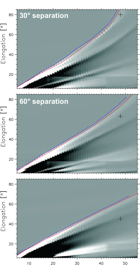
Figure 4.: Jmaps for the three separations with the measured tracks of the ICME front over plotted. The red line is the innermost track and the blue line is the outermost track. The black crosses mark the elongation of the in-situ spacecraft at shock arrival time.fig:jmaptrack

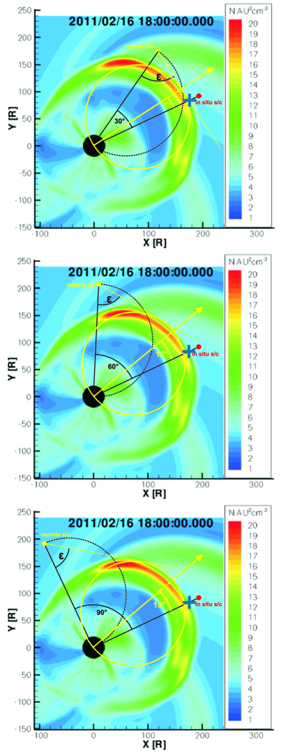
Figure 5.: Top view of the modeled ICME. The denser region (red part) is located at the western flank of the ICME. The spacecraft positions (yellow and red dots) and resulting directions from the CHM method (yellow arrow) for all three separations (top: $30^{\circ}$, middle: $60^{\circ}$, bottom: $90^{\circ}$) are over plotted. The black semicircle is the TS and the yellow dashed line is the tangent to the circle assumed by the Harmonic Mean approximation. The blue cross marks the ICME apex that was measured from top view.fig:topview

The resulting directions obtained for the mean of the innermost and the outermost Jmap tracks are shown in Figure fig:topview. The yellow circle is the assumed circular shape of the HM approximation and the yellow arrow marks the direction of the ICME apex. The dashed semicircle is the TS. For all three separation cases the resulting directions are consistent within a few degrees ($30^{\circ}$ sep: $\phi=$ W7; $60^{\circ}$ sep: $\phi=$ W12; $90^{\circ}$ sep: $\phi=$ W15; true dir.: E0/W0). Because of the corotating interaction region (CIR), heading in front of the ICME, the western flank is denser, which may be the reason for a result toward the western direction. The resulting propagation angles for the innermost tracks are 2 – $4^{\circ}$ larger than the directions calculated from the outermost tracks (see Table tab:direc). To demonstrate how well the CHM method works, we calculate the directions also for the constrained F$\phi$ method using the constraint of the in-situ data point of the arrival time of the ICME (see Rollett et al., 2012). F$\phi$ assumes a single point moving radially away from the Sun and is thus more dependent on the separation of both spacecraft and/or the remote spacecraft to the ICME apex than HM.

Table 3.: Resulting ICME propagation directions for the three separation cases. Constrained Fixed-$\phi$ (CF$\phi$) and constrained Harmonic Mean (CHM) methods are used to calculate the directions for the innermost (inn.) as well as for the outermost (out.) track in the Jmap.tab:direc

	$30^{\circ}$ separation		$60^{\circ}$ separation		$90^{\circ}$ separation
	inn.	out.	inn.	out.	inn.	out.
CHM	W6	W8	W10	W14	W15	W16
CF$\phi$	W13	W17	W22	W28	W32	W25

In Figure fig:dist the converted Jmap measurements (solid lines) are compared to the real ICME apex distance–time profile (dashed line). The top panel shows the $30^{\circ}$ separation case which overestimates the distance especially for the HI1 FoV. The best match of measurements and ICME apex is given for the innermost edge (red line) in the Jmap. The middle panel shows the distance–time profile for $60^{\circ}$ separation revealing that both tracks are in a relatively good agreement with the ICME apex compared to the other separation cases. The bottom panel shows the $90^{\circ}$ separation case. In contrast to the $30^{\circ}$ separation case, the distance is underestimated most of the time. For $60^{\circ}$ and $90^{\circ}$ separation the measurements taken at the outermost edge of the Jmap track reveal the best agreement to the apex measurements.

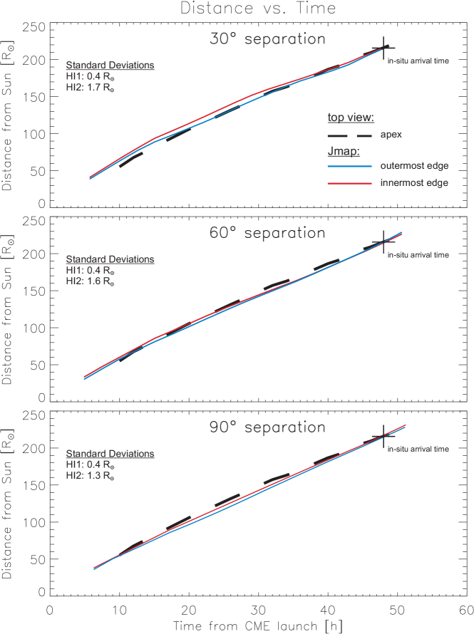
Figure 6.: Distance–time profiles for $30^{\circ},60^{\circ}$, and $90^{\circ}$ separation from the in-situ spacecraft. The dashed line shows the top view measurement of the apex, the solid lines are the conversions from the innermost (red) and the outermost (blue) Jmap measurements., the shaded areas are the error ranges. The crosses indicate the arrival time at the in-situ spacecraft.fig:dist

Figure fig:speed displays the same approach as Figure fig:dist but for the speed–distance profile. The ICME apex enters the HI1 FoV with a speed of $\approx 1100$ km s^-1. It slowly decreases to a mean speed of $\approx 750$ km s^-1. The “true” speed profile of the ICME apex is derived from the top view images. With growing distance from the Sun its standard deviation decreases from 148 km s^-1 to about 62 km s^-1 because of the increasing resolution of the simulation. The speeds derived from the innermost Jmap tracks for all three separation cases show a stronger deceleration than the speed profiles from the outermost edges. The $30^{\circ}$ separation case reveals the best agreement, while the $60^{\circ}$ as well as the $90^{\circ}$ observing angle in the early propagation phase under- and in the late propagation phase overestimate the ICME speed. With growing separation between remote spacecraft and ICME apex the overestimation of the arrival speed increases. While in the $30^{\circ}$ separation case the arrival speed of the outermost edge is quite close to the apex speed, the innermost track underestimates the arrival speed by about 100 km s^-1. From both other viewing angles the arrival speed is overestimated on average by about 75 km s^-1 ($60^{\circ}$ separation) and 125 km s^-1 ($90^{\circ}$ separation), respectively. As well as for the distance–profile, measuring the Jmap track at the innermost edge in the $30^{\circ}$ and $60^{\circ}$ separation cases gives more consistent results compared to the apex.

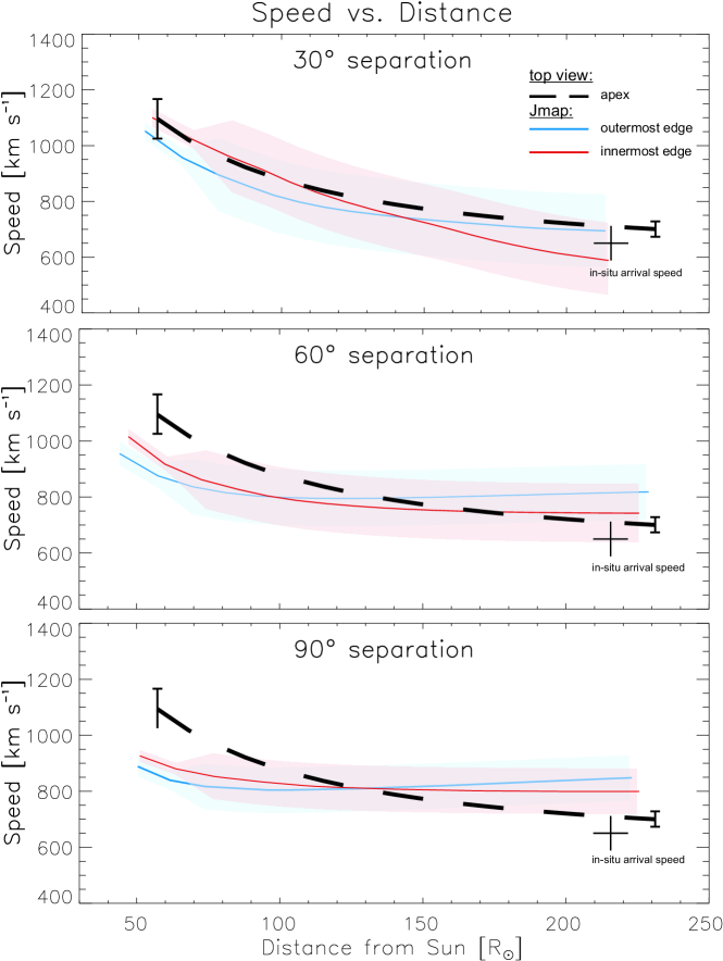
Figure 7.: Speed–distance profiles for $30^{\circ},60^{\circ}$, and $90^{\circ}$ separation from the in-situ spacecraft. The dashed line shows the time derivatives from the top view distance measurement of the apex, the solid lines are the time derivatives from the conversions from the innermost (red) and the outermost (blue) Jmap measurements. The crosses indicate the arrival speed at the in-situ spacecraft.fig:speed

5 Discussion and Conclusions

One aim of this study was to validate the constrained Harmonic Mean method (CHM) introduced in Rollett et al. (2012). This method assumes a spherical ICME front always attached to the Sun and the observer to look along the tangent of the front. The CHM method uses single-spacecraft heliospheric imager (HI) observations and in-situ data at 1 AU. By constraining the kinematics with the in-situ arrival time it is possible to derive the propagation direction for the ICME apex. In addition we can provide distance–time and speed–distance profiles for the entire propagation phase. The second purpose was to provide a reliable error estimate for the kinematics of the ICME when applying the CHM method to Jmap measurements.

In order to test the CHM method we used a numerical simulation of an ICME and analyzed synthetic Jmaps from three different vantage points ($30^{\circ}$, $60^{\circ}$, and $90^{\circ}$ separation of remote spacecraft and in-situ spacecraft). The resulting directions and kinematics for each of the three separation angles were compared to the “true” kinematics of the ICME apex, i.e. free from effects due to Thomson scattering or conversion methods, derived from the top view of the modeled ICME.

The directions obtained seem to be not very sensitive to the separation angle between remote and in-situ spacecraft ($30^{\circ}$ sep: $\phi=$ W7; $60^{\circ}$ sep: $\phi=$ W12; $90^{\circ}$ sep: $\phi=$ W15; true dir.: E0/W0). The density of the ICME is higher in its western flank as a result of a CIR ahead of the ICME. This fact could have influenced our results for the propagation direction and shifted them to a western direction. Another possible reason for that could be that the CHM method assumes a smaller curvature radius of the ICME front than shown by the simulated ICME. It still has to be tested, how the results of the CHM method depend on the ecliptic extend, i.e. the width of the ICME.

Future studies should prove the behavior of the method when ICMEs with different widths are investigated. In Lugaz, Roussev, and Gombosi (2011) the results of the F$\phi$ and HM fitting methods, which assume constant speed, were tested by analyzing a simulated ICME from different viewing angles. Consistent with our study, a stronger dependance of the observing angle for F$\phi$ than for HM was obtained when calculating the propagation direction.

The ICME kinematics were compared to the actual distance–time and speed–distance profiles. The best agreement for the distance is obtained for the $60^{\circ}$ separation case. The $30^{\circ}$ separation case overestimates the distance most of the time while in the $90^{\circ}$ separation case the distance is too small compared to the ICME apex derived from the top view. For the speed–distance profiles the best accordance is revealed by the $30^{\circ}$ separation case. Both other settings first under- and then overestimate the speed. The differences between the true and the calculated arrival speed increases with growing separation ($30^{\circ}$ sep: $\Delta V_{\rm arr}\approx-50$ km s^-1, $60^{\circ}$ sep: $\Delta V_{\rm arr}\approx+75$ km s^-1, $90^{\circ}$ sep: $\Delta V_{\rm arr}\approx+125$ km s^-1). In general, conversion and fitting methods making special geometrical assumptions on the shape of the ICME front, e.g. F$\phi$, HM or SSE methods, overestimate the arrival speed with increasing observation angle.

The error estimation was done by taking into account two different error sources. The intensity area in the Jmap, where the apparent ICME front could be measured, varies between $\pm 0.3^{\circ}$ (HI1) and $\pm 1.35^{\circ}$ elongation (HI2). This should reflect the range of tracks if more than one person measures the front. This is in agreement with the results found by Williams et al. (2009) who quantified the elongation range of chosen tracks measured within a Jmap with less than $\pm 1^{\circ}$ for HI1 and $\pm 2^{\circ}$ for HI2. We find that in general, measuring the Jmap track at the innermost edge gives more consistent results compared to the apex kinematics. The second error is due to the visual measuring of the front and is obtained by calculating the standard deviations out of five measurements taken that lie in a range of $\pm 0.1^{\circ}$ (HI1) and $\pm 0.4^{\circ}$ (HI2). The errors within the speed-profiles lie in a range of 27–34 km s^-1 (HI) and 81–128 km s^-1 (HI2).

The two STEREO spacecraft already are on the backside of the Sun, and thus a forecast for Earth directed ICMEs using the heliospheric imagers is no longer possible. To improve existing space weather forecast an L₄/L₅ mission carrying heliospheric imagers is a valuable option. The side view of the entire distance from the Sun up to 1 AU is a big advantage upon coronagraphic observations from Earth view.

Acknowledgements

This work has received funding from the European Commission FP7 Project n^∘ 263252 [COMESEP]. M. T. acknowledges the Austrian Science Fund (FWF): V195-N16. This research was supported by a Marie Curie International Outgoing Fellowship within the 7th European Community Framework Programme. N. L. was supported by NSF AGS1239704 and NASA NNX12AB28G. Simulation results were obtained using the Space Weather Modeling Framework, developed by the Center for Space Environment Modeling, at the University of Michigan with funding support from NASA ESS, NASA ESTO-CT, NSF KDI, and DoD MURI. We thank the STEREO SECCHI/IMPACT/PLASTIC teams for their open data policy.

References

- Arge and Pizzo (2000) Arge, C.N., Pizzo, V.J.: 2000, Improvement in the prediction of solar wind conditions using near-real time solar magnetic field updates. J. Geophys. Res. 105, 10465 – 10480. doi:10.1029/1999JA900262.
- Bein et al. (2011) Bein, B.M., Berkebile-Stoiser, S., Veronig, A.M., Temmer, M., Muhr, N., Kienreich, I., Utz, D., Vršnak, B.: 2011, Impulsive Acceleration of Coronal Mass Ejections. I. Statistics and Coronal Mass Ejection Source Region Characteristics. ApJ 738, 191. doi:10.1088/0004-637X/738/2/191.
- Billings (1966) Billings, D.E.: 1966, A guide to the solar corona.
- Brueckner et al. (1995) Brueckner, G.E., Howard, R.A., Koomen, M.J., Korendyke, C.M., Michels, D.J., Moses, J.D., Socker, D.G., Dere, K.P., Lamy, P.L., Llebaria, A., Bout, M.V., Schwenn, R., Simnett, G.M., Bedford, D.K., Eyles, C.J.: 1995, The Large Angle Spectroscopic Coronagraph (LASCO). Sol. Phys. 162, 357 – 402. doi:10.1007/BF00733434.
- Burlaga, Plunkett, and St. Cyr (2002) Burlaga, L.F., Plunkett, S.P., St. Cyr, O.C.: 2002, Successive CMEs and complex ejecta. Journal of Geophysical Research (Space Physics) 107, 1266. doi:10.1029/2001JA000255.
- Cohen et al. (2007) Cohen, O., Sokolov, I.V., Roussev, I.I., Arge, C.N., Manchester, W.B., Gombosi, T.I., Frazin, R.A., Park, H., Butala, M.D., Kamalabadi, F., Velli, M.: 2007, A Semiempirical Magnetohydrodynamical Model of the Solar Wind. ApJ 654, L163. doi:10.1086/511154.
- Davies et al. (2009) Davies, J.A., Harrison, R.A., Rouillard, A.P., Sheeley, N.R., Perry, C.H., Bewsher, D., Davis, C.J., Eyles, C.J., Crothers, S.R., Brown, D.S.: 2009, A synoptic view of solar transient evolution in the inner heliosphere using the Heliospheric Imagers on STEREO. Geophys. Res. Lett. 36, L02102. doi:10.1029/2008GL036182.
- Davies et al. (2012) Davies, J.A., Harrison, R.A., Perry, C.H., Möstl, C., Lugaz, N., Rollett, T., Davis, C.J., Crothers, S.R., Temmer, M., Eyles, C.J., Savani, N.P.: 2012, A Self-similar Expansion Model for Use in Solar Wind Transient Propagation Studies. ApJ 750, 23. doi:10.1088/0004-637X/750/1/23.
- Eyles et al. (2009) Eyles, C.J., Harrison, R.A., Davis, C.J., Waltham, N.R., Shaughnessy, B.M., Mapson-Menard, H.C.A., Bewsher, D., Crothers, S.R., Davies, J.A., Simnett, G.M., Howard, R.A., Moses, J.D., Newmark, J.S., Socker, D.G., Halain, J.-P., Defise, J.-M., Mazy, E., Rochus, P.: 2009, The Heliospheric Imagers Onboard the STEREO Mission. Sol. Phys. 254, 387 – 445. doi:10.1007/s11207-008-9299-0.
- Gallagher, Lawrence, and Dennis (2003) Gallagher, P.T., Lawrence, G.R., Dennis, B.R.: 2003, Rapid Acceleration of a Coronal Mass Ejection in the Low Corona and Implications for Propagation. ApJ 588, L53. doi:10.1086/375504.
- Gopalswamy et al. (2001) Gopalswamy, N., Yashiro, S., Kaiser, M.L., Howard, R.A., Bougeret, J.-L.: 2001, Radio Signatures of Coronal Mass Ejection Interaction: Coronal Mass Ejection Cannibalism? ApJ 548, L91. doi:10.1086/318939.
- Gopalswamy et al. (2011) Gopalswamy, N., Davila, J.M., St. Cyr, O.C., Sittler, E.C., Auchère, F., Duvall, T.L., Hoeksema, J.T., Maksimovic, M., MacDowall, R.J., Szabo, A., Collier, M.R.: 2011, Earth-Affecting Solar Causes Observatory (EASCO): A potential International Living with a Star Mission from Sun-Earth L5. Journal of Atmospheric and Solar-Terrestrial Physics 73, 658 – 663. doi:10.1016/j.jastp.2011.01.013.
- Harrison et al. (2009) Harrison, R.A., Davies, J.A., Rouillard, A.P., Davis, C.J., Eyles, C.J., Bewsher, D., Crothers, S.R., Howard, R.A., Sheeley, N.R., Vourlidas, A., Webb, D.F., Brown, D.S., Dorrian, G.D.: 2009, Two Years of the STEREO Heliospheric Imagers. Invited Review. Sol. Phys. 256, 219 – 237. doi:10.1007/s11207-009-9352-7.
- Howard et al. (2008) Howard, R.A., Moses, J.D., Vourlidas, A., Newmark, J.S., Socker, D.G., Plunkett, S.P., Korendyke, C.M., Cook, J.W., Hurley, A., Davila, J.M., Thompson, W.T., St Cyr, O.C., Mentzell, E., Mehalick, K., Lemen, J.R., Wuelser, J.P., Duncan, D.W., Tarbell, T.D., Wolfson, C.J., Moore, A., Harrison, R.A., Waltham, N.R., Lang, J., Davis, C.J., Eyles, C.J., Mapson-Menard, H., Simnett, G.M., Halain, J.P., Defise, J.M., Mazy, E., Rochus, P., Mercier, R., Ravet, M.F., Delmotte, F., Auchere, F., Delaboudiniere, J.P., Bothmer, V., Deutsch, W., Wang, D., Rich, N., Cooper, S., Stephens, V., Maahs, G., Baugh, R., McMullin, D., Carter, T.: 2008, Sun Earth Connection Coronal and Heliospheric Investigation (SECCHI). Space Sci. Rev. 136, 67 – 115. doi:10.1007/s11214-008-9341-4.
- Howard and DeForest (2012) Howard, T.A., DeForest, C.E.: 2012, The Thomson Surface. I. Reality and Myth. ApJ 752, 130. doi:10.1088/0004-637X/752/2/130.
- Howard and Tappin (2009) Howard, T.A., Tappin, S.J.: 2009, Interplanetary Coronal Mass Ejections Observed in the Heliosphere: 1. Review of Theory. Space Sci. Rev. 147, 31 – 54. doi:10.1007/s11214-009-9542-5.
- Hundhausen (1993) Hundhausen, A.J.: 1993, Sizes and locations of coronal mass ejections - SMM observations from 1980 and 1984-1989. J. Geophys. Res. 981, 13177. doi:10.1029/93JA00157.
- Kahler and Webb (2007) Kahler, S.W., Webb, D.F.: 2007, V arc interplanetary coronal mass ejections observed with the Solar Mass Ejection Imager. J. Geophys. Res. 112, 9103. doi:10.1029/2007JA012358.
- Kaiser et al. (2008) Kaiser, M.L., Kucera, T.A., Davila, J.M., St. Cyr, O.C., Guhathakurta, M., Christian, E.: 2008, The STEREO Mission: An Introduction. Space Sci. Rev. 136, 5 – 16. doi:10.1007/s11214-007-9277-0.
- Liu et al. (2010) Liu, Y., Davies, J.A., Luhmann, J.G., Vourlidas, A., Bale, S.D., Lin, R.P.: 2010, Geometric Triangulation of Imaging Observations to Track Coronal Mass Ejections Continuously Out to 1 AU. ApJ 710, L82. doi:10.1088/2041-8205/710/1/L82.
- Lugaz (2010) Lugaz, N.: 2010, Accuracy and Limitations of Fitting and Stereoscopic Methods to Determine the Direction of Coronal Mass Ejections from Heliospheric Imagers Observations. Sol. Phys. 267, 411 – 429. doi:10.1007/s11207-010-9654-9.
- Lugaz, Roussev, and Gombosi (2011) Lugaz, N., Roussev, I.I., Gombosi, T.I.: 2011, Determining CME parameters by fitting heliospheric observations: Numerical investigation of the accuracy of the methods. Adv. Space Res. 48, 292 – 299. doi:10.1016/j.asr.2011.03.015.
- Lugaz, Vourlidas, and Roussev (2009a) Lugaz, N., Vourlidas, A., Roussev, I.I.: 2009a, Deriving the radial distances of wide coronal mass ejections from elongation measurements in the heliosphere - application to CME-CME interaction. Annales Geophysicae 27, 3479 – 3488.
- Lugaz et al. (2009b) Lugaz, N., Vourlidas, A., Roussev, I.I., Morgan, H.: 2009b, Solar-Terrestrial Simulation in the STEREO Era: The 24–25 January 2007 Eruptions. Sol. Phys. 256, 269 – 284. doi:10.1007/s11207-009-9339-4.
- Luhmann et al. (2008) Luhmann, J.G., Curtis, D.W., Schroeder, P., McCauley, J., Lin, R.P., Larson, D.E., Bale, S.D., Sauvaud, J.-A., Aoustin, C., Mewaldt, R.A., Cummings, A.C., Stone, E.C., Davis, A.J., Cook, W.R., Kecman, B., Wiedenbeck, M.E., von Rosenvinge, T., Acuna, M.H., Reichenthal, L.S., Shuman, S., Wortman, K.A., Reames, D.V., Mueller-Mellin, R., Kunow, H., Mason, G.M., Walpole, P., Korth, A., Sanderson, T.R., Russell, C.T., Gosling, J.T.: 2008, STEREO IMPACT Investigation Goals, Measurements, and Data Products Overview. Space Sci. Rev. 136, 117 – 184. doi:10.1007/s11214-007-9170-x.
- Möstl and Davies (2012) Möstl, C., Davies, J.A.: 2012, Speeds and Arrival Times of Solar Transients Approximated by Self-similar Expanding Circular Fronts. Sol. Phys., 77. doi:10.1007/s11207-012-9978-8.
- Möstl et al. (2009a) Möstl, C., Farrugia, C.J., Temmer, M., Miklenic, C., Veronig, A.M., Galvin, A.B., Leitner, M., Biernat, H.K.: 2009a, Linking Remote Imagery of a Coronal Mass Ejection to Its In Situ Signatures at 1 AU. ApJ 705, L180. doi:10.1088/0004-637X/705/2/L180.
- Möstl et al. (2009b) Möstl, C., Farrugia, C.J., Miklenic, C., Temmer, M., Galvin, A.B., Luhmann, J.G., Kilpua, E.K.J., Leitner, M., Nieves-Chinchilla, T., Veronig, A., Biernat, H.K.: 2009b, Multispacecraft recovery of a magnetic cloud and its origin from magnetic reconnection on the Sun. J. Geophys. Res. 114, 4102. doi:10.1029/2008JA013657.
- Möstl et al. (2010) Möstl, C., Temmer, M., Rollett, T., Farrugia, C.J., Liu, Y., Veronig, A.M., Leitner, M., Galvin, A.B., Biernat, H.K.: 2010, STEREO and Wind observations of a fast ICME flank triggering a prolonged geomagnetic storm on 5-7 April 2010. Geophys. Res. Lett. 372, L24103. doi:10.1029/2010GL045175.
- Möstl et al. (2011) Möstl, C., Rollett, T., Lugaz, N., Farrugia, C.J., Davies, J.A., Temmer, M., Veronig, A.M., Harrison, R.A., Crothers, S., Luhmann, J.G., Galvin, A.B., Zhang, T.L., Baumjohann, W., Biernat, H.K.: 2011, Arrival Time Calculation for Interplanetary Coronal Mass Ejections with Circular Fronts and Application to STEREO Observations of the 2009 February 13 Eruption. ApJ 741, 34. doi:10.1088/0004-637X/741/1/34.
- Ogilvie et al. (1995) Ogilvie, K.W., Chornay, D.J., Fritzenreiter, R.J., Hunsaker, F., Keller, J., Lobell, J., Miller, G., Scudder, J.D., Sittler, E.C. Jr., Torbert, R.B., Bodet, D., Needell, G., Lazarus, A.J., Steinberg, J.T., Tappan, J.H., Mavretic, A., Gergin, E.: 1995, SWE, A Comprehensive Plasma Instrument for the Wind Spacecraft. Space Sci. Rev. 71, 55 – 77.
- Rollett et al. (2012) Rollett, T., Möstl, C., Temmer, M., Veronig, A.M., Farrugia, C.J., Biernat, H.K.: 2012, Constraining the Kinematics of Coronal Mass Ejections in the Inner Heliosphere with In-Situ Signatures. Sol. Phys. 276, 293 – 314. doi:10.1007/s11207-011-9897-0.
- Rouillard (2011) Rouillard, A.P.: 2011, Relating white light and in situ observations of coronal mass ejections: A review. Journal of Atmospheric and Solar-Terrestrial Physics 73, 1201 – 1213. doi:10.1016/j.jastp.2010.08.015.
- Rouillard et al. (2008) Rouillard, A.P., Davies, J.A., Forsyth, R.J., Rees, A., Davis, C.J., Harrison, R.A., Lockwood, M., Bewsher, D., Crothers, S.R., Eyles, C.J., Hapgood, M., Perry, C.H.: 2008, First imaging of corotating interaction regions using the STEREO spacecraft. Geophys. Res. Lett. 35, 10110. doi:10.1029/2008GL033767.
- Sheeley et al. (2008) Sheeley, N.R. Jr., Herbst, A.D., Palatchi, C.A., Wang, Y.-M., Howard, R.A., Moses, J.D., Vourlidas, A., Newmark, J.S., Socker, D.G., Plunkett, S.P., Korendyke, C.M., Burlaga, L.F., Davila, J.M., Thompson, W.T., St Cyr, O.C., Harrison, R.A., Davis, C.J., Eyles, C.J., Halain, J.P., Wang, D., Rich, N.B., Battams, K., Esfandiari, E., Stenborg, G.: 2008, Heliospheric Images of the Solar Wind at Earth. ApJ 675, 853 – 862. doi:10.1086/526422.
- Sheeley et al. (1999) Sheeley, N.R., Walters, J.H., Wang, Y.-M., Howard, R.A.: 1999, Continuous tracking of coronal outflows: Two kinds of coronal mass ejections. J. Geophys. Res. 104, 24739 – 24768. doi:10.1029/1999JA900308.
- Stone et al. (1998) Stone, E.C., Frandsen, A.M., Mewaldt, R.A., Christian, E.R., Margolies, D., Ormes, J.F., Snow, F.: 1998, The Advanced Composition Explorer. Space Sci. Rev. 86, 1 – 22. doi:10.1023/A:1005082526237.
- Temmer et al. (2011) Temmer, M., Rollett, T., Möstl, C., Veronig, A.M., Vršnak, B., Odstrčil, D.: 2011, Influence of the Ambient Solar Wind Flow on the Propagation Behavior of Interplanetary Coronal Mass Ejections. ApJ 743, 101. doi:10.1088/0004-637X/743/2/101.
- Temmer et al. (2012) Temmer, M., Vršnak, B., Rollett, T., Bein, B., de Koning, C.A., Liu, Y., Bosman, E., Davies, J.A., Möstl, C., Žic, T., Veronig, A.M., Bothmer, V., Harrison, R., Nitta, N., Bisi, M., Flor, O., Eastwood, J., Odstrcil, D., Forsyth, R.: 2012, Characteristics of Kinematics of a Coronal Mass Ejection during the 2010 August 1 CME-CME Interaction Event. ApJ 749, 57. doi:10.1088/0004-637X/749/1/57.
- Tóth et al. (2005) Tóth, G., Sokolov, I.V., Gombosi, T.I., Chesney, D.R., Clauer, C.R., De Zeeuw, D.L., Hansen, K.C., Kane, K.J., Manchester, W.B., Oehmke, R.C., Powell, K.G., Ridley, A.J., Roussev, I.I., Stout, Q.F., Volberg, O., Wolf, R.A., Sazykin, S., Chan, A., Yu, B., Kóta, J.: 2005, Space Weather Modeling Framework: A new tool for the space science community. Journal of Geophysical Research (Space Physics) 110, 12226. doi:10.1029/2005JA011126.
- Vourlidas and Howard (2006) Vourlidas, A., Howard, R.A.: 2006, The Proper Treatment of Coronal Mass Ejection Brightness: A New Methodology and Implications for Observations. ApJ 642, 1216 – 1221. doi:10.1086/501122.
- Vršnak et al. (2012) Vršnak, B., Žic, T., Vrbanec, D., Temmer, M., Rollett, T., Möstl, C., Veronig, A., Čalogović, J., Dumbović, M., Lulić, S., Moon, Y.-J., Shanmugaraju, A.: 2012, Propagation of Interplanetary Coronal Mass Ejections: The Drag-Based Model. Sol. Phys., 124. doi:10.1007/s11207-012-0035-4.
- Wang and Sheeley (1990) Wang, Y.-M., Sheeley, N.R. Jr.: 1990, Solar wind speed and coronal flux-tube expansion. ApJ 355, 726 – 732. doi:10.1086/168805.
- Williams et al. (2009) Williams, A.O., Davies, J.A., Milan, S.E., Rouillard, A.P., Davis, C.J., Perry, C.H., Harrison, R.A.: 2009, Deriving solar transient characteristics from single spacecraft STEREO/HI elongation variations: a theoretical assessment of the technique. Annales Geophysicae 27, 4359 – 4368. doi:10.5194/angeo-27-4359-2009.
- Zhang et al. (2001) Zhang, J., Dere, K.P., Howard, R.A., Kundu, M.R., White, S.M.: 2001, On the Temporal Relationship between Coronal Mass Ejections and Flares. ApJ 559, 452 – 462. doi:10.1086/322405.