An Impossibility Result for High Dimensional Supervised Learning

Abstract

We study high-dimensional asymptotic performance limits of binary supervised classification problems where the class conditional densities are Gaussian with unknown means and covariances and the number of signal dimensions scales faster than the number of labeled training samples. We show that the Bayes error, namely the minimum attainable error probability with complete distributional knowledge and equally likely classes, can be arbitrarily close to zero and yet the limiting minimax error probability of every supervised learning algorithm is no better than a random coin toss. In contrast to related studies where the classification difficulty (Bayes error) is made to vanish, we hold it constant when taking high-dimensional limits. In contrast to VC-dimension based minimax lower bounds that consider the worst case error probability over all distributions that have a fixed Bayes error, our worst case is over the family of Gaussian distributions with constant Bayes error. We also show that a nontrivial asymptotic minimax error probability can only be attained for parametric subsets of zero measure (in a suitable measure space). These results expose the fundamental importance of prior knowledge and suggest that unless we impose strong structural constraints, such as sparsity, on the parametric space, supervised learning may be ineffective in high dimensional small sample settings.

I Introduction

In a number of applications ranging from medical imaging to economics, one encounters inference problems that suffer from the “curse of dimensionality”, namely the situation where the observed signals are high-dimensional and we lack sufficient labeled training samples from which to accurately learn models and make reliable decisions. This may be true even when the underlying decision problem becomes “easy” with perfect knowledge of models or latent variables. For example, in detecting the presence or absence of stroke, high-dimensional tomographic X-ray projections are measured, though a stroke may affect only tissue properties in a localized spatial region and may be easily detectable if one knew where to look. Labeled training samples are typically limited in this context due to the high cost of engaging domain experts. Research in recent years has therefore focused on leveraging prior knowledge in the form of sparsity or other latent low-dimensional structure to improve decision making.

Our aim in this work is to expose certain fundamental limitations of supervised learning in high dimensional small sample settings and highlight the fundamental necessity of strong structural constraints (prior knowledge), such as sparsity, for attaining nontrivial asymptotic error rates. Towards this end we study the high-dimensional asymptotic performance limit of binary supervised classification where the class conditional densities are Gaussian with unknown means and covariances. If $d$ and $n$ respectively denote the number of signal dimensions and the number of labeled training samples, our focus is on the “big $d$ small $n$” asymptotic regime where $n/d\rightarrow 0$ as $d\rightarrow\infty$. In previous related work, either $n/d\rightarrow c>0$ as $d\rightarrow\infty$ or the classification difficulty (Bayes error) converges to zero as $d\rightarrow\infty$ [1, 2], or the focus was on special families of learning rules such as Naive-Bayes, banded covariance structure [3], and plug-in rules [4, 5]. In contrast, we hold the Bayes error constant when taking high-dimensional limits.

We establish two key results in this paper: 1) An impossibility result: When the number of signal dimensions scales faster than the number of labeled samples at constant classification difficulty, the asymptotic minimax classification error probability of any supervised classification algorithm cannot converge to anything less than half. 2) Necessity of “structure” in parameter set: Nontrivial asymptotic minimax error probability is attainable only for parametric subsets of zero Haar measure.

II Related results from VC Theory

There are several well known probabilistic lower bounds for the error probability in the distribution-free setting of learning [6]. These bounds are typically based on the VC dimension $V$ of a set of classifiers containing the optimal Bayes rule. For the case when the Bayes error $P^{*}_{e}$ is zero, it is known that if $n<(V-1)/(32\epsilon)$, then for any supervised classifier $g_{n}$ and all $\epsilon\leq 1/8$ and $\delta\leq 0.01$, $\sup_{p_{X,Y}:P^{*}_{e}=0}\Pr(L_{g_{n}}\geq\epsilon)\geq\delta$ [7], where $p_{X,Y}$ is the joint distribution of data points and their labels, $L_{g_{n}}=\Pr(g_{n}(X)\neq Y|X_{1},Y_{1},\ldots,X_{n},Y_{n})$, and $\{(X_{1},Y_{1}),\ldots,(X_{n},Y_{n})\}$ is the training set. This bound implies that if $n$ is small compared to $V$, then there exist distributions for which, with probability of at least $0.01$, the conditional Bayes error of every classifier is larger than $1/8$. For the case when $P^{*}_{e}=c\neq 0$, it is known that if $n<V/(320\epsilon)$ then for all supervised learning rules $g_{n}$, and all $\epsilon,\delta\in(0,1/64)$, $\sup_{p_{X,Y}:P^{*}_{e}=c}\Pr(L_{g_{n}}-c\geq\epsilon)\geq\delta$. For linear classifiers in $\mathbb{R}^{d}$, $V=(d+1)$ and the mentioned bounds prove the impossibility of learnability in the distribution-free high dimensional setting. However, these bounds are known to be pessimistic as they are proved by constructing pathological adversarial distributions $p_{X|Y}$ whose support is concentrated on $V$ points in order to make the error of any learning rule in the hypothesis space larger than $\epsilon$ with probability of at least $\delta$. It has been suggested that these bounds do not hold for some practical choices of $p_{X,Y}$ [8].

There also exist impossibility results for the fixed distribution setting [9] where a fixed and known distribution $p_{X}$ is assumed and classifiers are assumed to belong to a specific set $\mathcal{C}$. For $\Pr(L_{g_{n}}\leq\epsilon)\geq 1-\delta$ it is necessary that $n\geq\log((1-\delta)n_{c})$ where $n_{c}$ is the $\epsilon$ covering number of $\mathcal{C}$ with respect to $p_{X}$ [9].

The learning scenario discussed in this paper differs from both these settings. We consider $p_{X|Y,\theta}$ to be a Gaussian distribution with an unknown set of parameters $\theta$. Hence, unlike the second setting, $p_{X}$ is not a fixed distribution, but belongs to a family of Gaussian distributions parameterized by different choices of $\theta$. However, this family is much more restricted than the set of all distributions, which is assumed in the distribution-free setting. In addition, we establish a stronger notion of impossibility that corresponds to taking $\epsilon=\frac{1}{2}$ and $\delta=1$ asymptotically, i.e., the worst-case error probability within the family is not less than half asymptotically. It should also be noted that our notion of impossibility is not available in the distribution-free setting, and additional effort is required to establish it in the fixed-distribution setting.

III Problem Formulation

Binary classification with Gaussian class conditional densities: Let $X\in\mathbb{R}^{d}$ denote the observed signal (data), $Y\in\{-1,+1\}$ the latent binary class label with $p_{Y}(+1)=p_{Y}(-1)=1/2$, and $p_{X|Y,\theta}(x|y,\theta)=\mathcal{N}(\mu_{y},\Sigma)(x)$, where $\mu_{+1},\mu_{-1}\in\mathbb{R}^{d}$, $\mu_{+1}\neq\mu_{-1}$ are mean vectors for classes $+1$ and $-1$ respectively, $\Sigma$ is a covariance matrix common to both classes, and $\theta:=(\mu_{+1},\mu_{-1},\Sigma)$ denotes the tuple of parameters. Thus $(X,Y)|\theta\sim p_{X|Y,\theta}(x|y,\theta)p_{Y}(y)$. The minimum probability of error classification rule, henceforth referred to as the optimum rule, is the maximum aposteriori probability (MAP) rule and is given by

$$\begin{split}\widehat{y}^{*}(x)&=\operatorname*{arg\,max}_{y\in\{-1,+1\}}p_{Y|X,\theta}(y|x,\theta)\\ &=\operatorname{sign}\left(\Delta^{T}\Sigma^{+}(x-\mu)\right)\end{split}$$ (1)

where $\mu:=\frac{1}{2}(\mu_{+1}+\mu_{-1})$, $\Delta:=\mu_{+1}-\mu_{-1}$, and $\Sigma^{+}$ is the pseudoinverse of $\Sigma$. The error probability of the optimum rule (Bayes error) is given by

$$P_{e}^{*}=Q\left(\frac{1}{2}\left\|\left(\Sigma^{+}\right)^{\frac{1}{2}}\left(\mu_{+1}-\mu_{-1}\right)\right\|\right)=:Q(\alpha/2)$$ (2)

where $Q(t):=\int_{t}^{\infty}\frac{1}{\sqrt{2\pi}}\exp\{-\frac{1}{2}t^{2}\}dt$, $\alpha=\|(\Sigma^{+})^{\frac{1}{2}}(\mu_{+1}-\mu_{-1})\|$, and the minimum attainable error probability with complete distributional knowledge and equally likely classes, i.e., the “classification difficulty”, is given by $Q(\alpha/2)$. We will assume that $\alpha>0$ so that the Bayes error is nontrivial, i.e, strictly less than $1/2$.

Supervised classification rules: Let $\mathcal{T}_{n}:=\{(X_{i},Y_{i}),i=1,\ldots,n\}$ be a set of $n$ labeled training samples that are independent and identically distributed (iid) according to $p_{X|Y,\theta}\cdot p_{Y}$ where $\theta$ belongs to a known set of feasible parameters $\Theta$. Let $X_{0}$ be a test sample (independent of $\mathcal{T}_{n}$) whose true class label $Y_{0}$ is unobservable and needs to be estimated. A supervised classification rule is a measurable mapping

$$\widehat{y}_{n,d}:\mathbb{R}^{d}\times\mathcal{T}_{n}\rightarrow\{-1,+1\}$$

from the test data space to the set of class labels constructed using an algorithm that has access to the set of training samples $\mathcal{T}_{n}$ and knowledge of the form of $p_{X,Y|\theta}(x,y|\theta)$ and $\Theta$ but no direct knowledge of $\theta$ itself.

Constant difficulty parameter sets: We are interested in taking constant-difficulty high-dimensional limits. To this end we define $\Theta_{0}(\alpha)$ to be the set of all $\theta$ values for which the Bayes error is equal to $Q(\alpha/2)$ (see (2)):

$$\Theta_{0}(\alpha):=\left\{\left(\mu_{+1},\mu_{-1},\Sigma\right):\left\|\ \left(\Sigma^{+}\right)^{\frac{1}{2}}\left(\mu_{+1}-\mu_{-1}\right)\right\|=\alpha\right\}.$$

A canonical subset of $\Theta_{0}$ of particular interest is one in which the covariance is spherical and the means are constrained to be on opposites ends of a $d$-dimensional sphere:

$$\Theta_{\text{Sphere}}(\alpha):=\left\{\left({\mathbf{h}},-{\mathbf{h}},\beta^{2}{\mathbf{I}}\right):\lVert{\mathbf{h}}\rVert=1,\beta=2/\alpha\right\}.$$

Clearly, $\Theta_{\text{Sphere}}(\alpha)\subseteq\Theta_{0}(\alpha)$. This special parametric set corresponds to the scenario in which $X$ can be represented as $X=Y{\mathbf{h}}+Z$ where $Z$ is white Gaussian noise that is independent of $Y$.

Error probabilities: Let

$$P_{e|\theta}(\widehat{y}_{n,d}):=\Pr\left(\widehat{y}_{n,d}(X_{0})\neq Y_{0}\right)$$

denote the expected error probability of the classifier $\widehat{y}_{n,d}$ averaged across training samples $\mathcal{T}_{n}$ for some parameter $\theta$ and let

$$P_{e}(n,d,\Theta,\widehat{y}_{n,d}):=\sup_{\theta\in\Theta}P_{e|\theta}(\widehat{y}_{n,d})$$

be the maximum expected error probability of the classifier $\widehat{y}_{n,d}$ over the parameter set $\Theta$ which depends on the number of labeled training samples $n$ and the number of signal dimensions $d$.

Goal: We aim to gain an understanding of how $P_{e}(n,d,\Theta,\widehat{y}_{n,d})$ behaves in the constant-difficulty high dimensional setting where $d,n\rightarrow\infty$, $n/d,n/\text{rank}(\Sigma^{+})\rightarrow 0$, and $\Theta\subseteq\Theta_{0}(\alpha)$ is a sequence of constant-difficulty parameter sets.

IV Main Results

Theorem 1.

For any sequence of classifiers $\widehat{y}_{n,d}$, we have

$$\liminf\limits_{(d,n/d)\rightarrow(\infty,0)}P_{e}(n,d,\Theta_{\text{Sphere}},\widehat{y}_{n,d})\geq\frac{1}{2}$$

Corollary 1.

For any sequence of parameter sets $\Theta$ with $\Theta_{\text{Sphere}}\subseteq\Theta$, and any sequence of classifiers $\widehat{y}_{n,d}$, we have

$$\liminf\limits_{(d,n/d)\rightarrow(\infty,0)}P_{e}(n,d,\Theta,\widehat{y}_{n,d})\geq\frac{1}{2}$$

Corollary 2.

Let $\Theta_{\text{subset}}:=\{({\mathbf{h}},-{\mathbf{h}},\beta^{2}{\mathbf{I}})\in\Theta_{\text{Sphere}},\mathbf{h}\in\mathcal{H}\subseteq\mathcal{S}^{d-1}\}$ where $\mathcal{S}^{d-1}$ is the unit $(d-1)$-sphere in $\mathbb{R}^{d}$. Let $\operatorname{vol}({\mathcal{H}})\triangleq\Pr_{H\sim U(\mathcal{S}^{d-1})}(H\in\mathcal{H})$, where $U(\mathcal{S}^{d-1})$ denotes the uniform distribution over $\mathcal{S}^{d-1}$. If for a sequence of classifiers $\widehat{y}_{n,d}$,

$$\limsup\limits_{(d,n/d)\rightarrow(\infty,0)}P_{e}(n,d,\Theta_{\text{Sphere}},\widehat{y}_{n,d})=\frac{1}{2}$$

and

$$\lim_{d\rightarrow\infty}\operatorname{vol}({\mathcal{H}})>0$$

then

$$\limsup\limits_{(d,n/d)\rightarrow(\infty,0)}P_{e}(n,d,\Theta_{\text{subset}},\widehat{y}_{n,d})\geq\frac{1}{2}.$$

The proofs of the theorem and the two corollaries are presented in Section VI.

V Discussion

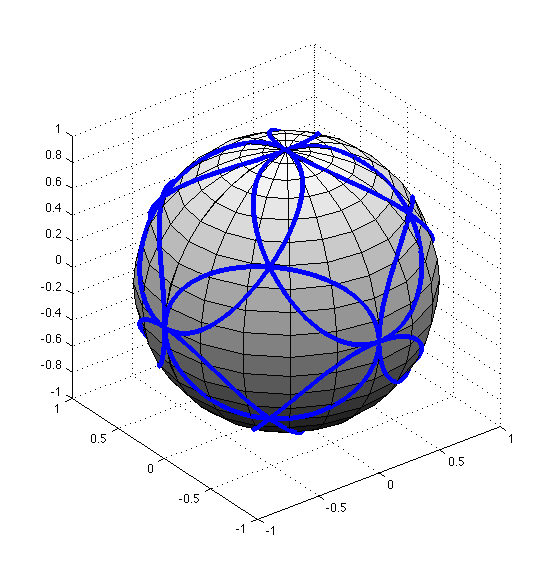
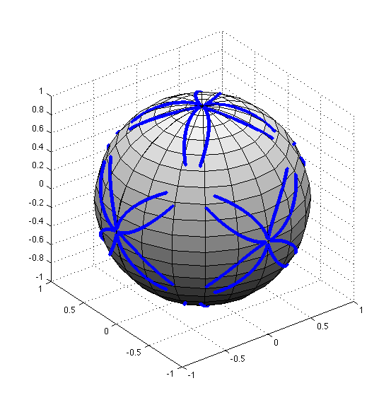
Figure 1: Exponential sparsity class $\mathcal{H}_{exp}$ (solid curves, top figure) and polynomial sparsity class $\mathcal{H}_{poly}$ (solid curves, bottom figure) for $d=3$.

Theorem 1 informs us that even in the “easier” scenario where the covariance is spherical and perfectly known, the worst case classification performance of any sequence of supervised classifiers is asymptotically no better than the classifier which flips an unbiased coin to make decisions. It is interesting to note that this conclusion holds for any arbitrarily small positive Bays error $Q(\alpha/2)$.

An immediate corollary of this theorem is the impossibility of attaining less than half asymptotic error probability for larger parametric sets, specifically parameter sets that contain $\Theta_{\text{Sphere}}$ such as $\Theta_{0}$. These parameter sets contain more unknowns (degrees of freedom), e.g., the covariance, but have the same classification difficulty $Q(\alpha/2)$.

These results are consistent with previous results concerning the asymptotic behavior of the so-called plug-in family of classifiers where Maximum Likelihood (ML) estimates of parameters are plugged into the MAP rule given in (1)):

• Plug-in classification for $\Theta_{0}$: In [5] it was shown that for plug-in classifiers that use ML estimates of the means and covariance, the performance is asymptotically no better than half.

• Sensing-aware classification: Here it is assumed that data is generated according to $X={\mathbf{h}}W+Z$, where ${\mathbf{h}}$ is the “sensing subspace”, $W$ is a class-dependent scalar latent variable and $Z$ is white Gaussian noise independent of the class labels and latent variables. Assuming Gaussian class conditional densities for $W$, the class conditional density of $X$ would be Gaussian with covariance $\gamma^{2}{\mathbf{h}}{\mathbf{h}}^{\operatorname{\top}}+\beta^{2}{\mathbf{I}}$. Also the mean of $X$ would be in the same direction ${\mathbf{h}}$ for the two classes. In [5] it was shown that the asymptotic probability of error of the ML projection classifier which is based on projecting data along the ML estimate of ${\mathbf{h}}$ is also no better than half. This can be seen as a special case of the Corollary 1, by considering ${\Theta_{\text{Sensing Aware}}}\supseteq\Theta_{\text{Sphere}}$ where

  $${\Theta_{\text{Sensing Aware}}}(\alpha):=\big{\{}\left(m_{1}{\mathbf{h}},m_{2}{\mathbf{h}},\gamma^{2}{\mathbf{h}}{\mathbf{h}}^{\operatorname{\top}}+\beta^{2}{\mathbf{I}}\right):\\ \|{\mathbf{h}}\|=1,\gamma\geq 0,\beta>0,|m_{1}-m_{2}|=\alpha\sqrt{\gamma^{2}+\beta^{2}}\big{\}}.$$

Another important consequence of the Theorem 1 is Corollary 2. This result can be interpreted as implying that nontrivial asymptotic minimax error probability is attainable only for parametric subsets of zero Haar measure. This highlights the necessity of some weak form of sparsity in the set of feasible ${\mathbf{h}}$ values in order to attain non-trivial asymptotic error probability. This is consistent with previous results that have shown that the supervised classification error can in fact converge to the Bayes error when ${\mathbf{h}}$ belongs to specific sparsity classes [4, 5].

Specifically, in [5] it was shown that if the magnitudes of the components of ${\mathbf{h}}$ decay exponentially (or even polynomially) when reordered according to decreasing values, then ${\mathbf{h}}$ can be estimated consistently (in the mean square sense) by soft-thresholding the ML estimate of ${\mathbf{h}}$ even in the case that $d$ grows sub-exponentially in terms of $n/\log(n)$. Then it can be shown that a classifier based on projecting data onto the estimation of ${\mathbf{h}}$ attains the Bayes error asymptotically.

To represent these two sparsity classes, $\mathcal{H}_{exp}$ and $\mathcal{H}_{poly}$ were defined in [5] as bellow:

$$\mathcal{H}_{exp}=\left\{{\mathbf{h}}:\left|h_{(k)}\right|=M_{1}(d)\alpha^{k},0<\alpha<1\right\}$$

$$\mathcal{H}_{poly}=\left\{{\mathbf{h}}:\left|h_{(k)}\right|=M_{2}(d)k^{-\beta},\beta>0.5\right\}$$

where $(h_{(1)},\ldots,h_{(d)})$ are the components of ${\mathbf{h}}$ in decreasing order of magnitude. Since there is only one degree of freedom in each set, the Haar measure of these two sets vanish when $d\geq 3$. Figure 1 illustrates these two sets (dark solid curves) on the unit sphere in 3-dimensional space. These sets satisfy the necessary conditions suggested by the Corollary 2 and in fact achieve the Bayes error asymptotically which is better than half. To summarize, it is essential to have strong structural assumptions on the feasible set of parameters in order to obtain non-trivial asymptotic classification performance in high-dimensional small sample settings.

VI Proofs

VI-A Proof of Theorem 1

Proof.

The key proof-idea is to randomize the selection of $\theta\in\Theta_{\text{Sphere}}$. The worst error probability over $\theta\in\Theta_{\text{Sphere}}$ is not smaller than the average (expected) error probability when $\theta$ is random. For any fixed value of $\theta$, the training and test samples are totally independent but if $\theta$ is random, they can become dependent through $\theta$. Then the expected error probability (with respect to both training data and $\theta$) of any supervised classification rule $\widehat{y}_{n,d}$ cannot be smaller than that of the $\theta$-distribution-induced MAP rule based on $\mathcal{T}_{n}$. If the randomizing distribution for $\theta$ is carefully selected then the lower bound can be made to converge to $1/2$ as $n$ and $d$ scale. Now we work out the details of this proof-idea.

Let $\mathcal{S}^{d-1}$ denote the unit $(d-1)$-sphere. For every ${\mathbf{h}}\in\mathcal{S}^{d-1}$, $\|{\mathbf{h}}\|=1$ and $({\mathbf{h}},-{\mathbf{h}},\beta^{2}{\mathbf{I}})\in\Theta_{\text{Sphere}}$. Let $\theta\sim(H,-H,\beta^{2}{\mathbf{I}})$ where $H\sim\mathrm{Uniform}(\mathcal{S}^{d-1})$ which is independent of data labels $Y_{i}$. Then, for every realization $H={\mathbf{h}}$, $\theta\in\Theta_{\text{Sphere}}$ and conditioned on $H={\mathbf{h}}$ (equivalently conditioned on a realization of $\theta$), the training and test samples have the joint distribution that was described earlier. By defining

$$\widehat{y}_{\text{MAP}}(X_{0})\triangleq\operatorname*{arg\,max}_{y_{0}\in\{-1,+1\}}p_{Y_{0}|X_{0},\mathcal{T}_{n}}(y_{0}|x_{0},\mathcal{T}_{n},\Theta_{\text{Sphere}})$$ (3)

and using the notation $P_{e}\triangleq P_{e}(n,d,\Theta_{\text{Sphere}},\widehat{y}_{n,d})$, we have :

$$\begin{split}P_{e}&\geq\operatorname{\mathbb{E}}_{\theta\in\Theta_{\text{Sphere}}}\left[P_{e|\theta}(\widehat{y}_{n,d})\right]\\ &=\operatorname{\mathbb{E}}_{\theta\in\Theta_{\text{Sphere}},\mathcal{T}_{n}}\left[\Pr\left(\widehat{y}_{n,d}(X_{0})\neq Y_{0}|\mathcal{T}_{n},\theta\right)\right]\\ &\stackrel{{\scriptstyle(i)}}{{\geq}}\operatorname{\mathbb{E}}_{\theta\in\Theta_{\text{Sphere}},\mathcal{T}_{n}}\left[\Pr\left(\widehat{y}_{\text{MAP}}(X_{0})\neq Y_{0}|\mathcal{T}_{n},\theta\right)\right]\end{split}$$ (4)

where $(i)$ holds because the MAP rule minimizes the error probability. Using the notation $\widehat{y}_{\text{MAP}}\triangleq\widehat{y}_{\text{MAP}}(X_{0})$, we have:

$$\widehat{y}_{\text{MAP}} =\operatorname*{arg\,max}_{y_{0}\in\{-1,+1\}}p_{Y_{0}|X_{0},\mathcal{T}_{n}}(y_{0}|x_{0},\mathcal{T}_{n},\Theta_{\text{Sphere}})$$

$$=\operatorname*{arg\,max}\limits_{y_{0}\in\{-1,+1\}}p_{X_{0},Y_{0},\mathcal{T}_{n}}(x_{0},y_{0},\mathcal{T}_{n}|\Theta_{\text{Sphere}})$$

$$=\operatorname*{arg\,max}_{y_{0}\in\{-1,+1\}}\operatorname{\mathbb{E}}_{\theta\in\Theta_{\text{Sphere}}}\left[p_{X_{0},Y_{0},\mathcal{T}_{n}|\theta}(x_{0},y_{0},\mathcal{T}_{n}|\theta)\right]$$

$$\stackrel{{\scriptstyle(i)}}{{=}}\operatorname*{arg\,max}_{y_{0}\in\{-1,+1\}}\operatorname{\mathbb{E}}_{\theta\in\Theta_{\text{Sphere}}}\left[\prod_{i=0}^{n}p_{X_{i},Y_{i}|\theta}(x_{i},y_{i}|\theta)\right]$$

$$\stackrel{{\scriptstyle(ii)}}{{=}}\operatorname*{arg\,max}_{y_{0}\in\{-1,+1\}}\operatorname{\mathbb{E}}_{\theta\in\Theta_{\text{Sphere}}}\left[\prod_{i=0}^{n}p_{X_{i}|Y_{i},\theta}(x_{i}|y_{i},\theta)\right]$$

$$\stackrel{{\scriptstyle(iii)}}{{=}}\operatorname*{arg\,max}_{y_{0}\in\{-1,+1\}}\operatorname{\mathbb{E}}_{H}\left[\prod_{i=0}^{n}\exp\left\{-\frac{1}{2\beta^{2}}\left\|x_{i}-y_{i}H\right\|^{2}\right\}\right]$$

$$=\operatorname*{arg\,max}_{y_{0}\in\{-1,+1\}}\operatorname{\mathbb{E}}_{H}\Big{[}\exp\Big{\{}-\frac{1}{2\beta^{2}}\sum_{i=0}^{n}\left\|x_{i}\right\|^{2}+$$

$$~{}~{}~{}~{}~{}~{}~{}~{}~{}~{}~{}~{}~{}~{}~{}~{}~{}~{}~{}~{}~{}~{}~{}~{}\left\|y_{i}H\right\|^{2}-2y_{i}x_{i}^{T}H\Big{\}}\Big{]}$$

$$\stackrel{{\scriptstyle(iv)}}{{=}}\operatorname*{arg\,max}_{y_{0}\in\{-1,+1\}}\operatorname{\mathbb{E}}_{H}\left[\exp\left\{\frac{1}{\beta^{2}}H^{T}\left(\sum_{i=0}^{n}y_{i}x_{i}\right)\right\}\right]$$

$$\stackrel{{\scriptstyle(v)}}{{=}}\operatorname*{arg\,max}_{y_{0}\in\{-1,+1\}}\frac{1}{\beta^{2}}\left\|\sum_{i=0}^{n}y_{i}x_{i}\right\|$$

$$=\operatorname{sign}\left(x_{0}^{\operatorname{\top}}\left(\sum_{i=1}^{n}y_{i}x_{i}\right)\right).$$

In the above derivation, $(i)$ is because the training and test samples are conditionally independent given $\theta$, $(ii)$ is because $p_{Y_{i}}(+1)=p_{Y_{i}}(-1)=0.5$ for all $i$, $(iii)$ is because $\theta=(H,-H,\beta^{2}{\mathbf{I}})=(\mu_{+1},\mu_{-1},\Sigma)$, $(iv)$ is because $\|H\|=1$ and $y_{i}=\pm 1$ for all $i$, and $(v)$ is due to the following result.

Lemma 1.

Let $H$ be uniformly distributed on $\mathcal{S}^{d-1}$ and $f(x):=\operatorname{\mathbb{E}}_{H}[\exp\{H^{\operatorname{\top}}x\}]$. Then $f(x)$ is a radial function that is convex and nondecreasing in $\|x\|$.

Proof.

Since $H$ is uniformly distributed on $\mathcal{S}^{d-1}$, $f(x)$ is a radial function. Consider $x=tu$ where $t\in\mathbb{R}$ and $\|u\|=1$. If $g(t):=f(tu)$ then $g(0)=1$ and $g$ is symmetric since the distribution of $H$ is spherically symmetric. We also have $g^{\prime}(t)=\operatorname{\mathbb{E}}_{H}[(H^{\operatorname{\top}}u)\exp\{tH^{\operatorname{\top}}u\}]$ so that $g^{\prime}(0)=0$, again because the distribution of $H$ is spherically symmetric. Finally, $g^{\prime\prime}(t)=\operatorname{\mathbb{E}}_{H}[(H^{\operatorname{\top}}u)^{2}\exp\{tH^{\operatorname{\top}}u\}]\geq 0$ which shows that $g(t)$ is convex for $t\geq 0$. Since $g(t)$ is convex for $t\geq 0$ and $g^{\prime}(0)=0$, it is nondecreasing for $t\geq 0$. ∎

Continuing the proof, we have :

$$\begin{split}P_{e}&\stackrel{{\scriptstyle(i)}}{{\geq}}\operatorname{\mathbb{E}}_{\theta,\mathcal{T}_{n}}\left[P\left(\widehat{y}_{\text{MAP}}(X_{0},\mathcal{T}_{n})\neq Y_{0}|\mathcal{T}_{n},\theta\right)\right]\\ &=\operatorname{\mathbb{E}}_{H,\mathcal{T}_{n}}\bigg{[}\Pr\bigg{(}\operatorname{sign}\Big{(}X_{0}^{\operatorname{\top}}\sum_{i=1}^{n}Y_{i}X_{i}\Big{)}\neq Y_{0}\bigg{|}\mathcal{T}_{n},H\bigg{)}\bigg{]}\\ &=\operatorname{\mathbb{E}}_{H,\mathcal{T}_{n}}\left[Q\left(\frac{-H^{\operatorname{\top}}\left(\sum_{i=1}^{n}Y_{i}X_{i}\right)}{\beta\|\left(\sum_{i=1}^{n}Y_{i}X_{i}\right)\|}\right)\right]\\ &=\operatorname{\mathbb{E}}_{H,\mathcal{T}_{n}}\left[Q\left(\frac{-(1+H^{\operatorname{\top}}V)}{\beta\sqrt{1+2H^{\operatorname{\top}}V+\|V\|^{2}}}\right)\right]\end{split}$$ (5)

where $V\sim\mathcal{N}({\mathbf{0}},\frac{\beta^{2}}{n}{\mathbf{I}}_{d})$ and is independent of $H$. This follows as we can write $X_{i}$ as $X_{i}=Y_{i}H+Z_{i}$, where $Z_{i}$ are white Gaussian noise with variance $\beta^{2}$, which are independent of $H$ and labels $Y_{i}$. Hence $\frac{1}{n}\sum_{i=1}^{n}X_{i}Y_{i}=H+\frac{1}{n}\sum_{i=1}^{n}Y_{i}Z_{i}$. Finally, by taking $V=\frac{1}{n}\sum_{i=1}^{n}Y_{i}Z_{i}$, it follows that $V\sim\mathcal{N}({\mathbf{0}},\frac{\beta^{2}}{n}{\mathbf{I}}_{d})$. Note that $(i)$ is proved in equation (4).

Lemma 2.

$W=\frac{1+H^{\operatorname{\top}}V}{\sqrt{1+2H^{\operatorname{\top}}V+\|V\|^{2}}}\xrightarrow{p}0$, as $d\rightarrow\infty$.

Proof.

Since $H$ and $V$ are independent, $\operatorname{\mathbb{E}}(H^{\operatorname{\top}}V)\stackrel{{\scriptstyle}}{{=}}\operatorname{\mathbb{E}}(H^{\operatorname{\top}})\operatorname{\mathbb{E}}(V)=0$ and

$$\begin{split}\operatorname{Var}(H^{\operatorname{\top}}V)&=\operatorname{\mathbb{E}}(H^{\operatorname{\top}}VV^{\operatorname{\top}}H)=\operatorname{\mathbb{E}}_{H}\operatorname{\mathbb{E}}_{V|H}(H^{\operatorname{\top}}VV^{\operatorname{\top}}H)\\ &\stackrel{{\scriptstyle}}{{=}}\operatorname{\mathbb{E}}_{H}\left(\frac{\beta^{2}}{n}H^{\operatorname{\top}}H\right)=\frac{\beta^{2}}{n}\longrightarrow 0\end{split}$$

as $n,d\rightarrow\infty$. As a result $1+H^{\operatorname{\top}}V\xrightarrow{p}1$. Next, we will show that $\operatorname{Var}(1+2H^{\operatorname{\top}}V+\|V\|^{2})=\mathcal{O}\left(\frac{d}{n^{2}}\right)$. First, observe that $\operatorname{\mathbb{E}}(1+2H^{\operatorname{\top}}V+\|V\|^{2})=1+\beta^{2}\frac{d}{n}$. Thus

$$\begin{split}\operatorname{Var}(1+2H^{\operatorname{\top}}V+\|V\|^{2})=&\operatorname{\mathbb{E}}\left((1+2H^{\operatorname{\top}}V+\|V\|^{2})^{2}\right)\\ &~{}~{}~{}-\left(1+\beta^{2}\frac{d}{n}\right)^{2}\end{split}$$

Furthermore, we have

$$\operatorname{\mathbb{E}}\left((1+2H^{\operatorname{\top}}V+\|V\|^{2})^{2}\right)=\underbrace{4\operatorname{\mathbb{E}}(H^{\operatorname{\top}}VV^{\operatorname{\top}}H)}_{4\beta^{2}/n}+\operatorname{\mathbb{E}}(\|V\|^{4})\\ +\underbrace{4\operatorname{\mathbb{E}}(H^{\operatorname{\top}}V)}_{0}+\underbrace{2\operatorname{\mathbb{E}}(\|V\|^{2})}_{2\beta^{2}\frac{d}{n}}+\underbrace{4\operatorname{\mathbb{E}}(H^{\operatorname{\top}}V\|V\|^{2})}_{0}+1$$

It remains to calculate $\operatorname{\mathbb{E}}(\|V\|^{4})$. Note that $\operatorname{\mathbb{E}}(\|V\|^{4})=\operatorname{Var}(V^{\operatorname{\top}}V)+\beta^{4}\frac{d^{2}}{n^{2}}$. But we know that for a Gaussian random variable $\epsilon\sim\mathcal{N}(\mu,\Sigma)$, and an arbitrary matrix $\Lambda$, we have $\operatorname{Var}(\epsilon^{\operatorname{\top}}\Lambda\epsilon)=2\operatorname{tr}(\Lambda\Sigma\Lambda\Sigma)+4\mu^{\operatorname{\top}}\Lambda\Sigma\Lambda\mu$. Therefore, $\operatorname{\mathbb{E}}(\|V\|^{4})=2\beta^{4}\frac{d}{n^{2}}+\beta^{4}\frac{d^{2}}{n^{2}}$. Finally, we have

$$\operatorname{Var}(1+2H^{\operatorname{\top}}V+\|V\|^{2})=4\frac{\beta^{2}}{n}+2\beta^{4}\frac{d}{n^{2}}=\mathcal{O}\left(\frac{d}{n^{2}}\right)$$

As a result, $\frac{n}{d}(1+2H^{\operatorname{\top}}V+\|V\|^{2})\xrightarrow{p}\beta^{2}$, because it converges in $L^{2}$. We have

$$W=\sqrt{\frac{n}{d}}\frac{1+H^{\operatorname{\top}}V}{\sqrt{\frac{n}{d}\left(1+2H^{\operatorname{\top}}V+\|V\|^{2}\right)}}$$

Note that the numerator and denominator go to 1 and $\beta$ in probability, respectively. Therefore, using Slutsky’s Theorem, the whole fraction goes to $1/\beta$ in probability. But $\sqrt{\frac{n}{d}}$ goes to zero, therefore, $W\xrightarrow{p}0$. ∎

Using Slutsky’s theorem, $Q\left(-W/\beta\right)\xrightarrow{p}\frac{1}{2}$. Since $0\leq Q(.)\leq 1$, using Dominated Convergence Theorem, $\lim\limits_{(d,n/d)\rightarrow(\infty,0)}\operatorname{\mathbb{E}}\left[Q\left(-W/\beta^{2}\right)\right]=\frac{1}{2}$. Taking limit inferior of both sides of (5), we finally conclude that for any $\widehat{y}_{n,d}$

$$\liminf\limits_{(d,n/d)\rightarrow(\infty,0)}P_{e}(n,d,\Theta_{\text{Sphere}},\widehat{y}_{n,d})\geq\frac{1}{2}$$

∎

VI-B Proof of Corollary 1

For any classifier $\widehat{y}_{n,d}$, we have :

$$\begin{split}P_{e}(n,d,\Theta,\widehat{y}_{n,d})&=\sup\limits_{\theta\in\Theta}P_{e|\theta}(\widehat{y}_{n,d})\\ &~{}{\geq}\sup\limits_{\theta\in\Theta_{\text{Sphere}}}P_{e|\theta}(\widehat{y}_{n,d})=P_{e}(n,d,\Theta_{\text{Sphere}},\widehat{y}_{n,d})\end{split}$$

because $\Theta_{\text{Sphere}}\subseteq\Theta$. By taking limit inferior of two sides, the Corollary is proved.

VI-C Proof of Corollary 2

Let $\operatorname{vol}({\mathcal{H}})\triangleq\Pr_{H\sim U(\mathcal{S}^{d-1})}(H\in\mathcal{H})$, where $U(\mathcal{S}^{d-1})$ denotes the uniform distribution over the unit $(d-1)$-sphere in $d$ dimensional space. Suppose that $\limsup\limits_{(d,n/d)\rightarrow(\infty,0)}P_{e}(n,d,\Theta_{\text{subset}},\widehat{y}_{n,d})<\frac{1}{2}$. Hence $\limsup\limits_{(d,n/d)\rightarrow(\infty,0)}\operatorname{\mathbb{E}}_{H\sim U(\mathcal{H})}(P_{e|\theta}(\widehat{y}_{n,d}))<\frac{1}{2}$. For the specified sequence of classifiers $\widehat{y}_{n,d}$, which satisfies the conditions of the corollary, we have

$$\limsup\limits_{(d,n/d)\rightarrow(\infty,0)}\operatorname{\mathbb{E}}_{H\sim U(\mathcal{S}^{d-1})}(P_{e|\theta}(\widehat{y}_{n,d}))$$

$$~{}~{}~{}=\limsup\limits_{(d,n/d)\rightarrow(\infty,0)}\operatorname{vol}(\mathcal{H})\operatorname{\mathbb{E}}_{H\sim U(\mathcal{H})}(P_{e|\theta}(\widehat{y}_{n,d}))$$

$$~{}~{}~{}~{}~{}~{}~{}~{}+\operatorname{vol}(\bar{\mathcal{H}})\operatorname{\mathbb{E}}_{H\sim U(\bar{\mathcal{H}})}(P_{e|\theta}(\widehat{y}_{n,d}))$$

$$~{}~{}~{}\stackrel{{\scriptstyle}}{{\leq}}\limsup\limits_{(d,n/d)\rightarrow(\infty,0)}\operatorname{vol}(\mathcal{H})\limsup\limits_{(d,n/d)\rightarrow(\infty,0)}\operatorname{\mathbb{E}}_{H\sim U(\mathcal{H})}(P_{e|\theta}(\widehat{y}_{n,d}))$$

$$~{}~{}~{}~{}~{}~{}~{}~{}~{}~{}+\limsup\limits_{(d,n/d)\rightarrow(\infty,0)}\operatorname{vol}(\bar{\mathcal{H}})\limsup\limits_{(d,n/d)\rightarrow(\infty,0)}\operatorname{\mathbb{E}}_{H\sim U(\bar{\mathcal{H}})}(P_{e|\theta}(\widehat{y}_{n,d}))$$

$$~{}~{}~{}\stackrel{{\scriptstyle}}{{<}}\frac{1}{2}\left(\lim\limits_{(d,n/d)\rightarrow(\infty,0)}\operatorname{vol}(\mathcal{H})+\lim\limits_{(d,n/d)\rightarrow(\infty,0)}\operatorname{vol}(\bar{\mathcal{H}})\right)$$

$$~{}~{}~{}~{}{<}~{}~{}\frac{1}{2}$$

which is a contradiction.

VII Concluding Remarks

That prior knowledge such as sparsity improves inference in high dimensional small sample settings is folklore. The results presented here show that in fact such knowledge is absolutely indispensable in that otherwise the asymptotic performance degenerates to a random coin toss. The results presented here focused on supervised binary classification with Gaussian class conditional densities and equally likely classes. One could expect similar conclusions to hold in more complex inference problems. However the proof techniques used in this work may not generalize to more complex and non-Gaussian settings.

References

• [1] D. Donoho and J. Jin, “Higher criticism for detecting sparse heterogeneous mixtures,” Annals of Statistics, vol. 32, no. 3, pp. 962–994, 2004.
• [2] A. Singh, R. D. Nowak, and A. R. Calderbank, “Detecting weak but hierarchically-structured patterns in networks,” in International Conference on Artificial Intelligence and Statistics (AISTATS), 2010, pp. 749–756.
• [3] P. J. Bickel and E. Levina, “Some theory for fisher s linear discriminant function, naive bayes , and some alternatives when there are many more variables than observations,” Bernoulli, vol. 10, no. 6, pp. 989–1010, 2004.
• [4] J. Shao, Y. Wang, X. Deng, and S. Wang, “Sparse linear discriminant analysis by thresholding for high dimensional data,” Annals of Statistics, vol. 39, no. 2, pp. 1241–1265, 2012.
• [5] B. Orten, P. Ishwar, W. C. Karl, and V. Saligrama, “Sensing structure in learning-based binary classification of high-dimensional data: Opportunities and perils,” in Annual Allerton Conference on Communication, Control and Computing, 2011.
• [6] L. Devroye and G. Lugosi, “Lower bounds in pattern recognition and learning,” Pattern Recognition, vol. 28, no. 7, pp. 1011–1018, 1995.
• [7] A. Ehrenfeucht, D. Haussler, M. Kearns, and L. Valiant, “A general lower bound on the number of examples needed for learning,” Journal of Information and Computation, vol. 82, no. 3, pp. 247–261, 1989.
• [8] E. Oblow, “Implementing valiant s learnability theory using random sets,” Machine Learning, vol. 8, no. 1, pp. 45–74, 1992.
• [9] G. M. Benedek and A. Itai, “Learnability with respect to fixed distributions,” Journal of Theoretical Computer Science, vol. 86, no. 2, pp. 377–389, 1991.