Analytical Fits to the Synchrotron Functions

Abstract

Accurate fitting formulae to the synchrotron function, $F(x)$, and its complementary function, $G(x)$, are performed and presented. The corresponding relative errors are less than $0.26\%$ and $0.035\%$ for $F(x)$ and $G(x)$, respectively. To this aim we have, first, fitted the modified Bessel functions, $K_{5/3}(x)$ and $K_{2/3}(x)$. For all the fitted functions, the general fit expression is the same, and is based on the well known asymptotic forms for low and large $x$-values for each function. It consists of multiplying each asymptotic form by a function that tends to unity or zero for low and large $x$-values. Simple formulae are suggested in this paper, depending on adjustable parameters. The latter have been determined by adopting the Levenberg-Marquardt algorithm. The proposed formulae should be of great utility and simplicity for computing spectral powers and the degree of polarization for the synchrotron radiation, both for laboratory and astrophysical applications.

1 Introduction

Analytical approximate formulae are often very useful and may be indispensable in order to avoid the computation of complicated transcendental functions. This is the case of the modified Bessel functions and their integrals, especially those of the second kind with fractional order, e.g., $K_{5/3}(x)$ and $K_{2/3}(x)$, on which we focus our attention in this contribution. We start by presenting, in section 2, results of fits to these two functions. Then, in section 3, we deduce the expression of the complementary synchrotron function, $G(x)=xK_{2/3}(x)$, directly from function $K_{2/3}(x)$, and report the corresponding fit to the synchrotron function, $F(x)$, before concluding in section 4.

2 Modified Bessel functions $K_{5/3}$ and $K_{2/3}$

2.1 Definitions

The modified Bessel functions, $I_{\pm\nu}(x)$ and $K_{\nu}(x)$, of the first and second kind, respectively, are particular solutions of Bessel’s cylindrical differential equation, i.e., (Abramowitz & Stegun 1965)

$$x^{2}\frac{d^{2}w}{dx^{2}}+x\frac{dw}{dx}-\left(x^{2}+\nu^{2}\right)w=0.$$ (1)

Function $K_{\nu}(x)$ expresses as (Abramowitz & Stegun 1965)

$$K_{\nu}(x)=\frac{\pi}{2}\frac{I_{-\nu}(x)-I_{\nu}(x)}{\textnormal{sin}(\nu\pi)},$$ (2)

in terms of function $I_{\nu}(x)$ that writes as (Abramowitz & Stegun 1965)

$$I_{\nu}(x)=\left(\frac{x}{2}\right)^{\nu}\sum_{k=0}^{\infty}\frac{\displaystyle{\left(\frac{x}{2}\right)^{2k}}}{k!\Gamma(\nu+k+1)},$$ (3)

in form of an ascending series involving the $\Gamma$ function. Besides, function $K_{\nu}(x)$ can also be written as (Abramowitz & Stegun 1965)

$$K_{\nu}(x)=\frac{\pi^{\frac{1}{2}}(\frac{1}{2}z)^{\nu}}{\Gamma(\nu+\frac{1}{2})}\int_{1}^{\infty}e^{-zt}(t^{2}-1)^{\nu-\frac{1}{2}}dt,$$ (4)

in integral representation.

Finally, this function admits the following simplified asymptotic forms (Abramowitz & Stegun 1965)

$$K_{\nu}(x)\approx\left\{\begin{array}[]{l}\vspace{0.1cm}\displaystyle{}A_{1}(x)=\frac{1}{2}\Gamma(\nu)\left(\frac{x}{2}\right)^{-\nu}~{}~{}~{}\textnormal{for}~{}x\ll 1\\ \displaystyle{}A_{2}(x)=\sqrt{\frac{\pi}{2}}\>x^{-\frac{1}{2}}e^{-x}~{}~{}~{}\textnormal{for}~{}x\gg 1\end{array}\right..$$ (5)

2.2 Fitting formulae

In fitting a function, $f(x)$ (here, the modified Bessel functions and the synchrotron functions), the main idea consists in expressing it in terms of its known asymptotic forms, say $A_{1}(x)$ for low $x$-values and $A_{2}(x)$ for large $x$-values, and to put it under the form

$$f(x)=A_{1}(x)\delta_{1}(x)+A_{2}(x)\delta_{2}(x),$$ (6)

where $\delta_{1}(x)$ and $\delta_{2}(x)$ are the functions one is looking for, which must respectively obey the limits

$$\left\{\begin{array}[]{l}\vspace{0.1cm}\delta_{1}(x)\approx 1~{}~{}~{}\textnormal{for}~{}~{}~{}x\ll 1\\ \delta_{1}(x)\approx 0~{}~{}~{}\textnormal{for}~{}~{}~{}x\gg 1\end{array}\right.$$ (7)

and

$$\left\{\begin{array}[]{l}\vspace{0.1cm}\delta_{2}(x)\approx 0~{}~{}~{}\textnormal{for}~{}~{}~{}x\ll 1\\ \delta_{2}(x)\approx 1~{}~{}~{}\textnormal{for}~{}~{}~{}x\gg 1\end{array}\right..$$ (8)

For this purpose, we propose the following expressions:

$$\left\{\begin{array}[]{l}\vspace{0.1cm}\delta_{1}(x)=e^{H_{1}(x)}\\ \displaystyle{}H_{1}(x)=\sum_{k=1}^{n_{1}}a^{(1)}_{k}x^{1/k}\end{array}\right.$$ (9)

and

$$\left\{\begin{array}[]{l}\vspace{0.1cm}\delta_{2}(x)=1-e^{H_{2}(x)}\\ \displaystyle{}H_{2}(x)=\sum_{k=1}^{n_{2}}a^{(2)}_{k}x^{1/k}\end{array}\right.$$ (10)

In order to extract coefficients $a_{k}^{(1)}$ and $a_{k}^{(2)}$ for a given couple of orders $(n_{1},n_{2})$, we proceed by chi-squares minimization with adopting the Levenberg-Marquardt algorithm (Levenberg 1944, Marquardt 1963), in log-log scale. The obtained fit results to functions $K_{5/3}(x)$ and $K_{2/3}(x)$ are presented in tables 1 and 2, respectively, in terms of coefficients $a_{k}^{(1)}$ and $a_{k}^{(2)}$, with $n_{1}=3$ and $n_{2}=1$ and relative respective errors, $<0.48\%$ and $<0.54\%$. These fits to functions $K_{5/3}(x)$ and $K_{2/3}(x)$ are plotted in figures 1 and 3, respectively, while the corresponding relative errors are reported in figures 2 and 4.

Table 1: Coefficients $a^{(1)}_{k}$ and $a^{(2)}_{k}$ for function $K_{5/3}(x)$.

$k$	$a^{(1)}_{k}$	$a^{(2)}_{k}$
$1$	$-1.0194198041210243$	$-15.761577796582387$
$2$	$+0.28011396300530672$
$3$	$-7.71058491739234908\times 10^{-2}$

0.86 With this set of coefficients, the relative error is $<0.48\%$.

Table 2: Coefficients $a^{(1)}_{k}$ and $a^{(2)}_{k}$ for function $K_{2/3}(x)$.

$k$	$a^{(1)}_{k}$	$a^{(2)}_{k}$
$1$	$-1.3746667760953621$	$-0.33550751062084$
$2$	$+0.44040512552162292$
$3$	$-0.15527012012316799$

0.86With this set of coefficients, the relative error is $<0.54\%$.

For high accuracy, we give, in table 3, fit results for function $K_{2/3}(x)$, with $n_{1}=n_{2}=4$ and with a relative error $<0.035\%$.

Table 3: Coefficients $a^{(1)}_{k}$ and $a^{(2)}_{k}$ for function $K_{2/3}(x)$.

$k$	$a^{(1)}_{k}$	$a^{(2)}_{k}$
$1$	$-1.0010216415582440$	$-0.2493940736333195$
$2$	$+0.88350305221249859$	$+0.9122693061687756$
$3$	$-3.6240174463901829$	$+1.2051408667145216$
$4$	$+0.57393980442916881$	$-5.5227048291651126$

0.86With this set of coefficients, the relative error is $<0.035\%$.

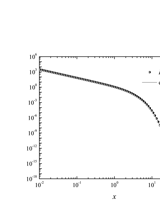
Figure 1: The modified Bessel function, $K_{5/3}(x)$, together with its corresponding fit according to equation (6).

Figure 2: The relative error for the modified Bessel function, $K_{5/3}(x)$, corresponding to the set of coefficients reported by table 1.

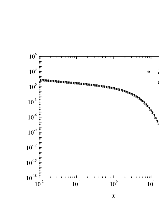
Figure 3: The modified Bessel function, $K_{2/3}(x)$, together with its corresponding fit, according to equation (6).

Figure 4: The relative error for the modified Bessel function, $K_{2/3}(x)$, corresponding to the set of coefficients reported by table 2.

3 Synchrotron Functions

3.1 Definitions

The synchrotron functions, $F(x)$ and $G(x)$, are defined by (Westfold 1959; Jackson 1962; Rybicki & Lightman 1979; Fouka & Ouichaoui 2009):

$$\left\{\begin{array}[]{l}\vspace{0.1cm}\displaystyle{}F(x)=x\int^{\infty}_{x}K_{5/3}(x^{\prime})dx^{\prime}\\ G(x)=xK_{2/3}(x)\end{array}\right..$$ (11)

Function $G(x)$ is called the complementary synchrotron function and is sometimes noted $F_{p}(x)$ (Westfold 1959). The corresponding simplest asymptotic forms of these functions have the following expressions (Westfold 1959; Rybicki & Lightman 1979):

$$F(x)\approx\left\{\begin{array}[]{l}\vspace{0.1cm}\displaystyle{}F_{1}x^{\>1/3}~{}~{}~{}\textnormal{for}~{}~{}~{}x\ll 1\\ \displaystyle{}F_{2}e^{-x}x^{1/2}~{}~{}~{}\textnormal{for}~{}~{}~{}x\gg 1\end{array}\right.$$ (12)

and

$$G(x)\approx\left\{\begin{array}[]{l}\vspace{0.1cm}\displaystyle{}G_{1}x^{\>1/3}~{}~{}~{}\textnormal{for}~{}~{}~{}x\ll 1\\ \displaystyle{}G_{2}e^{-x}x^{1/2}~{}~{}~{}\textnormal{for}~{}~{}~{}x\gg 1\end{array}\right.,$$ (13)

where $F_{1}=\pi 2^{5/3}/\sqrt{3}\Gamma(1/3)$, $F_{2}=\sqrt{\pi/2}$ and $G_{1}=F_{1}/2$ , $G_{2}=F_{2}$.

3.2 Fitting formulae

Function $G(x)$ can be easily derived directly from the fit to function $K_{2/3}(x)$. One has just to multiply the latter by variable $x$. For fitting function $F(x)$ , we proceed in the same way as for the modified Bessel functions, i.e., putting it under the form given by equation (6). We have just to consider the corresponding asymptotic forms given by equation (12). The corresponding fit coefficients are reported in table 4. With these coefficients, the relative error is $<0.26\%$. Function $F(x)$ is plotted in figure 5, together with the corresponding fit while the relative error is reported in figure 6, as a function of variable $x$.

Table 4: Coefficients $a^{(1)}_{k}$ and $a^{(2)}_{k}$ for the synchrotron function $F(x)$.

$k$	$a^{(1)}_{k}$	$a^{(2)}_{k}$
$1$	$-0.97947838884478688$	$-4.69247165562628882\times 10^{-2}$
$2$	$-0.83333239129525072$	$-0.70055018056462881$
$3$	$+0.15541796026816246$	$1.03876297841949544\times 10^{-2}$

0.86 With this set of coefficients, the relative error is $<0.26\%$.

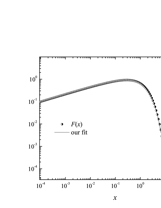
Figure 5: The synchrotron function, $F(x)$, together with its corresponding fit according to equation (6).

Figure 6: The relative error for the synchrotron function, $F(x)$, corresponding to the set of coefficients reported by table 4.

4 Conclusion

We have presented analytical fit formulae with good accuracies for the synchrotron function, $F(x)$, and its complementary function, $G(x)$, based on their known asymptotic forms for low and large $x$-values. We propose these formulae for the aim of directly and simply computing these transcendental functions with avoiding fastidious calculations. The derived general fit formulae can thus be used to evaluate the modified Bessel functions of any order: integer or non integer. Finally, these fit formulae should be of great help for computing quantities of interest to synchrotron radiation such as, e.g., the spectral power and the degree of polarization, both for laboratory and astrophysical applications.