Polarisation control of optically pumped terahertz lasers

Abstract

Optical pumping of excited exciton states in semiconductor quantum wells is a tool for realisation of ultra-compact terahertz (THz) lasers based on stimulated optical transition between excited ($2p$) and ground ($1s$) exciton state. We show that the probability of two-photon absorption by a $2p$-exciton is strongly dependent on the polarisation of both photons. Variation of the threshold power for THz lasing by a factor of 5 is predicted by switching from linear to circular pumping. We calculate the polarisation dependence of the THz emission and identify photon polarisation configurations for achieving maximum THz photon generation quantum efficiency.

Introduction.-Excitons in nanoscale semiconductor materials exhibit low-energy excitations in the range of the exciton binding energy, analogous to inter-level excitations in atoms, yielding infrared and terahertz (THz) transitions. Thus excited exciton ladder states represent a natural system for generating THz radiation and coherence. The demand for development of new compact and efficient coherent terahertz radiation sources is currently rapidly increasing, due to ever growing range of very diverse technological applications in the relatively little-explored THz spectrum of radiation Tonouchi . Towards this goal recently a new scheme of a microcavity based polariton triggered THz laser (THz vertical cavity surface emitting laser (VCSEL)) has been proposed by one of the authors Kavokin , whereby the $2p$ dark quantum well (QW) exciton state is pumped by two-photon absorption using a $cw$ laser beam.

In this Letter we theoretically demonstrate polarisation control of THz emission and of the quantum efficiency for THz photon generation. We consider a THz VCSEL proposed in Ref.( Kavokin ), where the pump beam is split in two. Each of the split beams goes through a polariser, so that the two photons pumping the $2p$ exciton do not necessarily have the same polarisation. We show that by rotating one of the polarisers one can switch on and off the THz laser.

Using crystal symmetry point group theoretical methods Ivchenko we calculate the polarisation dependence of the optical transition matrix element for two-photon excitonic absorption in GaAs/AlGaAs quantum wells, as well as of the intra-excitonic $2p$ to $1s$ THz transition radiative decay rate. This enables us to calculate the polarisation dependence of the quantum efficiency for THz photon generation and thus identify maximum efficiency regimes of operation. The optically pumping scheme to a 2p exciton state by two photons, each of half the energy of the $2p$ exciton state, is shown in Fig. 1.

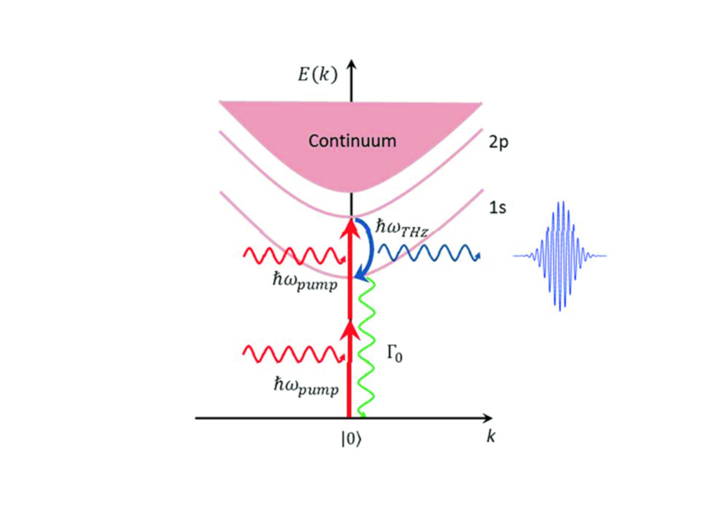
Figure 1: (Color online) Schematic energy-level diagram of two-photon transitions to $2p$ exciton states in a QW. The ground ($1s$) and excited ($2p$ dark) discrete (bound) excitonic states and the exciton (unbound) continuum states are shown. The pumping frequency, $\omega_{pump}$ is half that of the $2p$ exciton state. $\omega_{THz}$ is the center frequency of the emitted THz pulse; $\Gamma_{0}$ - ground ($1s$) state exciton spontaneous emission rate.

Two-photon $p$-exciton absorption.- The quasi-2D (Q2D) exciton wave function at the $\Gamma$ point is given for narrow QWs by Shimizu :

$$\scalebox{0.85}{\mbox{$\displaystyle\Psi_{\lambda}\left({{\bf r}_{e},{\bf r}_{h}}\right)=\frac{{v_{0}}}{{\sqrt{S}}}U_{\lambda}^{\alpha\beta}\left({\bf\rho}\right)\Phi_{c}^{\alpha}\left({z_{e}}\right)\Phi_{v}^{\beta*}\left({z_{h}}\right)u_{c{\bf k}}\left({{\bf r}_{e}}\right)u_{v{\bf k}}^{*}\left({{\bf r}_{h}}\right)e^{i{\bf k}_{||}.{\bf R}_{||}}$}}$$ (1)

where $v_{0}$ is the unit-cell volume, $S$ is the QW area, $\mathbf{R}$ is the centre-of-mass (c.o.m.) co-ordinate, $\mathbf{r}=\mathbf{r}_{e}-\mathbf{r}_{h}$ is the relative motion co-ordinate, $\mathbf{r}({\boldsymbol{\rho}},z)$ and ${\boldsymbol{\rho}}={\boldsymbol{\rho}_{e}}-{\boldsymbol{\rho}_{h}}$ is the in-plane relative motion co-ordinate, the $z$ axis is taken normal to the QW layers. $\alpha,\beta$ are subband indices and $\Phi_{c(v)}^{\alpha}$ is the $\alpha$-subband envelope function of the conduction (valence) band; $U_{\lambda}^{\alpha\beta}\left({\mathbf{r}_{e}-\mathbf{r}_{h}}\right)$ is the envelope function of the 2D exciton associated with subbands $\alpha$ of the electron and $\beta$ of the hole; $\lambda=\left({n,m}\right)$ is the 2D exciton quantum number, labelling the discrete excitonic states ($n=1,2,...,$ $\left|m\right|<n$); $u_{c\mathbf{k}},u_{v\mathbf{k}}$ are the periodic parts of the Bloch wave function for conduction and valence bands, correspondingly; the exciton c.o.m. wave vector, $\mathbf{k}_{||}\approx 0$, is on the order of the photon wave vector. Consider the case of allowed conduction-to-valence band dipole optical transition at the $\Gamma$ point. In cubic crystals the conservation of parity upon absorption of two photons requires the final excitonic state to have the same parity as the valence band, therefore the final exciton is in a $p$-state. The TPA probability is given by:

$$W_{TPA}=\frac{{2\pi}}{\hbar}\sum\limits_{if}{\left|{V_{if}}\right|}^{2}S_{f}\left(E\right)$$ (2)

where $S_{f}$ is the final density of states and the momentum, p, matrix element, $V_{if}$, between the initial and final states is given by Mahan :

reflecting the order of absorption of the first photon with polarisation vector ${\boldsymbol{\varepsilon}}_{1}$, energy $\hbar\omega_{1}$ and vector potential $A_{1}$ and the second - with polarisation vector ${\boldsymbol{\varepsilon}}_{2}$, energy $\hbar\omega_{2}$ and vector potential $A_{2}$. Since the TPA is a two-step process, one should sum over all intermediate states $\left|l\right\rangle$ with energy $E_{l}$. The first matrix element has been calculated by Elliott Elliott in the 3D case and for the quasi-2D case here considered reads:

$$\left\langle l\right|\hat{\varepsilon}_{\alpha}.\mathbf{p}\left|i\right\rangle=\sqrt{S}\Psi_{\lambda}^{*}\left(0\right)\left\langle c\right|\hat{\varepsilon}_{\alpha}.\mathbf{p}\left|v\right\rangle$$ (4)

$$=v_{0}U_{\lambda}^{\alpha\beta}\left(0\right)\Phi_{c}^{\alpha}\left({z_{e}}\right)\Phi_{v}^{\beta*}\left({z_{h}}\right)\left\langle c\right|\mathbf{p}\left|v\right\rangle$$

where $\mathbf{\hat{\varepsilon}}_{\alpha}$, $\alpha=1,2$ is the photon polarisation vector, $\Psi_{\lambda}(0)$ is the relative motion exciton wave function, given by Eq.(1), evaluated at $\mathbf{r=0}$, and the interband matrix element $\left\langle c\right|\hat{\varepsilon}_{\alpha}.\mathbf{p}\left|v\right\rangle$ is given by:

$$\left\langle c\right|\mathbf{p}\left|v\right\rangle=\frac{1}{{v_{0}}}\int\limits_{cell}{d^{3}ru_{c}^{*}\left(\mathbf{r}\right)}\frac{\hbar}{i}\nabla u_{v\mathbf{\hat{z}}}\left(\mathbf{r}\right)$$ (5)

The second matrix element entering Eq.(3) is between hydrogenic-type exciton states and can be written as:

$$\scalebox{0.85}{\mbox{$\displaystyle\frac{1}{m}\left\langle f\right|\hat{\varepsilon}_{\beta}.{\bf p}\left|l\right\rangle=\frac{1}{{\bar{\mu}_{\xi}}}\int{d^{3}r\,}\Psi_{\delta}^{\alpha\beta*}\left({\bf r}\right)\left({{\bf\hat{\varepsilon}}_{\beta}.{\bf p}}\right)\Psi_{\lambda}^{\alpha\beta}\left({\bf r}\right)$}}$$ (6)

$$\scalebox{0.85}{\mbox{$\displaystyle=\frac{1}{{\bar{\mu}_{\xi}}}\int{d^{3}r\,}U_{\delta}^{\alpha\beta*}\left({\bf\rho}\right)\Phi_{c}^{\alpha*}\left({z_{e}}\right)\Phi_{v}^{\beta}\left({z_{h}}\right)\left({{\bf\hat{\varepsilon}}_{\beta}.{\bf p}}\right)U_{\lambda}^{\alpha\beta}\left({\bf\rho}\right)\Phi_{c}^{\alpha}\left({z_{e}}\right)\Phi_{v}^{\beta*}\left({z_{h}}\right)$}}$$

where $m$ is the free electron mass and ${\bar{\mu}_{\xi}}$ is the reduced exciton mass along $\xi$-direction in the QW plane. Introducing a special notation for the matrix element, summed over the intermediate states, according to:

$$\scalebox{0.85}{\mbox{$\displaystyle I_{\delta}\left({\alpha,\beta}\right)=\int{d^{3}r\,}U_{\delta}^{\alpha\beta*}\left({\bf\rho}\right)\Phi_{c}^{\alpha*}\left({z_{e}}\right)\Phi_{v}^{\beta}\left({z_{h}}\right)\left({{\bf\hat{\varepsilon}}_{\beta}.{\bf p}}\right)$}}$$ (7)

$$\scalebox{0.85}{\mbox{$\displaystyle\times\sum\limits_{\lambda}{\frac{{U_{\lambda}^{\alpha\beta}\left({\bf\rho}\right)U_{\lambda}^{\alpha\beta*}\left(0\right)}}{{E_{\lambda}+E_{G}-\hbar\omega_{\alpha}}}}\Phi_{c}^{\alpha*}\left({z_{e}}\right)\Phi_{v}^{\beta}\left({z_{h}}\right)\Phi_{c}^{\alpha}\left({z_{e}}\right)\Phi_{v}^{\beta*}\left({z_{h}}\right)$}}$$

where $E_{G}$ is the direct interband energy gap, the total matrix element can be written as:

Let us define a 2D reduced Coulomb Green’s function:

$$G\left({\boldsymbol{\rho},\boldsymbol{\rho^{\prime}}}\right)=\sum\limits_{\lambda}{\frac{{U_{\lambda}^{\alpha\beta}\left(\boldsymbol{\rho}\right)U_{\lambda}^{\alpha\beta\ast}\left({\boldsymbol{\rho}^{\prime}}\right)}}{{E_{\lambda}-\Omega}}}$$ (9)

where $E_{\lambda}$ is the exciton hydrogenic energy as measured from the conduction-band edge and $\Omega=-E_{G}+\hbar\omega_{\alpha}<0$. A closed form of the reduced Green’s function for an unscreened exciton in 3D (N-D) has been derived in Hostler (Blinder ) and in the 2D limit of interest is given in Zimmermann :

where ${a_{B}^{\ast}}$ is the 3D exciton Bohr radius, $\gamma$ is the Euler’s constant and $\kappa_{\alpha}^{2}=\frac{{E_{B}}}{{E_{G}-\hbar\omega_{\alpha}}}$ with $E_{B}\equiv Ry^{\ast}$ – the exciton binding energy.  Introducing cylindrical co-ordinates and the overlap integral of the subband envelope wave functions:

$$I_{\alpha\beta}=\left\langle{\Phi_{c}^{\alpha}\left(z\right)}\right|\left.{\Phi_{v}^{\beta}\left(z\right)}\right\rangle=\int{dz}\,\Phi_{c}^{\alpha\ast}\left(z\right)\Phi_{v}^{\beta}\left(z\right)$$ (11)

and momentum matrix element along $z$-direction:

$$P_{\alpha\beta}=\left\langle{\Phi_{c}^{\alpha}\left(z\right)}\right|p_{z}\left|{\Phi_{v}^{\beta}\left(z\right)}\right\rangle=\int{dz}\,\Phi_{c}^{\alpha\ast}\left(z\right)\frac{\hbar}{i}\frac{\partial}{{\partial z}}\Phi_{v}^{\beta}\left(z\right)$$ (12)

the general expression for the sum over intermediate states can be recast as:

$$\begin{array}[]{l}I_{\delta}\left({\alpha,\beta}\right)=-i\hbar\frac{{v_{0}^{2}}}{S}\left[{I_{\alpha\beta}\int{d^{2}\rho U_{\delta}^{\alpha\beta\ast}\left(\rho\right)\left({\mathbf{\hat{\varepsilon}}_{\beta}.\mathbf{\hat{\boldsymbol{\rho}}}}\right)\frac{{\partial G\left({\rho,0}\right)}}{{\partial\rho}}}}\right.\\ \left.{+P_{\alpha\beta}\int{d^{2}\rho U_{\delta}^{\alpha\beta\ast}\left(\rho\right)\left({\mathbf{\hat{\varepsilon}}_{\beta}.\mathbf{\hat{z}}}\right)G\left({\rho,0}\right)}}\right]\\ \end{array}$$ (13)

where $\boldsymbol{\hat{\rho}}=\frac{{\boldsymbol{\rho}}}{{\left|{\boldsymbol{\rho}}\right|}}$ and ${\mathbf{\hat{z}}}$ are unit vectors.

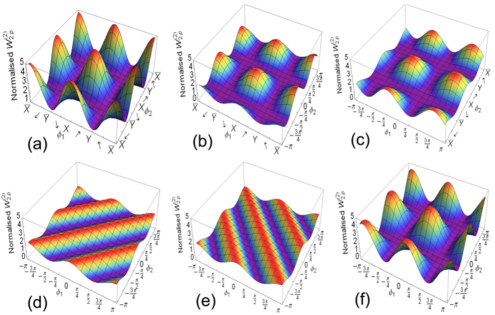
Figure 2: (Color online) 3D surface plots of the normalised excitonic TPA against polar angles of ${\bf\hat{\varepsilon}}_{1}$ and ${\bf\hat{\varepsilon}}_{2}$ in the QW plane at specific phase shifts $\delta_{1},\delta_{2}$. (a) co-linearly polarised photons $\delta_{\mathrm{1}}=0,\pm\pi$;  $\delta_{2}=0,\pm\pi$; (b) $1^{st}$ linear – $2^{nd}$ $\sigma^{+}$ circularly polarised photon $\delta_{\mathrm{1}}=0;\,\delta_{2}=\frac{\pi}{2}$; (c) $1^{st}$ $\sigma^{+}$ circularly polarised photon – $2^{nd}$ linearly polarised photon $\delta_{\mathrm{1}}=\frac{\pi}{2};\,\delta_{2}=0$; (d) $\sigma^{+}$– $\sigma^{+}$ or $\sigma^{-}$– $\sigma^{-}$ co-circularly polarised photons $\delta_{\mathrm{1}}=\pm\frac{\pi}{2};\,\delta_{2}=\pm\frac{\pi}{2}$; (e) $\sigma^{+}$– $\sigma^{-}$ or $\sigma^{-}$– $\sigma^{+}$ counter-circularly polarised photons $\delta_{\mathrm{1}}=\pm\frac{\pi}{2};\,\delta_{2}=\mp\frac{\pi}{2}$; (f) co-left-elliptically polarised photons $\delta_{\mathrm{1}}=-\frac{\pi}{6};\,\delta_{2}=-\frac{\pi}{8}$.

For VCSEL configuration and normal incidence geometry we choose $\mathbf{\hat{\varepsilon}}_{\beta}\bot z$ and therefore the second term in Eq. (13) vanishes. The derivative of the Green’s function can be easily carried out using Eq.(10). We take for the exciton relative motion wave function the 2D hydrogen atom wave function for bound exciton states Shinada&Sugano , Koch&Haug :

$$\scalebox{0.85}{\mbox{$\displaystyle U_{nm}^{\alpha\beta}\left({\boldsymbol{\rho}}\right)=N_{nm}$}}\left({\frac{{2\rho}}{{a_{B}^{*}\left({n-\frac{1}{2}}\right)}}}\right)^{\left|m\right|}e^{-\frac{\rho}{{a_{B}^{*}\left({n-\frac{1}{2}}\right)}}}$$ (14)

$$\scalebox{0.85}{\mbox{$\displaystyle\times L_{n+\left|m\right|-1}^{2\left|m\right|}\left({\frac{{2\rho}}{{a_{B}^{*}\left({n-\frac{1}{2}}\right)}}}\right)e^{im\phi}$}},\,\,\,\,\,\,\,\,n=1,2,3,...,\left|m\right|<n$$

where $N_{nm}=\left[{\frac{{\left({n-1-\left|m\right|}\right)}}{{\pi a_{B}^{*2}\left({n-\frac{1}{2}}\right)^{3}\left[{\left({n-1+\left|m\right|}\right)!}\right]^{3}}}}\right]^{1/2}$ and $L_{n}^{\alpha}\left(x\right)$ – associated Laguerre polynomials Abramowitz&Stegun .

Introducing polar co-ordinates $\left({\rho,\varphi}\right)$ we obtain for TPA to $2p$-exciton states with $n=1,m=\pm 1$:

$$I_{2,1}\left({\alpha,\beta}\right)=\frac{{4\hbar I_{\alpha\beta}}}{{3\pi i\sqrt{3\pi}\kappa_{\alpha}a_{B}^{*3}E_{B}}}J_{p,2}\left({\kappa_{\alpha}}\right)$$ (15)

where $E_{B}=\frac{{\hbar^{2}}}{{2\bar{\mu}_{\xi}a_{B}^{*2}}}$ is the exciton binding energy and the integral, $J_{p,2}\left({k_{\alpha}}\right)=-\frac{{9\left({143+36\ln\left({\frac{2}{3}}\right)}\right)}}{{2048}}a_{B}^{*3}\kappa_{\alpha}^{3}$.

Substituting in Eq. (8) the excitonic two-photon absorption matrix element is obtained:

$$V_{fi}=\frac{{v_{0}^{2}}}{\sqrt{S}}\frac{{e^{2}}}{{mc^{2}}}A_{1}A_{2}\frac{{4\hbar I_{\alpha\beta}}}{{3\pi i\sqrt{3\pi}}}\frac{1}{{E_{B}a_{B}^{*2}}}J_{eff,2}\left\langle c\right|\mathbf{p}\left|v\right\rangle$$ (16)

where we have defined effective matrix element for cubic crystals, using the invariance of the interband matrix element $M=\left\langle c\right|\mathbf{p}\left|v\right\rangle$ under crystal point symmetry group transformations Inoue&Toyozawa , Mahan , Ivchenko , Heine :

$$\scalebox{0.85}{\mbox{$\displaystyle J_{eff,2}^{2}=\frac{1}{2}\left({{\bf\hat{\varepsilon}}_{1}\times{\bf\hat{\varepsilon}}_{2}}\right)^{2}\left|{J_{p,2}\left({k_{1}}\right)-J_{p,2}\left({k_{2}}\right)}\right|^{2}$}}$$ (17)

$$\scalebox{0.85}{\mbox{$\displaystyle+\frac{1}{2}\left[{1+\left({{\bf\hat{\varepsilon}}_{1}.{\bf\hat{\varepsilon}}_{2}}\right)^{2}}\right]\left|{J_{p,2}\left({k_{1}}\right)+J_{p,2}\left({k_{2}}\right)}\right|^{2}$}}$$

$$\scalebox{0.85}{\mbox{$\displaystyle=\frac{{C_{1}^{2}}}{2}\left\{{\left({{\bf\hat{\varepsilon}}_{1}\times{\bf\hat{\varepsilon}}_{2}}\right)^{2}\left|{k_{1}^{2}-k_{2}^{2}}\right|^{2}+\left[{1+\left({{\bf\hat{\varepsilon}}_{1}.\,{\bf\hat{\varepsilon}}_{2}}\right)^{2}}\right]\left|{k_{1}^{2}+k_{2}^{2}}\right|^{2}}\right\}$}}$$

where $C_{1}=-\frac{{9\left({143+36\ln\left({\frac{2}{3}}\right)}\right)}}{{2048}}$.

Our pumping scheme envisages two photons each with half the energy of the $2p$-exciton state: $\hbar\omega_{1}=\hbar\omega_{2}=\hbar\omega=\frac{{E_{2p}}}{2}$ and $k_{1}^{2}=k_{2}^{2}=k^{2}=\frac{{2E_{B}}}{{2E_{G}-E_{2p}}}$, therefore the first term in Eq. (17) vanishes and from Eq. (2) we get for the TPA probability to $2p$-exciton states in [$\mathrm{s^{-1}m^{-2}}$]:

where $S_{2p}^{c1,hh1}$ is the final $2p$-exciton density of states per unit area for a heavy-hole exciton (c1-hh1) and the coefficient $K_{TPA}$ for an infinite quantum well, is given by:

$$K_{TPA}=\frac{{128\pi e^{4}A_{1}^{2}A_{2}^{2}v_{0}^{2}}}{{\hbar\bar{\mu}_{\xi}^{2}m^{2}c^{4}SL_{z}^{2}E_{B}^{2}}}$$ (19)

The photon polarisation vectors ${\mathbf{\hat{\varepsilon}}_{1},\mathbf{\hat{\varepsilon}}_{2}}$ with polar angles $\varphi_{1},\varphi_{2}$ and phase shifts $\delta_{1},\delta_{2}$ correspondingly, lie in the QW plane. 3D plots of the exciton TPA probability are shown in Fig. 2 for different polarisations of the two pumping photons.

We suggest adding an external THz cavity at the VCSEL output that will filter out the linear polarisation of the emitted THz radiation, and will thus constitute our reference frame, fixing the direction of our co-ordinate system x-axis. We shall assume that the generated THz mode is X-polarised. By inspection of Fig. 2 one can see that maximum ($5$-fold) increase of the two-photon absorption rate with respect to $YY$ polarisation is achieved for linearly $XX,X\bar{X},\bar{X}X,\bar{X}\bar{X}$ polarised photons (Fig. 2(a)). The two-photon absorption rate can increase by a factor of $3$ for linearly-circularly or circularly-linearly polarised photons (Fig 2(b,c)); by a factor of $2$ for both circularly polarised (Fig. 2 (d,e)), by a factor close to $5$ (but always less than the one for linear polarisation) for elliptically polarised photons (Fig. 2 (f)). Our results show that changing polarisation from $YY$ to $XX$, passing through circularly and elliptically polarised pumping, one can vary the lasing threshold by a factor of 5.

Intra-excitonic $2p\rightarrow 1s$ transition probability.- We calculate next the polarisation dependence of the $2p\rightarrow 1s$ photon intra-excitonic transition rate, generating THz emission (Fig. 1). We are interested in the optical transition matrix element between initial two-fold degenerate state $\Psi_{\delta}$ with $\delta=(n=2,m=\pm 1)=(2,p)$ and final state $\Psi_{\lambda}$ with $\lambda=(n=1,m=0)=(1,s)$. The matrix element is of the second type Eq.(6) and for normal incidence geometry $(\boldsymbol{\hat{\varepsilon}}\bot\boldsymbol{\hat{z}})$ and exciton wave functions, given by Eqs. (1),(14), we obtain:

$$\scalebox{0.75}{\mbox{$\displaystyle M_{lf}=\frac{{v_{0}^{2}}}{S}\left({\frac{{\ -8\,\hbar}}{i}}\right)\left({\frac{m}{{\bar{\mu}_{\xi}}}}\right)I_{\alpha\beta}^{2}\left({\frac{1}{{3\sqrt{3}}}}\right)\frac{{2\sqrt{2}}}{{3\pi a_{B}^{*4}}}\Phi\left(\varphi\right)\int{d\rho\,\rho^{2}}e^{-\frac{{8\rho}}{{3a_{B}^{*}}}}L_{2}^{2}\left({\frac{{4\rho}}{{3a_{B}^{*}}}}\right)$}}$$ (20)

where we have introduced polar co-ordinates and the angular dependence is given by: $\Phi\left(\varphi\right)=\cos\varphi\,e^{\mp i\varphi}$. The integration over $\rho$ is easily performed, giving: $\frac{{81}}{{512}}a_{B}^{*3}$. Finally, the $2p\rightarrow 1s$ intra-excitonic optical transition rate for an infinite QW is given by:

$$W_{2p\to 1s}^{(2)}=\frac{{27}}{{512}}K_{OPA}^{THz}\frac{{\hbar^{2}}}{{\pi^{2}a_{B}^{*2}}}I_{\alpha\beta}^{4}S_{1s}\left(E\right)\Phi^{2}\left(\varphi\right)$$ (21)

where $S_{1s}(E)$ is the final ($1s$) state density of states and the one-photon THz emission coefficient is given by:

$$K_{OPA}^{THz}=\frac{{16\pi}}{\hbar}\left({\frac{e}{{\bar{\mu}_{\xi}c}}}\right)^{2}\frac{{v_{0}^{2}A_{THz}^{2}}}{{L_{z}^{4}S}}$$ (22)

where $A_{THz}$ is the THz photon vector potential, expressed in terms of the THz emission intensity, $I_{THz}$ as: $A_{THz}=\left({\frac{{2\pi cI_{THz}}}{{n\omega_{THz}^{2}}}}\right)^{1/2}$, where $n$ is the refractive index and $\omega_{THz}=\frac{{E_{2p}-E_{1s}}}{\hbar}$.

The polarisation dependence of the THz emission rate can be inferred from the angular dependence: for linear (e.g. along x-axis) polarisation of the emitted THz photon ($\mathbf{\hat{\varepsilon}}||\,\mathbf{\hat{x}}$), $\Phi^{2}\left(\varphi\right)=1$, for y-linear $\mathbf{\hat{\varepsilon}}||\,\mathbf{\hat{y}}$, $\Phi^{2}\left(\varphi\right)=0$ and therefore there is no THz emission, and for circularly polarised THz photon, $\Phi^{2}\left(\varphi\right)=\frac{1}{2}$, the corresponding THz emission rate is half of the one for x-linear polarisation.

Quantum efficiency.- The quantum efficiency of THz radiation generation can be defined as the ratio of the THz photon generation rate and the two-photon absorption rate by a $2p$-exciton and is proportional to the ratio of the squares of the oscillator strengths, $G$ and $g$, of the $2p\rightarrow 1s$ and $|0\rangle\rightarrow|2p\rangle$ transitions Kavokin , which can be expressed in terms of the transition probability Yariv :

$$\scalebox{0.8}{\mbox{$\displaystyle G^{2}\equiv f_{2p\to 1s}=\frac{{6\pi c^{3}\varepsilon\bar{\mu}_{\xi}S}}{{\omega_{THz}^{2}n^{3}e^{2}}}W_{2p\to 1s}^{\left(2\right)}$}}$$ (23)

$$\scalebox{0.8}{\mbox{$\displaystyle g^{2}\equiv f_{2p}=\frac{{6\pi c^{3}\varepsilon\bar{\mu}_{\xi}S}}{{\omega_{2p}^{2}n^{3}e^{2}}}W_{2p}^{\left(2\right)}$}}$$

where $\omega_{2p}=\frac{{E_{2p}}}{\hbar}$.

Using Eq.(18) and Eq.(21), after some algebra one can obtain for the normalised quantum efficiency:

where the polarisation dependence is given by:

$$\scalebox{0.85}{\mbox{$\displaystyle P\left({{\bf\hat{\varepsilon}}_{1},{\bf\hat{\varepsilon}}_{2},{\bf\hat{\varepsilon}}}\right)=\frac{{\cos^{2}\left(\varphi\right)}}{{1+\left({\cos\varphi_{1}\cos\varphi_{2}+\cos\left({\varphi_{1}+\delta_{1}}\right)\cos\left({\varphi_{2}+\delta_{2}}\right)}\right)^{2}}}$}}$$ (25)

and $\varphi$ is the polar angle of the THz photon polarisation vector.

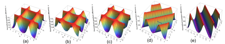
Figure 3: (Color online) 3D surface plots of the normalised quantum efficiency of THz photon generation against polar angles of the pumping photons polarisation vectors in the QW plane at different phase shifts $\delta_{1},\delta_{2}$ at linear, $\phi=0,\pm\pi$ polarisation of the emitted THz radiation (a) co-linearly polarised photons;(b) $1^{st}$ linear-$2^{nd}$ circularly polarised photon; (c) $1^{st}$ circular –$2^{nd}$ linearly polarised; (d) $\sigma^{+}$–$\sigma^{+}$ or $\sigma^{-}$–$\sigma^{-}$ co-circularly polarised photons; (e) $\sigma^{+}$–$\sigma^{-}$ or $\sigma^{-}$–$\sigma^{+}$ counter-circularly polarised photons.

We shall assume that the $2p$ exciton excited by two-photon absorption has a lifetime, which is long enough that it loses any memory of the polarisation and phase of the excitation, so that it can emit with any polarisation. We shall consider emission with one particular polarisation (either linear or circular) and all possible choices of polarisation of the two pumping photons.

The quantum efficiency polarisation dependence is shown in Fig. 3 for different polarisation configurations of the two pumping photons at a given (linear) emitted THz photon polarisation. The plots for circular polarisation of the THz radiation look exactly the same but are scaled down by a factor of 2 (not shown), resulting in maximum efficiency $\eta=0.5$. In addition to the results presented in Fig. 3, we should note that for counter-$X\left({\bar{X}}\right)$-linearly polarised pumping photons $\delta_{1}=0\left(\pi\right);\delta_{2}=\pi\left(0\right)$ maximum quantum efficiency $\eta=1$ is achieved for linearly polarised ($\phi=0,\pi$) and $\eta=0.5$ for circularly polarised $(\varphi=\frac{\pi}{4})$ THz emission, unconditionally, for any direction of the linear polarisation of the two pumping photons in the QW plane. Furthermore, if the THz emission is $Y$-linearly polarised, the quantum efficiency $\eta=0$, i.e. no THz radiation should be emitted in this case. Fig. 3 shows that the maximum quantum efficiency $\eta=1$ could be achieved within certain regions in the plane for linearly polarised THz emission for all combinations of linear and circular polarisations of the two pumping photons. Note that in both (circular and linear THz emission polarisation) cases, maximum quantum efficiency is achieved along $YY$ lines for co-linearly polarised photons, for $Y$-polarised first (second) photon in the case of linear-circular (circular-linear) polarisation, or along diagonal lines for co- and counter- circular-circular polarisation of the pumping photons. We emphasise, however, that although maximum quantum efficiency could be achieved both by counter- and co-linearly polarised photons, the quantum efficiency in the former case is constant and does not depend on the direction of the polarisation vectors in the QW plane, while maximum quantum efficiency in the latter case is obtained solely for specific directions of the polarisation vectors in the plane ($YY$).

In order to verify these predictions experimentally, one can envisage pumping of a QW structure with two laser beams having the same frequency (equal to a half of the $2p$-exciton resonance frequency) but different polarisation. These two beams may be generated by the same laser but should propagate through different polarisers before focussing on the sample. In addition we suggest including a delay line between the two parts of the pumping beam, which would provide the phase difference of $\pi$ between them to obtain counter-linearly polarised beams for which unconditional maximum efficiency is predicted. The intensity and polarisation of the THz light emitted by the structure could be measured as a function of intensities and polarisations of the two pumping beams. As reference experiments one can measure the intensity of THz emission with one of the pump beams switched off. Analysing the results of such experiments one should bear in mind that the two photons used to generate a $2p$-exciton may originate from the same beam as well as from different beams. Comparing the spectra obtained with both beams switched on with those obtained with only the first or only the second beam switched on, one can extract the signal generated by absorption of the two photons coming from different beams and thus having different polarisations.

Conclusions.- We have developed a theory of the two-photon absorption to $p$-exciton states in QWs and calculated the polarisation dependence of two-photon transition probability, using crystal symmetry point group methods. We show that the two-photon transition rate is strongly dependent on the polarisation of both photons and our model predicts variation of the lasing threshold by a factor of $5$ by switching from $YY$ to co-linearly $XX$-polarised pumping. We calculated the polarisation dependence of the intra-excitonic THz emission and the quantum efficiency for THz photon generation. Maximum quantum efficiency is predicted for counter-linearly polarised pumping photons and linearly polarised THz emission. Conditions for achieving maximum quantum efficiency for different polarisations of the pumping photons are identified, thereby opening routes for polarisation control of the THz VCSEL and a range of new applications entailed from it.

We thank Prof. E. L. Ivchenko for valuable discussions. AK acknowledges financial support from the EPSRC Established Career Fellowship grant.

References

• (1) M. Tonouchi, Nature Photonics, 1, 97 (2007)
• (2) A. V. Kavokin, I. A. Shelykh, T. Taylor, and M. M. Glazov, Phys. Rev. Lett. 108, 197401 (2012)
• (3) E. L. Ivchenko and G. E. Pikus, Superlattices and Other Heterostructures (Springer-Verlag, Berlin, 1997).
• (4) A. Shimizu, Phys. Rev. B 40, 1403 (1989)
• (5) G. D. Mahan, Phys. Rev. 170, 825 (1968)
• (6) R. J. Elliott, Phys. Rev. 108, 1384 (1957)
• (7) L. C. Hostler, Journal of Math. Phys., 5, 591 (1964); L. C. Hostler, Phys. Rev. 178, 178 (1969)
• (8) S. M. Blinder, J. Math. Phys. 25, 905 (1984)
• (9) R. Zimmermann, Phys. Stat. Sol. (b), 146, 371 (1988)
• (10) M. Shinada and S. Sugano, J. of the Phys. Soc. of Japan, 21,1936 (1966)
• (11) H. Haug and S. W. Koch, Quantum theory of the optical and electronic properties of semiconductors (World Scientific, 1994)
• (12) Handbook of Mathematical Functions, Ed. M Abramowitz and I. A. Stegun (US Department of Commerce, National Bureau of Standards, Washington, D.C., 1964), Appl. Math. Ser. 55
• (13) Quantum Electronics 3rd edition, A. Yariv (John Wiley), 1988
• (14) M. Inoue and Y. Toyozawa, J. of the Phys. Soc. of Japan, 20, 363 (1965)
• (15) V. Heine, Group theory in quantum mechanics, (Dover Publications, 1993)