Chaotic dynamics of the Bianchi IX universe in Gauss-Bonnet gravity

Abstract

We investigate the dynamics of closed FRW universe and anisotropic Bianchi type-IX universe characterized by two scale factors in a gravity theory including a higher curvature (Gauss-Bonnet) term. The presence of the cosmological constant creates a critical point of saddle type in the phase space of the system. An orbit starting from a neighborhood of the separatrix will evolve toward the critical point, and it eventually either expands to the de Sitter space or collapses to the big crunch. In the closed FRW model, the dynamics is reduced to hyperbolic motions in the two-dimensional center manifold, and the system is not chaotic. In the anisotropic model, anisotropy introduces the rotational mode, which interacts with the hyperbolic mode to present a cylindrical structure of unstable periodic orbits in the neighborhood of the critical point. Due to the non-integrability of the system, the interaction of rotational and hyperbolic modes makes the system chaotic, making it impossible for us to predict the final fate of the universe. We find that the chaotic dynamics arises from the fact that orbits with even small perturbations around the separatrix oscillate in the neighborhood of the critical point before finally expanding or collapsing. The chaotic character is also evidenced by the fractal structures in the basins of attraction.

I Introduction

The pioneering work of Belinskii, Khalatnikov, and Lifshitz Belinskii et al. (1969) has shown that anisotropic Bianchi type-IX universes could exhibit chaotic dynamics as it approaches the cosmological singularity $\left(t\rightarrow 0\right)$. The anisotropic Bianchi IX universe, as it approaches the singularity, exhibits an oscillatory mode consisting of an infinite sequence of Kasner eras, during which two scale factors oscillate and the remaining scale factor decreases monotonically. Independently, Misner Misner (1969) also suggested a chaotic approach to initial singularity in his Mixmaster universe (vacuum Bianchi IX universe characterized by three scale factors).

While the aspect of chaotic dynamics helped deepen our understanding of singularities in general relativity, there have been significant challenges in finding an invariant measure of chaos. A standard measure of chaos is the Lyapunov exponent, and a debate started on whether or not the Mixmaster universe is chaotic, when some studies found zero Lyapunov exponent for the Mixmaster universe, while others found a positive Lyapunov exponent Francisco and Matsas (1988); Burd et al. (1991); Berger (1991). The conflict was resolved when it was realized Rugh (1990) that Lyapunov exponent is coordinate dependent and therefore is not a reliable measure of chaos in general relativity.

Cornish and Levin Cornish and Levin (1996) demonstrated the appearance of chaos in the dynamics of the Friedmann-Robertson-Walker (FRW) models with a cosmological constant and scalar fields conformally coupled to the geometry. The presence of the cosmological constant creates a saddle point in the phase space, and the separatrix connects this saddle point to other critical points. When there are interactions between the geometry with the scalar fields, the separatrix breaks up and becomes fractal. The work by de Oliveira, Soares, and Stuchi De Oliveira et al. (1997) emphasized that even small perturbations induces the breaking of highly unstable separatrix. The presence of a positive cosmological constant and a perfect fluid creates a saddle-center in the phase space, and non-integrability of the system induces distortion and twisting of the topology of homoclinic cylinders in the neighborhood of the critical point. The fractal and topological structures are coordinate-independent and thus provide invariant characterization of chaos in relativistic theories.

Regarding such a system as a model of the early universe, a natural question that arises is whether the Einstein gravity is reliable or not. It has been pointed out Brandenberger and Martin (2012) that we might have the trans-Planckian issue; at early stages of inflation, the quantum gravity effects are not necessarily negligible. Previous works on chaotic dynamics in the per-inflationary era focused on Einstein gravity, but as we approach the Planck scale, it is reasonable to expect higher order corrections to the Einstein-Hilbert action. Superstring theory is the leading candidate for a description of physics at such scale. Our goal in this paper is to use an invariant characterization of chaos and investigate the existence of chaotic dynamics in “string-inspired” modified gravity. Our model takes into account the effects of the higher curvature terms that typically arise in the one-loop low-energy effective superstring action. For simplicity we focus on a model in which a scalar field representing the string moduli is non-minimally coupled to the Gauss-Bonnet curvature. For a related work on chaotic dynamics of higher curvature modified gravity, see e.g. Cotsakis et al. (1993).

The Bianchi type-IX models with a scalar field coupled to the Gauss-Bonnet term are studied in somewhat different context of singularity avoidance in Yajima et al. (2000). The new features introduced by our model are a positive cosmological constant and a perfect fluid, which create saddle points in the phase space of the system. Because this method does not work for the case of zero cosmological constant, our work implies that in order for the universe to inflate we need to include a positive cosmological constant in the low-energy effective action. We introduce this modified action in Sec. II. We first consider the closed FRW universe in Sec. III, where the degrees of freedom are the scale factor and a scalar field, and discuss the basic characteristics of the closed FRW model. We introduce anisotropy in the metric in Sec. IV and discuss how anisotropy creates a topological structure of cylinders near the critical point. In Sec. V we present numerical evidence of cylindrical topology, oscillatory behavior around the critical point, and fractal structures in the basins of attraction when small perturbations are introduced in the metric and/or the scalar field. The fractal structures in the basins of attraction, as well as the topology of cylinders, constitute invariant characterization of chaos, and we conclude that chaotic dynamics can arise in our string-inspired model.

II One-loop effective action

We start with the action in the Einstein frame given by Antoniadis et al. (1994); Rizos and Tamvakis (1994); Easther and Maeda (1996); Kawai et al. (1998); Kawai and Soda (1999); Yajima et al. (2000)

$$S=\int\mathrm{d}^{4}x\sqrt{-g}\left[\frac{1}{2}R-\Lambda-\frac{1}{2}\left(\nabla\sigma\right)^{2}-\frac{\lambda}{16}\xi\left(\sigma\right)R_{GB}^{2}\right]\\ +S_{matter}$$ (1)

where $R$ and $\sigma$ are the Ricci scalar curvature and a scalar field, respectively. In our units, the gravitational constant corresponds to $G=1/8\pi$. A positive cosmological constant is necessary for the existence of a saddle point in phase space and the universe to inflate. The Gauss-Bonnet curvature is given by

$$R_{GB}^{2}=R^{2}-4R^{\alpha\beta}R_{\alpha\beta}+R^{\alpha\beta\gamma\delta}R_{\alpha\beta\gamma\delta}$$ (2)

and the function $\xi\left(\sigma\right)$ depends on details of string theory compactified geometry Antoniadis et al. (1992). For example, when $\sigma$ is the dilaton, we have

$$\xi\left(\sigma\right)=e^{\sigma}$$ (3)

In type II superstring, $\sigma$ can be regarded as the modulus of compactified dimensions. The form of $\xi\left(\sigma\right)$ in a particular compactification can be found in Antoniadis et al. (1992, 1994). The function $\xi\left(\sigma\right)$ determines the coupling of $\sigma$ and the geometry, and is expressed with Dedekind $\eta$ function as

$$\xi\left(\sigma\right)=-\ln\left[2e^{\sigma}\eta^{4}\left(ie^{\sigma}\right)\right]$$ (4)

Due to the modular property

$$\eta\left(-\frac{1}{\tau}\right)=\sqrt{-i\tau}\eta\left(\tau\right)$$ (5)

the function $\xi\left(\sigma\right)$ is even in $\sigma$, has a global minimum at $\sigma=0$, and increases exponentially as $\sigma\rightarrow\pm\infty$. We will be interested in the small $\sigma$ behavior in the following sections. We assume for simplicity that $\xi\left(\sigma\right)$ can be approximated as

$$\xi\left(\sigma\right)=\frac{1}{2}\sigma^{2}$$ (6)

III Closed Friedmann-Robertson-Walker universe

We first consider a cosmological model characterized by the scale factor $a\left(t\right)$ with the line element given by

$$\mathrm{d}s^{2}=-\mathrm{d}t^{2}+a^{2}\left(t\right)\left[\left(\omega^{1}\right)^{2}+\left(\omega^{2}\right)^{2}+\left(\omega^{3}\right)^{2}\right]$$ (7)

The Bianchi type-IX invariant one-forms $\omega^{i}$ are given by

$$\omega^{1} =\sin\psi\,\mathrm{d}\theta-\sin\theta\cos\psi\,\mathrm{d}\phi$$

$$\omega^{2} =\cos\psi\,\mathrm{d}\theta+\sin\theta\sin\psi\,\mathrm{d}\phi$$

$$\omega^{3} =\cos\theta\,\mathrm{d}\phi+\mathrm{d}\psi$$ (8)

which are chosen to satisfy $\mathrm{d}\omega^{i}=-\frac{1}{2}{\epsilon^{i}}_{jk}\omega^{j}\wedge\omega^{k}$ and ${\epsilon^{i}}_{jk}$ is the completely antisymmetric tensor $\left({\epsilon^{1}}_{23}=1\right)$. This represents the closed FRW universe with positive curvature $k=+1$. We assume that the matter content is a perfect fluid. The energy-momentum tensor of the perfect fluid can be written in the form

$$T^{\mu\nu}=\left(\rho+p\right)\delta_{0}^{\mu}\delta_{0}^{\nu}+pg^{\mu\nu}$$ (9)

where $\rho$ and $p$ are energy density and pressure, respectively. For simplicity, we assume that the perfect fluid may be represented by “dust,” that is, $\gamma=0$ in the equation of state $p=\gamma\rho$. However, even for general perfect fluids, we can expect similar features Barguine et al. (2001).

For the action (1) the Lagrangian is given by

$$L=\frac{3}{4}a-\Lambda a^{3}-3a\dot{a}^{2}+\frac{1}{2}a^{3}\dot{\sigma}^{2}+\frac{\lambda}{8}\sigma\dot{\sigma}\left(3\dot{a}+4\dot{a}^{3}\right)$$ (10)

where the overdot denotes differentiation with respect to time $t$. The equations of motion are

$$-\frac{1}{4}+\Lambda a^{2}-\dot{a}^{2}-\frac{1}{2}a^{2}\dot{\sigma}^{2}-2a\ddot{a}\\ +\frac{1}{8}\lambda\left(\dot{\sigma}^{2}+4\dot{a}^{2}\dot{\sigma}^{2}+8\sigma\dot{\sigma}\dot{a}\ddot{a}+\sigma\ddot{\sigma}+4\sigma\ddot{\sigma}\dot{a}^{2}\right)=0$$

$$3a^{2}\dot{a}\dot{\sigma}+a^{3}\ddot{\sigma}+\frac{3}{8}\lambda\sigma\ddot{a}\left(1+4\dot{a}^{2}\right)=0$$ (11)

with the Hamiltonian constraint given by

$$H=-3a\dot{a}^{2}-\frac{3}{4}a+a^{3}\Lambda+\frac{3}{8}\lambda\sigma\dot{\sigma}\dot{a}\left(1+4\dot{a}^{2}\right)+\frac{1}{2}a^{3}\dot{\sigma}^{2}+E_{0}=0$$ (12)

where $E_{0}=\rho a^{3}$ corresponds to the total matter content of the model.

We can always decompose a set of second-order differential equations into a set of first-order differential equations by redefining variables. Thus, we get a set of four coupled first-order ordinary differential equations

$$\frac{\mathrm{d}}{\mathrm{d}t}a=\dot{a},\qquad\frac{\mathrm{d}}{\mathrm{d}t}\sigma=\dot{\sigma}$$

$$\frac{\mathrm{d}}{\mathrm{d}t}\dot{a}=8a^{2}\bigg{[}-3\lambda\sigma\dot{\sigma}\dot{a}\left(1+4\dot{a}^{2}\right)\\ +a^{3}\left(8\Lambda-4\dot{\sigma}^{2}\right)+a\left(1+4\dot{a}^{2}\right)\left(-2+\lambda\dot{\sigma}^{2}\right)\bigg{]}\chi$$

$$\frac{\mathrm{d}}{\mathrm{d}t}\dot{\sigma}=\Bigg{\{}-384a^{3}\dot{a}\dot{\sigma}+3\lambda\sigma\bigg{(}-\left(1+4\dot{a}^{2}\right)^{2}\left(-2+\lambda\dot{\sigma}^{2}\right)\\ +4a^{2}\left[-2\Lambda+\dot{\sigma}^{2}+4\dot{a}^{2}\left(-2\Lambda+5\dot{\sigma}^{2}\right)\right]\bigg{)}\Bigg{\}}\chi$$ (13)

where $\chi$ is given by

$$\chi=\frac{1}{64a^{3}\left(2a-\lambda\dot{a}\sigma\dot{\sigma}\right)+3\lambda^{2}\sigma^{2}\left(1+4\dot{a}^{2}\right)^{2}}$$ (14)

The dynamical system (13) admits the static Einstein universe as a solution, which is just the critical point $P$. Its coordinates are given by

$$P:\;a =a_{0}\equiv\frac{1}{2\sqrt{\Lambda}},\;\sigma=\sigma_{0},\;\dot{a}=0,\,\dot{\sigma}=0$$ (15)

where $\sigma_{0}$ is a constant. The critical energy is given by

$$E_{crit}=\frac{1}{4\sqrt{\Lambda}}$$ (16)

When the scalar field is absent and does not interact with the curvature, the equations of motion can be integrated exactly, and the dynamical system admits an invariant manifold $\mathcal{M}$. The invariant manifold $\mathcal{M}$ is defined by

$$\mathcal{M}:\;\sigma=0,\quad\dot{\sigma}=0$$ (17)

and the dynamical system simplifies to an exactly integrable two-dimensional system

$$\frac{\mathrm{d}}{\mathrm{d}t}a=\dot{a}$$

$$\frac{\mathrm{d}}{\mathrm{d}t}\dot{a}=-\frac{1}{8a}-\frac{\dot{a}^{2}}{2a}+\frac{1}{2}\Lambda a$$ (18)

In Fig. 1 we display the phase space portrait of the invariant manifold $\mathcal{M}$ in the $\left(a,\dot{a}\right)$ plane. We introduce the conformal time $\mathrm{d}\eta=\mathrm{d}t/a$ so that the dynamical system (18) becomes regular at $a=0$. The phase space is divided by a separatrix into two types of orbits: those that collapse into the big crunch and those that expand into the de Sitter space. The critical point $P$ intersects the invariant manifold $\mathcal{M}$ at $\sigma_{0}=0$. Furthermore, there are attractors corresponding to stable and unstable de Sitter spaces. When the dynamics is dominated by the cosmological constant $\Lambda$, it can be shown that the scale factor $a\left(t\right)$ expands exponentially and approaches the stable de Sitter attractor as $a\left(t\right)\sim e^{\sqrt{\Lambda/3}t}$.

Figure 1: Phase space portrait of the invariant manifold $\mathcal{M}$ in conformal time $\mathrm{d}\eta=\mathrm{d}t/a$. The orbit $S$ is the separatrix and the point $P$ is the critical point.

Let us now linearize the dynamical equations (13) about the critical point $P$. We move the critical point to the origin by redefining

$$a\rightarrow a+a_{0},\quad \sigma\rightarrow\sigma+0$$

$$\dot{a}\rightarrow\dot{a}+0,\quad \dot{\sigma}\rightarrow\dot{\sigma}+0$$ (19)

then we obtain

$$\frac{\mathrm{d}}{\mathrm{d}t}\begin{pmatrix}a\\ \sigma\\ \dot{a}\\ \dot{\sigma}\end{pmatrix}=A_{0}\begin{pmatrix}a\\ \sigma\\ \dot{a}\\ \dot{\sigma}\end{pmatrix}+\begin{pmatrix}\text{higher}\\ \text{order}\\ \text{terms}\end{pmatrix}$$ (20)

where the constant matrix associated with linearizing the system (13) about the critical point $P$ is given by

$$A_{0}=\begin{pmatrix}0&0&1&0\\ 0&0&0&1\\ \Lambda&0&0&0\\ 0&0&0&0\end{pmatrix}$$ (21)

The matrix (21) has four eigenvalues

$$\lambda_{1,2}=\pm\sqrt{\Lambda},\quad\lambda_{3,4}=0^{2}$$ (22)

According to the center manifold theorem Wiggins (2003), the study of the dynamics near the critical point can be reduced to the study of the dynamics restricted to the associated two-dimensional invariant manifolds $W^{c}\left(0\right)$ near the critical point. Without actually calculating the center manifold, we argue as follows. Under the coordinate transformation

$$\begin{pmatrix}a\\ \sigma\\ \dot{a}\\ \dot{\sigma}\end{pmatrix}=\begin{pmatrix}0&0&-\frac{1}{\sqrt{\Lambda}}&\frac{1}{\sqrt{\Lambda}}\\ 1&0&0&0\\ 0&0&1&1\\ 0&1&0&0\end{pmatrix}\begin{pmatrix}u_{1}\\ u_{2}\\ u_{3}\\ u_{4}\end{pmatrix}$$ (23)

the matrix (21) assumes the Jordan canonical form

$$J=\begin{pmatrix}0&1&0&0\\ 0&0&0&0\\ 0&0&-\sqrt{\Lambda}&0\\ 0&0&0&\sqrt{\Lambda}\end{pmatrix}$$ (24)

Thus the four-dimensional system (13) restricted on the center manifold $W^{c}\left(0\right)$ is a two-dimensional vector field whose linear part is given by

$$\begin{pmatrix}0&1\\ 0&0\end{pmatrix}$$ (25)

Bogdanov Bogdanov (1975) has shown that the system which has a linear part (25) is locally topologically equivalent near the critical point to the normal form

$$\dot{v}_{1}=v_{2}$$

$$\dot{v}_{2} = \beta_{1}+\beta_{2}v_{2}+v_{1}^{2}+\gamma v_{1}v_{2}$$ (26)

where $\gamma=\pm 1$. The dynamics of (26) is not qualitatively changed by the higher order terms in the normal form. The normal form (26) has no homoclinic or periodic solutions for $\beta_{1}>0$. If we rescale the variables and parameters as

$$v_{1}=\epsilon^{2}q_{1},\quad v_{2}=\epsilon^{3}p_{1},\quad\beta_{1}=\epsilon^{4}\mu,\quad\beta_{2}=\epsilon^{2}$$ (27)

where $\epsilon>0$ and rescale the time as

$$t\rightarrow\frac{t}{\epsilon}$$ (28)

then the system becomes

$$\dot{q}_{1}=p_{1}$$

$$\dot{p}_{1}=\mu+q_{1}^{2}+\epsilon\left(p_{1}+\gamma q_{1}p_{1}\right)$$ (29)

For $\epsilon=0$, the rescaled equations become exactly integrable Hamiltonian system with the Hamiltonian given by

$$H\left(q_{1},p_{1}\right)=\frac{p_{1}^{2}}{2}+\frac{q_{1}^{3}}{3}+\mu q_{1}$$ (30)

where $\mu$ is a parameter with $\mu>0$ corresponding to the near-zero eigenvalues being real. For $\mu<0$ there exist homoclinic solutions. However, we restrict our attention to only the hyperbolic motions and do not consider the homoclinic orbits, because homoclinic orbits extend to $a<0$ region of the phase space, which does not have a physical meaning.

In the parlance of nonlinear dynamical systems theory, this is the Bogdanov-Takens bifurcation. To perform a global analysis that includes the effect of the $\mathcal{O}\left(\epsilon\right)$ part of (29) on this integrable structure, Melinkov’s method Wiggins (2003) can be used. A detailed description of bifurcation diagrams and phase portraits of the Bogdanov-Takens bifurcation can be found elsewhere (cf. Arnold and Levi (1988)) and need not be repeated here.

What the above linear analysis shows is that although we could expect simple hyperbolic motion of the planar Bogdanov-Takens bifurcation, we do not expect chaotic dynamics in our closed FRW model. As we will see in Sec. IV, the chaotic dynamics, especially the rotational mode of the oscillatory Mixmaster dynamics, arises from the presence of imaginary eigenvalues of the linearized matrix.

IV Axisymmetric Bianchi IX Universe

Chaos is expected to come from the anisotropy of the universe. For simplicity, we restrict our attention to two distinct scale factors $a\left(t\right)$ and $b\left(t\right)$ and consider an axisymmetric Bianchi IX cosmological model with the line element

$$ds^{2}=-dt^{2}+a^{2}\left(t\right)\left[\left(\omega^{1}\right)^{2}+\left(\omega^{2}\right)^{2}\right]+b^{2}\left(t\right)\left(\omega^{3}\right)^{2}$$ (31)

For the action (1) the Lagrangian is given by

$$L=b-\Lambda a^{2}b-\frac{b^{3}}{4a^{2}}-b\dot{a}^{2}-2a\dot{a}\dot{b}+\frac{1}{2}a^{2}b\dot{\sigma}^{2}\\ +\frac{\lambda}{8}\sigma\dot{\sigma}\left(2\frac{b^{3}\dot{a}}{a^{3}}+4\dot{b}-3\frac{b^{2}\dot{b}}{a^{2}}+4\dot{a}^{2}\dot{b}\right)$$ (32)

and the equations of motion are

$$2\Lambda ab-\frac{b^{3}}{2a^{3}}-2\dot{a}\dot{b}-ab\dot{\sigma}^{2}-2\ddot{a}b-2a\ddot{b}\\ +\lambda\left[\left(\frac{b^{3}}{4a^{3}}+\dot{a}\dot{b}\right)\left(\dot{\sigma}^{2}+\sigma\ddot{\sigma}\right)+\sigma\dot{\sigma}\left(\dot{a}\ddot{b}+\ddot{a}\dot{b}\right)\right]=0$$

$$-1+\Lambda a^{2}+\frac{3b^{2}}{4a^{2}}-\dot{a}^{2}-\frac{1}{2}a^{2}\dot{\sigma}^{2}-2a\ddot{a}\\ +\lambda\left[\left(\frac{1}{2}+\frac{\dot{a}^{2}}{2}-\frac{3b^{2}}{8a^{2}}\right)\left(\dot{\sigma}^{2}+\sigma\ddot{\sigma}\right)+\dot{a}\ddot{a}\sigma\dot{\sigma}\right]=0$$

$$2ab\dot{a}\dot{\sigma}+a^{2}\dot{b}\dot{\sigma}+a^{2}b\ddot{\sigma}\\ +\frac{\lambda}{8}\sigma\bigg{[}-6\frac{b^{3}\dot{a}^{2}}{a^{4}}+12\frac{b^{2}\dot{a}\dot{b}}{a^{3}}-6\frac{b\dot{b}^{2}}{a^{2}}+2\frac{b^{3}\ddot{a}}{a^{3}}\\ +8\dot{a}\dot{b}\ddot{a}+4\ddot{b}-3\frac{b^{2}\ddot{b}}{a^{2}}+4\dot{a}^{2}\ddot{b}\bigg{]}=0$$ (33)

with the Hamiltonian constraint given by

$$H=-\dot{a}^{2}b-2a\dot{a}\dot{b}-b+\frac{b^{3}}{4a^{2}}+a^{2}b\Lambda+\frac{1}{2}a^{2}b\dot{\sigma}^{2}\\ +\frac{\lambda}{8}\sigma\dot{\sigma}\left(2\frac{\dot{a}b^{3}}{a^{3}}+4\dot{b}-3\frac{b^{2}\dot{b}}{a^{2}}+12\dot{a}^{2}\dot{b}\right)+E_{0}=0$$ (34)

where $E_{0}=\rho a^{2}b$ corresponds to the total matter content of the model.

We can always decompose a set of second-order differential equations into a set of first-order differential equations by redefining variables. Thus we get a set of six coupled first-order differential equations in the variables $\left(a,b,\sigma,\dot{a},\dot{b},\dot{\sigma}\right)$. The dynamical system (33) admits the static Einstein universe as a solution, which is just the critical point $P$. Its coordinates are given by

$$P:\;a=b=a_{0}\equiv\frac{1}{2\sqrt{\Lambda}},\;\sigma=\sigma_{0},\;\dot{a}=\dot{b}=\dot{\sigma}=0$$ (35)

where $\sigma_{0}$ is a constant. The critical energy is given by

$$E_{crit}=\frac{1}{4\sqrt{\Lambda}}$$ (36)

When the scalar field is absent and the isotropy is restored, the equations of motion are exactly integrable and the dynamical system admits the same invariant manifold $\mathcal{M}$ of Fig. 1. As before, the critical point $P$ intersects the invariant manifold $\mathcal{M}$ at $\sigma_{0}=0$.

The constant matrix associated with linearizing the system (33) about the critical point $P$ is given by

$$A_{0}=\begin{pmatrix}0&0&0&1&0&0\\ 0&0&0&0&1&0\\ 0&0&0&0&0&1\\ -2\Lambda&3\Lambda&0&0&0&0\\ 6\Lambda&-5\Lambda&0&0&0&0\\ 0&0&0&0&0&0\end{pmatrix}$$ (37)

The matrix (37) has six eigenvalues

$$\lambda_{1,2}=\pm\sqrt{\Lambda},\quad\lambda_{3,4}=0^{2},\quad\lambda_{5,6}=\pm 2i\sqrt{2\Lambda}$$ (38)

Compared to the four eigenvalues (22) in the isotropic case, the anisotropy in the metric has produced an additional pair of imaginary eigenvalues. Without loss of generality, we fix $\Lambda=1/4$ so that $a_{0}=1$. Under the transformation

$$\begin{pmatrix}a\\ b\\ \sigma\\ \dot{a}\\ \dot{b}\\ \dot{\sigma}\end{pmatrix}=\begin{pmatrix}0&0&-2&2&\frac{1}{2\sqrt{2}}&-\frac{1}{2\sqrt{2}}\\ 0&0&-2&2&-\frac{1}{\sqrt{2}}&\frac{1}{\sqrt{2}}\\ 1&0&0&0&0&0\\ 0&0&1&1&-\frac{1}{2}&-\frac{1}{2}\\ 0&0&1&1&1&1\\ 0&1&0&0&0&0\end{pmatrix}\begin{pmatrix}q_{1}\\ p_{1}\\ q_{2}\\ p_{2}\\ q_{3}\\ p_{3}\end{pmatrix}$$ (39)

the matrix (37) assumes the Jordan canonical form

$$J=\begin{pmatrix}0&1&0&0&0&0\\ 0&0&0&0&0&0\\ 0&0&-\frac{1}{2}&0&0&0\\ 0&0&0&\frac{1}{2}&0&0\\ 0&0&0&0&0&-\sqrt{2}\\ 0&0&0&0&\sqrt{2}&0\end{pmatrix}$$ (40)

Thus, with canonical transformation, the Hamiltonian to the quadratic order can be expressed as

$$H\sim-\frac{1}{4}\left(p_{2}^{2}-q_{2}^{2}\right)+p_{1}^{2}+\frac{1}{\sqrt{2}}\left(p_{3}^{2}+q_{3}^{2}\right)+E_{0}-E_{crit}\\ +\mathcal{O}\left(3\right)=0$$ (41)

In a small neighborhood of the critical point, the higher order terms in the expansion $\mathcal{O}\left(3\right)$ is negligible and we may assume that the energy $E_{0}-E_{crit}$ is small. Then the Hamiltonian may be approximated as

$$H\sim-\frac{1}{4}\left(p_{2}^{2}-q_{2}^{2}\right)+p_{1}^{2}+\frac{1}{\sqrt{2}}\left(p_{3}^{2}+q_{3}^{2}\right)+E_{0}-E_{crit}=0$$ (42)

In this linear regime, the Hamiltonian (42) is separable. If we define the partial energies as

$$E_{1}=p_{1}^{2}$$ (43)

$$E_{hyp}=\frac{1}{4}\left(p_{2}^{2}-q_{2}^{2}\right)$$ (44)

$$E_{rot}=\frac{1}{\sqrt{2}}\left(p_{3}^{2}+q_{3}^{2}\right)$$ (45)

they are approximately conserved separately,

$$-E_{hyp}+E_{rot}+E_{1}=E_{crit}-E_{0}$$ (46)

The topological structure near the critical point created by these separable partial energies in the case of general relativity was first described by de Oliveira, Soares, and Stuchi in De Oliveira et al. (1997). Compared to their model, we have an additional partial energy $E_{1}$. Ignoring the energy $E_{1}$ for the moment, let us concentrate on the hyperbolic motion energy $E_{hyp}$ and the rotational motion energy $E_{rot}$. If $E_{hyp}=0$, we have either $p_{2}=q_{2}=0$ or $p_{2}=\pm q_{2}$. When $p_{2}=q_{2}=0$, we have $p_{3}^{2}+q_{3}^{2}=\text{constant}$ and the motion will be described by periodic orbits $\tau_{E_{0}}$ in the $\left(p_{1},q_{1}\right)$ plane. These periodic orbits depend on the parameter $E_{0}$. When $p_{2}=\pm q_{2}$, the motion will be described by linear stable $V_{s}$ and unstable $V_{u}$ one-dimensional manifolds in the $\left(p_{2},q_{2}\right)$ plane. In addition, we have $E_{1}=p_{1}^{2}=\text{constant}$, which generates a linear one-dimensional manifold $\Gamma_{E_{0}}$. The direct product of $\tau_{E_{0}}$ with $V_{s}$, $V_{u}$, and $\Gamma_{E_{0}}$ generates the topological structure of stable cylinders $\tau_{E_{0}}\times\Gamma_{E_{0}}\times V_{s}$ and unstable cylinders $\tau_{E_{0}}\times\Gamma_{E_{0}}\times V_{u}$. Thus the flow in the phase space will be $\mathbb{R}^{2}\times S^{1}$.

The center manifold is the nonlinear extension of the linear regime that corresponds to $E_{hyp}=0$. The intersection of this center manifold with the energy surface $E_{0}=E_{crit}$ corresponds to $p_{1}=p_{2}=q_{2}=0$, which is just the critical point $P$. Since $E_{rot}$ and $E_{1}$ is always positive, for $E_{0}>E_{crit}$ the center manifold does not intersect the energy surface in the linear regime. However, when we include nonlinear terms, the Gauss-Bonnet term may have positive as well as negative energy. Therefore, contrary to the general relativity case, the center manifold can intersect the energy surface even if $E_{0}>E_{crit}$, and we may have a saddle structure for $E_{0}>E_{crit}$.

In general, an orbit that approaches the neighborhood of the critical point $P$ will have $E_{1}\neq 0$, $E_{hyp}\neq 0$, and $E_{rot}\neq 0$. As this orbit with energy $E_{crit}-E_{0}$ approaches the critical point, the non-integrability of the system (33) makes it impossible to predict the amount of energy that will be partitioned into each mode $E_{1}$, $E_{hyp}$, or $E_{rot}$. Since we cannot predict how much energy will be transformed into which mode, we cannot predict whether the orbit will collapse into the big crunch or escape to inflation. The rotational mode arising from anisotropy corresponds to the oscillatory mode of the Mixmaster dynamics and is crucial in this non-predictability.

In the parlance of nonlinear dynamical systems theory, the double zero eigenvalues lead to Bogdanov-Takens bifurcation and a pair of purely complex eigenvalues lead to Andronov-Hopf bifurcation Wiggins (2003) in the four-dimensional center manifold. We have new possibilities in our system due to the interaction of the Bogdanov-Takens bifurcation with the Andronov-Hopf bifurcation. The simple hyperbolic motion of the planar Bogdanov-Takens bifurcation transversally intersects two-dimensional stable and unstable manifolds of periodic orbits, and this interaction leads to chaotic dynamics.

V Numerical Results

In our numerical experiments, we closely follow the approach of de Oliveria, Soares, and Stuchi De Oliveira et al. (1997). We fix $\Lambda=0.25$ so that the coordinates of the critical point $P$ are given by $a=b=1.0$, $\sigma=0$, $\dot{a}=\dot{b}=\dot{\sigma}=0$, and $E_{crit}=0.5$. Let $S_{0}$ be a point on the separatrix $S$ in the invariant manifold $\mathcal{M}$ $\left(\sigma=\dot{\sigma}=0\right)$. For the results presented in this paper, we choose the coordinates $a_{0}=b_{0}=0.9$ and $\dot{a}_{0}=\dot{b}_{0}=0.051\,818\,772\,5$, but any point near the separatrix would yield similar results. Around $S_{0}$, we perturb the separatrix in five variables (three in the closed FRW case) by an arbitrarily small amount $\delta=10^{-4}$ and use the Hamiltonian constraint to fix the remaining variable. The energy of the orbit $E_{0}$ is chosen to be very close to the energy of the separatrix so that the difference in energy $\Delta E_{0}=E_{crit}-E_{0}$ is much smaller than the perturbation $\delta$. This mimics the uncertainty in the initial conditions. In physical terms, these initial conditions represent small perturbations in the scale factor and/or the scalar field in the pre-inflationary era.

Figure 2: Escape to inflation of 100 orbits around a point on the separatrix with coordinates $a=b=0.9$, $\dot{a}=\dot{b}=0.051\,818\,772\,5$, and $\sigma=\dot{\sigma}=0$. The coupling constant is $\lambda=16$. The energy surface is given by $E_{0}=0.499\,999\,999\,9$ and the radius of the sphere of initial conditions is $\delta=10^{-4}$.

Figure 3: Collapse of 100 orbits around the same point in Fig. 2 with $\lambda=16$, $E_{0}=0.499\,999\,980\,2$, and $\delta=10^{-4}$.

When the orbits are evolved starting from the point $S_{0}$, the orbits evolve toward the critical point since the initial conditions were chosen near the separatrix. After passing through the critical point, we expect the orbits to either collapse into the big crunch or expand to de Sitter space. The two possible outcomes for 100 orbits with $\delta=10^{-4}$ are shown for the inflation in Fig. 2 and for the collapse in Fig. 3. The final fate of the orbits depends on the energy $E_{0}$, and there exists an upper bound on $E_{0}$ for which all orbits collapse and a lower bound on $E_{0}$ for which all orbits escape to inflation. For an energy between this interval, some orbits collapse and other orbits inflate, resulting in an indeterminate outcome.

Figure 4: A magnified view of 100 orbits around the critical point in the $\left(a,\dot{a}\right)$ plane for $\delta=10^{-4}$ and $E_{0}=0.499\,999\,997\,5$.

In Fig. 4 we display a magnified view of the region around the critical point in the $\left(a,\dot{a}\right)$ plane. Note that the orbits oscillate around the separatrix as well as the critical point. This oscillatory mode is crucial in the mixing of the boundaries and the existence of chaotic dynamics. As this orbit with energy $E_{crit}-E_{0}$ approaches the critical point, the non-integrability of the system makes it impossible to predict the amount of energy that will be partitioned into each mode $E_{1}$, $E_{hyp}$, or $E_{rot}$. Thus, the outcome has a sensitive dependence on initial conditions.

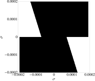
Figure 5: The basins of attraction in the $\left(\sigma,\dot{\sigma}\right)$ plane for the closed FRW model. The slice is through $a=0.9$ and $\dot{a}$ is fixed by the Hamiltonian constraint. We chose the parameters $\lambda=16$ and $E_{0}=0.499\,999\,997\,5$. The black regions correspond to collapse and the white regions inflation.

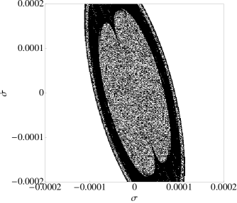
Figure 6: The basins of attraction in the $\left(\sigma,\dot{\sigma}\right)$ plane for the axisymmetric Bianchi IX model. The slice is through $a=b=0.9$, $\dot{a}=0.051\,818\,772\,5$, and $\dot{b}$ is fixed by the Hamiltonian constraint. The other parameters are the same as in Fig. 5.

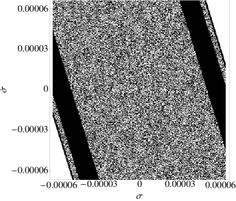
Figure 7: A magnified view of Fig. 6.

We now proceed to find a set of initial values that lead to an orbit approaching the de Sitter attractor. Such a set is called a basin of attraction. Here we use the standard method and do a pixel-by-pixel computation of a $400\times 400$ grid. Since we are dealing with basins embedded in a six-dimensional phase space, we are forced to consider lower dimensional slices, and here we choose the $\left(\sigma,\dot{\sigma}\right)$ plane although similar fractal basins of attraction can be obtained for other slices in the phase space. As shown in Fig. 5, in the closed FRW universe, we have a sharply divided separatrix even if we have a contribution from the Gauss-Bonnet term. When the metric becomes anisotropic, the basins of attraction become highly fractal as shown in Fig. 6. A magnification of the inner region is shown in Fig. 7 and reveals self-similar fractal structure. Note that the black regions correspond to orbits that collapse to the big crunch and the white regions to orbits that expand to the de Sitter space.

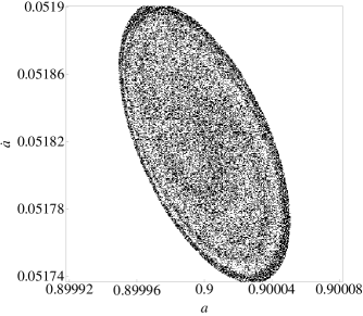
Figure 8: The basins of attraction in the $\left(a,\dot{a}\right)$ plane.

The existence of fractal structures is not restricted to one particular plane and can be seen in other slices in the six-dimensional phase space. Fig. 8 shows that similar fractal structures can also be seen in the $\left(a,\dot{a}\right)$ plane for universes with parameters and conditions identical to those used in Fig. 6. These fractal structures in the phase space cannot be removed by coordinate transformation and thus provide invariant characterization of chaos in our model.

VI Final Remarks

In this paper, we have studied the dynamics of the closed FRW models and Bianchi type-IX models in a “string-inspired” modified gravity, which may provide a description of pre-inflationary stages of the Universe after the Planck era. Higher curvature terms arise as the next-to leading terms in the superstring effective action, or from the renormalization of the stress tensor. We have included such effects in the form of a Gauss-Bonnet curvature term non-minimally coupled to a scalar field. The main features of our model are a positive cosmological constant and a perfect fluid, which produce a saddle point in the phase space. Due to the presence of the saddle point, an orbit starting in the neighborhood of the separatrix has two asymptotic possibilities, the de Sitter inflation and the big crunch collapse. In the closed FRW model, the dynamics near this critical point is reduced to simple two-dimensional hyperbolic motion of the Bogdanov-Takens bifurcation. Consequently, the closed FRW model is not chaotic. In the anisotropic Bianchi type-IX model, we restricted our attention to the axisymmetric case. The introduction of anisotropy produces unstable periodic orbits, which interact with simple hyperbolic motion of the planar Bogdanov-Takens bifurcation to produce chaotic dynamics.

Our results extend the work of de Oliveira, Soares, and Stuchi in De Oliveira et al. (1997), who describe chaotic exit to inflation for the axisymmetric Bianchi IX universe in general relativity. In subsequent papers Barguine et al. (2001); De Oliveira et al. (2002); Soares and Stuchi (2005) the authors discuss the existence of “homoclinic chaos” in general relativity. Our model does not have such homoclinic orbits because of nonlinearity due to the coupling of Gauss-Bonnet curvature and the scalar field. Furthermore, extending a cosmological model to the $a<0$ region of the phase space is physically unreasonable as pointed out in Heinzle et al. (2006).

In the model considered in De Oliveira et al. (1997), it is possible to find an energy $E_{0}$ such that a small perturbation to a point on the separatrix is a chaotic set. As we have shown in this paper, this is also true when we include a stringy correction to the Einstein-Hilbert action. We have shown that a small fluctuation in initial conditions leads to indeterminate outcome between collapse or inflation. Furthermore, we found some numerical evidence of fractal structures in the basins of attraction. The fractal basins of attraction, together with topology of cylinders near the critical point, are invariant characterization of chaos in our model.