Computation of Growth Rates and Threshold of the Electromagnetic Electron Temperature Gradient Modes in Tokamaks

Abstract

In this manuscript, eigenvalues of the Electron Temperature Gradient (ETG) modes and Ion Temperature Gradient (ITG) modes are determined numerically using Hermite and Sinc differentiation matrices based methods. It is shown that these methods are very useful for the computation of growth rates and threshold of the ETG and ITG modes. The total number of accurately computed eigenvalues for the modes have also been computed. The ideas developed here are also of relevance to other modes that use Ballooning formalism.

I Introduction

Computation of growth rates of microinstabilities in tokamaks is of considerable interest to the controlled fusion community. Often nonlocal analysis of Braginskii, Gyrokinetic or Gyrofluid equations leads us to a system of differential equations or differentio-integral equations with an unknown ’eigenvalue’. Such eigenvalue problems are encountered extensively in areas of ballooning modes, drift waves and other microinstabilities. Such equations have usually been solved by the shooting method, integral eigenvalue codes, phase integral methods and so on by a number of authors and Refs Jhowry -Raj is certainly an incomplete list.

However shooting methods suffer from a number of disadvantages. Shooting methods are very sensitive to initial conditions. It may be difficult to arrive at the right answer unless a very good approximation to the correct result is known. Furthermore, if determination the full eigenmode spectrum is intended then the whole 2-D parameter space of initial guesses $\omega_{r}+i\omega_{i}$ must be spanned. Keeping in mind sensitivity to the initial guess, this may not be easy. Shooting methods can run into difficulties if the eigenvalues of the Jacobian matrix are widely separated. Often results are determined by round off errors rather than by the equation itself. Integral eigenvalue codes like those that use methods of Delves and Lyness or Davies Method also require initial guesses Antia .

Two methods that overcome many of these disadvantages are the Finite Difference (FD) and Spectral collocation methods BoydBook . Finite difference methods consist of replacing the derivatives by an approximation ( such as $du/dx\approx[u(x+h)-u(x-h)]/2h$ where $h$ is the grid size. This introduces truncation error and accuracy may be compromised (although a finite difference method is easy to program). Higher order finite difference methods impose strong stability restriction. Gary and Hegalson gary have highlighted the usefulness of difference methods in computing eigenvalues of differential equations. Specifically, it has been pointed out by them that the shooting methods that use Muller method or Lagurre method may run into difficulties (see table VI of Ref gary ).

Spectral methods involve expansion of the solution by a finite sum in a orthogonal basis functions and minimizing of the residual BoydBook . Different spectral and pseudospectral methods differ in their minimization strategies. In this manuscript, the use of Differentiation Matrix (DM) based spectral methods to compute the ETG growth rate has been illustrated. Differentiation matrix based methods score over finite difference methods in their ease of use, greater accuracy and faster execution for the same matrix size. The importance of these methods was realized by the author through an informal comparison observed in course of this work: a $15\times 15$ DM gave similar accuracy as a $150\times 150$ FD matrix. Since computational time scales very fast (It costs $\sim 10N^{3}$ operations for the QZ Numrecipes ; QZAlg algorithm), the ratio of the time consumed in the FD method ($N=150$) while that in DM ($N=15$) would be $(150)^{3}/15^{3}=1000$!! - a huge increase in speed!. It must be noted however, the matrices involved in the DM and FD methods are, respectively, banded and full. This might make the DM method much more expensive for the same N number. Moreover, the FD performance could probably also be improved by optimizing the non-equidistant grid.

Furthermore, as will be shown in this report, ETG growth rates converge faster with differentiation matrix methods. Differentiation matrix methods have one more advantage. The process of differentiation can be done through the matrix-vector product $f^{\ell}=D^{(\ell)}f$ where $f$ is a vector of function values at the nodes $\{x_{k}\}$. For example consider the model problem

$$d^{2}f/dx^{2}-df/dx=\lambda f$$

which in matrix form becomes

$$D^{(2)}f-D^{(1)}f=\lambda f,$$

where $D^{(1)}$ and $D^{(2)}$ are a first and second order differentiation matrices respectively. Thus in these methods, the process of differentiation can be carried out through a matrix-vector product. Thus in principle one could create differentiation matrices for the curl or a gradient operator to solve more complex problems. The application of differentiation matrices is relavant to plasma physics and specifically to toroidal version of drift instabilities employing the ballooning formalism.

It must be pointed out that the goal of this manuscript is not to show that finite difference algorithms are not useful. In fact, a variety of situations can be envisaged where finite difference algorithms may be indispensible. Furthermore, neither the finite difference algorithm nor the differentiation matrix based methods used here are the very best and therefore a full academic comparison therefore cannot be done. Since a general analytical solution of the equations discussed here in not available, a comparision of numerical solutions from FD and DM methods is used as a means to fill this gap.

The main goal therefore, is to present application of differentiation matrices to linear analysis of ballooning modes. In the present paper, features of the collisionless, linear electromagnetic ETG modeTangriETG ; HortonETG are investigated used as a specific expample of ballooning type modes. The ETG mode is widely recognized as a mechanism for the small scale turbulence driven electron heat transport in tokamaks. The ETG mode is a short wavelength ($\rho_{i}>>\lambda_{\perp}>>\rho_{e}$), low frequency ($\omega<<\Omega_{e}$) fast growing mode ($\gamma_{ETG}$ $\simeq\sqrt{\epsilon_{n}\eta_{e}}c_{e}/L_{n}$) driven unstable by temperature and density gradients. Here, $\rho_{i}$ is the ion gyroradius, $\rho_{e}$ is the electron gyroradius, $\Omega_{e}$ is the electron cyclotron frequency, $\epsilon_{n}=2L_{n}/R$, $\eta_{e}=L_{n}/L_{Te}$ where $L_{n}$ is the background density scale length.

The organization of this paper is as follows. In the next section (Sec II), the basic equations of the ETG mode will be presented. An approximate solution in the strong ballooning limit is also derived and approximate eigenvectors computed (Figure 1). Finite difference and spectral collocation methods form the subject of the sections III and IV. Section III presents the finite difference method used for benchmarking. An optimised finite difference method is also presented. Next, in Sec. III, comparisons with the ’analytical approximation’ (Figure 1) is also presented. Disadvantages of the method are also highlighted. In section IV, the differentiation matrix based method are compared with the finite difference method. For this purpose, comparison is made in three different ways: (i) Growth, (ii) Matrix size, and (iii) Conjugacy of eigenvalues. Next, the problem of determination of the number of eigenvalues is addressed for which the ’nearest’ and ’ordinal’ distances have been computed. A summary and conclusions are presented in Section V.

II The basic equations of electron temperature gradient mode

In this section the fluid description of the ETG mode will be discussed and a set of basic equations will be presented. An advanced electron fluid model for the core plasma (i.e. collisionless plasma) has been used. This fluid model is analogous to the fluid equations used in Refs. (SinghNF , TangriETG , mypop ). The governing model equations are electron continuity equation, parallel momentum-equation and temperature equation:

$$\begin{array}[]{l}\omega\left[{\tau-\nabla_{\bot}^{2}}\right]\tilde{\phi}+\left[{1-\tilde{\varepsilon}_{n}(1+\tau)+(1+\eta_{e})\nabla_{\bot}^{2}}\right]k_{\theta}\tilde{\phi}\\ +\tilde{\varepsilon}_{n}k_{\theta}\tilde{T}+i\frac{{L_{n}}}{{qR}}\frac{\partial}{{\partial\theta}}(\tilde{A}_{||}k_{\bot})=0,\\ (-(\frac{\beta}{2}-\nabla_{\bot}^{2})i\omega+\frac{\beta}{2}(1+\eta_{e})ik_{\theta})\tilde{A}_{||}+\frac{{\varepsilon_{n}}}{{2q}}\frac{\partial}{{\partial\theta}}(\tilde{\phi}-\tilde{n}-\tilde{T})=0,\\ -\omega\tilde{T}+k_{\theta}\frac{5}{3}\tilde{\varepsilon}_{n}\tilde{T}+\left[{(\eta_{e}-2/3)k_{\theta}-\frac{{2\tau}}{3}\omega}\right]\tilde{\phi}=0.\\ \end{array}$$ (1)

Where $\tilde{n}$, $\tilde{\phi},\tilde{T}$ and $\tilde{A}_{||}$ are the normalized perturbations in density $\delta n$, potential ($\delta\phi$) , electron temperature ($\delta T_{e}$) and parallel vector potential ($eA_{||}/T_{e}$) respectively: $\left(\tilde{\phi},\tilde{n},\tilde{T},\delta\tilde{B}_{\parallel}\right)=L_{n}/\rho_{e}\left(e\delta\phi/T_{e0},\delta n/n_{0},\delta T_{e}/T_{e0},\delta B_{\parallel}/B\right)$, $\tilde{A}_{\parallel}=(2c_{e}L_{n}/\beta_{e}c\rho_{e})eA_{\parallel}/T_{e0}$. The perpendicular scales are normalized to $\rho_{e}$, the electron larmor radius while the parallel scale is normalized to $L_{n}$. As in the standard ballooning formalism, $\nabla_{\perp}^{2}f=-k_{\perp}^{2}f=-k_{\theta}^{2}f\left(1+(s\hat{\theta}-\alpha\sin\hat{\theta})^{2}\right),\tilde{\epsilon}_{n}=\epsilon_{n}\left[\cos\theta+\left(s\theta-\alpha\sin\theta\right)\sin\theta\right]$, $\nabla_{\parallel}f=ik_{\parallel}f\simeq\left(1/qR\right)\left(\partial f/\partial\theta\right)$ where $\theta$ is the extended coordinate in the ballooning formalism. Here $\omega$ is the unknown, complex eigenvalue to be determined and $\epsilon_{n}=2L_{n}/R$, where $R$ is the major radius and $L_{n}$ is the density scale length. Also note that this is a set of coupled, complex, differential and algebraic equations.

First, an approximate analytical solution for a qualitative comparison is presented. A general analytical solution of Eq. 1 is not available, however the most important case where one can obtain an analytical solution is the strong ballooning limit. In the strong ballooning limit, one can assume that $g(\theta)=cos(\theta)+(s\theta-\alpha sin(\theta))^{2}$ is slowly varying with $\theta$ so that $g(\theta)\simeq g(0)=1$. In this limit, Eq. 1 can be written as

$$A\frac{\partial^{2}\tilde{\Phi}}{\partial\theta^{2}}=(B+C\theta^{2})\tilde{\Phi}$$ (2)

$$A=\frac{\epsilon^{2}_{n}}{4q^{2}\hat{\omega}}\left[\left(\eta_{e}-\frac{2}{3}\right)k+\frac{5}{3}(1+\tau^{*}_{0})\epsilon_{n}\ k-\left(1+\frac{5}{3}\tau_{0}^{*}\right)\hat{\omega}\right]$$ (3)

$$B=\hat{\omega}^{2}\left(\tau_{0}^{*}+k^{2}\right)+\hat{\omega}\ k\left[1-\epsilon_{n}\left(1+\frac{10}{3}\tau^{*}_{0}\right)-k^{2}\left(1+\eta_{e}+\frac{5}{3}\epsilon_{n}\right)\right]$$

$$+\epsilon_{n}k^{2}\left[\eta_{e}-\frac{7}{3}+\frac{5}{3}\epsilon_{n}(1+\tau^{*}_{0})+\frac{5}{3}k^{2}(1+\eta_{e})\right]$$ (4)

$$C=k^{2}\hat{s}^{2}\left[\hat{\omega}^{2}-\hat{\omega}k\left(1+\eta_{e}+\frac{5}{3}\epsilon_{n}\right)+\frac{5}{3}\epsilon_{n}k^{2}(1+\eta_{e})\right]$$ (5)

where $\tau^{*}_{0}=k^{2}_{\theta}\lambda^{2}_{De}+\tau+\delta,\,\hat{\omega}=\omega L_{n}/c_{e}$ and $k=k_{\theta}\rho_{e}$. One specially looks the solutions of Eq. 2 of the form

$$\Phi(\theta)=\exp(-\sigma\theta^{2}/2),$$ (6)

where $Re(\sigma)>0$, where $\sigma=\pm\sqrt{C/A}$, this gives us the dispersion relation

$$B=-\sigma A.$$ (7)

Here $A,B$ and $C$ are parameters independent of $\theta$ as in Ref mypop . Note that the solutions of the form $\Phi(\theta)\propto F(\theta)exp(-\sigma\theta^{2})$ were used. Especially the case $F(\theta)=1$, which corresponds to the above solution.

Next, a discussion of the numerical solution of the equations [3-7] will be discussed. This will be used as a verification benchmark for the finite difference and differentiation matrix based methods of solution of Eqs. (1). The function $h(\hat{\omega})=B+\sigma A$ is a nonlinear function of the complex variable $\hat{\omega}=\omega_{r}+i\omega_{i}$, hence we have solved Eq. (7) by finding the roots of the function $h(\hat{\omega})$ using Muller method. In figure 1, the eigenvectors corresponding to $F(\theta)=1$ from the above ’analytical’ solution have been drawn as solid lines. The dots in this figure will form the subject of our next discussion - the finite difference method, which is discussed Sec. III. The solid squares in this figure refer to computation using the Hermite Method as descibed in Sec. IV. Please note that in this figure, for easy comparison the eigenvectors have been normalized in such way so that $Real[\Phi(\theta=0)]=1$ and $Imag[\Phi(\theta=0)]=1$ for all the methods.

III Finite Difference Methods

The basic equations solved in this manuscript, Eq. (1), can be considered as a system of first order ordinary differential equations of the form

$$\frac{dy_{i}}{dx}+\sum b_{j}(x)y_{j}=\lambda\sum a_{j}(x)y_{j}$$ (8)

Often, in the past, a number of authors have solved similar eigenvalue problems but as a single second order differential equation that involves powers of the eigenvalue $\lambda$ in the following manner:

$$a(x,\lambda)\frac{d^{2}y}{dx^{2}}=\sum b(x,\lambda)y$$ (9)

where $a(x,\lambda)$, $b(x,\lambda)$ can be nonlinear functions in $x$ but polynomial in the eigenvalue $\lambda$.

Finite difference methods are the most widely used methods to solve for eigenvalues of such ODE-eigenvalue problems. The basic ideology that we have used is highlighted in the following equations:

$$\frac{y_{k}-y_{k-1}}{x_{k}-x_{k-1}}+\sum b_{j}(\frac{1}{2}(x_{k}+x_{k-1}))(y_{k}+y_{k-1})/2$$ (10)

$$=\lambda\sum a_{j}(\frac{1}{2}(x_{k}+x_{k-1}))(y_{k}+y_{k-1})/2$$

An implementation of such finite difference methods is explained in Ref Antia . Although the method is elaborate, it has the following disadvantages. This method computes the eigenvalues by calculating the zeros of a determinant. These zeros are computed using an iterative process which in turn, requires guesses. Requirement of guess values that makes it no better than shooting methods discussed earlier. Furthermore, for efficient use, the basins of attraction of the various initial guesses must be known beforehand.

Instead of using the above code, a finite difference code has been developed to overcome the above shortcomings. This code has the following advantages not present in the above code: (i) generates the full eigenvalue spectrum simultaneously; (ii) there is an option to refine a particular eigenvalue; and (ii) for small changes in a parameter, the changes in a branch can be tracked automatically, otherwise it requires careful human intervention. Other salient feature are: (i) Can solve complex coupled differentio-algebraic equations; and (ii) arbitrary mesh (which is necessary and useful since boundary conditions are at infinity and the eigenfunction is expected to be localized).

Next, the finite difference numerical scheme used is explained in detail. First, an odd number of grid points such that $\theta=0$ is the central point $I_{o}$ is chosen. Next, allocate grid points such that $\theta(I_{o}+j)=-\theta(I_{o}-j)$. The points $\theta(I)$ need not be equally spaced but can be decided according to the problem at hand. The allocation of grid points was not optimized but chosen intuitively such that they are either (i) equally spaced; or (ii) $\theta\propto F(\theta_{1})$ where $\theta_{1}=0,\delta\theta,2\;\delta\theta,......,0.99$ is a set of equally spaced points between 0 and 0.99. The function $F(\theta_{1})$ can be any monotonically increasing function of $\theta_{1}$ like $1/(1-\theta_{1})$, $exp(c\theta_{1})$ and so on. Next one discretizes the two differential equations at half grid points and the algebraic equation at full grid points. All eigenvalues and eigenvectors can be obtained simultaneously if the resulting set of coupled algebraic equations are solved by the QZ algorithm.

In the strong ballooning limit, the full numerical computation closely follows the analytical results. In Figure 1, eigenvectors from both the analytical and numerical computations are depicted as a validation of the code. The solid lines indicate analytical result while the solid circles depict the numerical values. It must also be pointed out that in this figure, the x-axis range has been reduced (from the actual range used in the computation) to show that the eigenvectors from the analytical approximation closely follow the numerical result. The non-uniform distribution of grid points just explained is also illustrated in Figure 1 as solid dots.

This finite difference method is not without disadvantages. Eq. (1) has three equations (two ODE’s and one algebraic equation). Thus even for a modest mesh size of 150 points generates two matrices each of size $(3*150)\times(3*150)$. Investigation of the ETG mode requires variation of the basic parameters over a wide range. For example, for each value of shear parameter $\hat{s}$ and ballooning parameter $\alpha$, safety factor $q$, plasma beta $\beta$, temperature ratio $\tau$, eigenvalues for at least $200-300$ values of $\eta_{i}$ must be computed. This large number of values of $\eta_{i}$ are used to accurately compute the threshold and this increases the time taken by the computer.

IV Eigenvalues using Differentiation matrices

Differentiation matrices are novel, powerful methods of finding the eigenvalues of differential equations. These methods are very accurate. For smooth problems, convergence rates of the order of $O(e^{-cN})$ are often achieved Canuto ; Tadmor as compared to finite difference methods where the convergence rate are slower, typically ($N^{-2}$) or ($N^{-4}$).

The method employed is briefly explained below: A spectral collocation method Weid for solving differential equations that is based on weighted interpolants of the form:

$$f(x)\approx\sum_{j=1}^{N}\frac{\alpha(x)}{\alpha(x_{j})}\phi_{j}(x)f_{j},$$ (11)

has been used. The points $\{x_{j}\}_{j=1}^{N}$ is a set of distinct interpolation nodes, $\alpha(x)$ is a weight function, $f_{j}=f(x_{j})$ and the set of interpolating functions $\{\phi_{j}(x)\}_{j=1}^{N}$ satisfies $\phi_{j}(x_{k})=\delta_{jk}$. Where $\delta_{jk}$ is the Kronecker delta function. The differentiation matrix is then defined as a matrix with the entries:

$$D_{k,j}^{(\ell)}=\frac{d^{\ell}}{dx^{\ell}}[\frac{\alpha(x)}{\alpha(x_{j})}\phi_{j}(x)]_{x=x_{k}}$$ (12)

The process of differentiation can be done through the matrix-vector product $f^{\ell}=D^{(\ell)}f$ where $f$ is a vector of function values at the nodes $\{x_{k}\}$.

This manuscript, mostly uses the Hermite Collocation method. In the Hermite Collocation method, the nodes $x_{1},x_{2},x_{3},....x_{N}$ are the roots of $H_{N}(x)$, the Hermite polynomial. The weight function is the Gaussian function $\alpha(x)=exp(-x^{2}/2)$ and the interpolant is defined as

$$p_{N-1}(x)=\sum_{j=1}^{N}\frac{exp(-x^{2}/2)}{exp(-x_{j}^{2}/2)}\phi_{j}(x)f_{j},$$ (13)

where,

$$\phi_{j}(x)=\frac{H_{N}(x)}{H^{\prime}_{N}(x_{j})(x-x_{j})}.$$ (14)

It must be noted that the real line $(-\infty,\infty)$ may be mapped to itself by a change of variable $x=b\tilde{x}$, where $b$ is any positive real number. Thus the freedom offered by the parameter $b$ may be exploited to optimise the accuracy of the Hermite differencing process. Before proceeding further let us discuss the solution of Hermite differential equation itself. The solution the Hermite differential equation using a Hermite DM was performed. The errors in the first twenty five eigenvalues was found to be less than $10^{-8}$.

The application of this method to plasma physics is not new. It has been used in simulations of Vlasov equation since the sixties. Low order Hermite series ($N=2,3$) were shown to suppress numerical instabilities in a Vlasov simulation by Engelmann et al. Engel . More recently Shumer et al. have used velocity-scaled Hermite representations Schumer . In this manuscript, we employ Hermite differentiation matrices to compute eigenvalues of the ETG instability.

IV.1 Comparison with FD: Growth Rate

The eigenvalue of the ETG mode has also been computed using the following basic parameters $s=0.8,\tau=1,k_{\theta}=0.6,q=1.4,\epsilon_{n}=0.509$ and $\beta=0.01$, while $\eta_{i}$ is varied. A typical result from these simulations is depicted in Figure 2. In this figure, the results of computation from Finite difference method is shown as solid lines and that from Hermite method is shown as circles. As can be seen in the figure, the Hermite method requires only $N=16$ to achieve accuracy comparable with a Finite difference computation with $N=121$. The finite difference code uses an odd number of points $51,121$ etc. so as to have equal number of points to the left and to the right of $\theta=0$. Since the Hermite method requires only a small number of points, its is faster by orders of magnitudes. This allows greater parameter scans.

IV.2 Comparison with FD: Matrix Size

The eigenvalues of the ETG mode for different values on N using the finite difference method and Hermite spectral collocation method have also been computed. As depicted in Figure  (3), the Hermite method converges much before the two finite difference methods. In Figure  (3), two finite difference methods are illustated by solid triangles and crosses. These FD methods only differ in terms of how the mesh was optimized. Below $N=20$, the finite difference code (which is illustated by triangles) gives wrong results (i.e., $\omega_{i}\sim 0$), slowly this FD result begins to converge and a stable value is obtained only beyond $N=100$. To improve the convergence of the FD method, the mesh was optimized so that accuracy improves for $N<20$. This is shown as crosses in Figure (3). The Hermite method, however gives us an acceptable eigenvalue even for $N=10$, or $N=15$. Note that the computational time taken for an accurate computation would also be small since $N$ is small.

The rate of convergence of these three methods is illustated in Figure  (4) where the error $\delta(N)$ is plotted versus $N$. Here,

$$\delta(N)=\frac{\omega_{i}(N)-\omega_{i}^{h}(N=100)}{\omega_{i}^{h}(N=100)}$$ (15)

and $\omega_{i}^{h}(N=100)$ is the growth rate from the Hermite method at $N=100$. In this figure, $\delta(N)$ from the unoptimised finite difference method is represented using solid triangles, $\delta(N)$ from the optimised finite difference method is represented by crosses and the $\delta(N)$ from the differentiation matrix (Hermite) method is represented by solid dots. The solid line in this figure represents an error level of $1\%$ which is easily achieved by the Hermite method. The error also decreases fastest for the this method.

IV.3 Comparison with FD: Conjugacy of Growth Rates

Looking at the basic equations, one realizes that for a particular set of parameters, the maximum growth rate ($\gamma_{max}$) also has a complex conjugate $\gamma_{min}$. Mathematically, one expects that $\gamma_{max}=-\gamma_{min}$. This however may not be true in reality. Only one of the two roots may be more accurate than the other. Thus the difference between the two growth rates can be considered to be a measure of the numerical errors in computation. The parameter $\delta\gamma$ where,

$$\delta\gamma=\frac{\gamma_{max}+\gamma_{min}}{\gamma_{max}-\gamma_{min}},$$ (16)

can be considered as a measure of this error. To illustrate the competitiveness of the method, the variation of $\delta\gamma$ for various $N$, using the finite difference as well as the Hermite Method has also been computed. This is shown in Figure 5 where the triangles refer to a Hermite calculation while the dots refer to finite difference method. Values from both methods are small but the Hermite method appears to be slightly more accurate than finite difference. It is possible that the slightly smaller inaccuracies of the Hermite-case are simply due to a slightly unfavorable ordering in the matrix or round off errors. It must also be noted that this error is also smaller compared to the error in the approximation schemes.

IV.4 Number of Convergent Eigenvalues

The system of equations 1 has three equations in three variables. Increasing N, furthermore, would give us $3N$ eigenvalues. For an arbitrary N, increasing to infinity, the number of eigenvalues would also be large. All of these eigenvalues might not be good approximations to the eigenvalues of the actual differential equation. Physically one expects only a few of these should remain the same for every N. Thus it is important to ascertain the number of true eigenvalues of the differential equation at hand.

The following two situations can be envisaged: (i) the eigenvalue ’drifts’ as N increases. (ii) a new (probably spurious) eigenvalue is inserted between the two earlier ones. In order to ascertain the correct eigenvalues, Boyd et. al. have proposed a scheme Boyd for ocean tides bounded by meridians. Following this prescription, the ’ordinal’ and ’nearest neighbor’ drifts can be computed as explained below.

One computes eigenvalues using two different matrix sizes $N_{1}$ and $N_{2}$ such that $N_{1}/N_{2}>1/2$. The physically important eigenvalues include the highest growing ($\gamma_{max}>0$) and the most stable ($\gamma_{min}<0$) These modes are often complex conjugates of each other ($\gamma_{max}\sim-\gamma_{min}$) . Thus growth rate spectrum is then sorted in two different ways- ascending and descending.

The ordinal drift is defined by

$$\delta_{j,ordinal}=|\lambda_{j}^{N_{1}}-\lambda_{j}^{N_{2}}|,$$ (17)

where $\lambda_{j}^{N}$ is the imaginary part of the jth eigenvalue (after the eigenvalues have been sorted) as computed using N spectral coefficients.

While the nearest neighbor drift is given by

$$\delta_{j,nearest}=min_{k\epsilon[1,N_{2}]}|\lambda_{j}^{N_{1}}-\lambda_{k}^{N_{2}}|.$$ (18)

next, the intermodal drift is defined as follows

$$\begin{array}[]{clcr}\sigma_{j}=\left\{\begin{array}[]{clcr}|\lambda_{j}^{N_{1}}-\lambda_{j}^{N_{2}}|,&if\;j=1\\ {}\hfil\\ \frac{1}{2}\{|\lambda_{j}-\lambda_{j-1}|+|\lambda_{j+1}-\lambda_{j}|&if\;j>1,\end{array}\right.\end{array}$$ (23)

Boyd et. al. then recommend making a log/linear plot of the following ratios:

$$r_{j,ordinal}=\frac{min(|\lambda_{j}|,\sigma_{j})}{\delta_{j,ordinal}}$$ (24)

$$r_{j,nearest}=\frac{min(|\lambda_{j}|,\sigma_{j})}{\delta_{j,nearest}}$$ (25)

which must both be large for the eigenvalue computation to be accurate. Boyd et. al., illustrate for Legendre’s differential equation in Ref Boyd , Figure 4.

The ordinal and nearest distances for the ETG mode has been computed using the parameters $s=0.8,\tau=1,k_{\theta}=0.6,q=1.4,\epsilon_{n}=0.909,\beta=0.01$ in Equation [1]. The choice of parameters is not arbitrary, they have been chosen to be the same as those of Jenko et. al. Jenko . Next, the eigenvalues are sorted in two different ways- ascending and descending orders. A total of ten numerically accurate eigenvalues were found, five each for each case signifying five growing modes and five damped modes. The case of highest growing modes is illustrated in figure[6]. Such a large number of eigenvalues can be understood using the following argument. The argument is based on the results of the local and nonlocal analysis of the electron temperature gradient modes given in Ref. mypop by R. Singh et. al. The Equation 31 of Ref mypop is a third order dispersion relation retaining parallel dynamics. That is one growing, one stable and and real frequency branch. Moving to nonlocal, Equations 41-44, we realize that the dispersion relation is now a fifth order. Furthermore Eqns 41-44 assume solutions of the type $exp(-\sigma\theta^{2}/2)$ and ignores the higher branches with the form $H_{n}(\theta)exp(-\sigma\theta^{2}/2),\;n=1,2,3.....$ where $H_{n}$ is the Hermite polynomial. Higher values of n add more branches to be found numerically. Thus the possibility a large number of eigenvalues cannot be ruled out. This conclusion is not new. Gao et. al. gao have identified a series of unstable branches for the ETG mode. Similarly dong et. al. have shown six growing modes. Lee et. al [Lee ]have studied the three most unstable modes as a function of parameters.

One might also ask oneself if the number of these eigenvalues changes with physical parameters. The variation of the number of good, highest growing eigenvalues with the parameter $\epsilon_{n}$ has aslo been investigated. For large values of $\epsilon_{n}$ ($\sim 0.9$), the number of good eigenvalues is five. However on decreasing $\epsilon_{n}$, ($\sim 0.5$), the number of good eigenvalues increases and becomes seven.This is illustrated in figure 7. On a further decrease of $\epsilon_{n}$, ($\sim 0.2$), the large separation between good eigenvalues and spurious diminishes with the mode number $j$.

IV.5 The Sinc Method

The use of Sinc method to compute the eigenvalues of the ETG mode has also been investigated. The Sinc Method is usually applicable on an interval $(-\infty,\infty)$ using equidistant nodes with spacing $h$ and the nodes

$$x_{k}=(k-\frac{N+1}{2})h,\quad k=1,...,N$$ (26)

and the weight function$\alpha(x)=1$ and the interpolant

$$\phi_{j}(x)=\frac{sin[\pi(x-x_{j})/h]}{\pi(x-x_{j})/h}.$$ (27)

Like the Hermite method discussed earlier, the Sinc method also contains a free parameter $h$. The results are encouraging and represented in Figure 8. It gives a reasonably accurate growth rate for even N=3. Thus the Sinc method is very useful if one is interested only in the computation of growth rates. The real frequency for $N=3$ is wrong by about $20\%$ but rapidly improves as $N$ increases.

IV.6 Computation of the ITG growth rate

Apart from investigating the ETG mode in detail, some computations of the ITG mode using a different set of basic equations has also been attempted. The following are not a set of differentio-algebraic equations as Eq. (1), but a single second order differential equation as derived in Ref. guo :

$$\Omega\frac{d^{2}\psi}{d\theta^{2}}=h\left[(\Omega-1)A+2\epsilon_{n}g(\theta)+b\Omega\right]\psi$$ (28)

where

$$A=\frac{1+\frac{5}{3\tau}\frac{2\epsilon_{n}}{\Omega}g(\theta)}{F+\beta\frac{2\epsilon_{n}}{\Omega}g(\theta)}$$ (29)

Where $\psi$ is the eigenvector proportional to the normalized eigenvector $e\phi/T_{e}$ as in Ref guo . The parameter $\theta$ is the extended ballooning coordinate, $q$ is the safety factor and $s=(r/q)dq/dr$ is the shear parameter, $g(\theta)=cos(\theta)+s\theta sin(\theta)$ is a function which will be symbolized by $g$ from now on. The above equations can be converted into a polynomial eigenvalue problem of the form $\sum_{i=0}^{N}A_{N}\Omega^{N}X=0$ or

$$C_{3}\frac{d^{2}\psi}{d\theta^{2}}+[C_{5}(-C_{1}+C_{3}C_{4})\psi+C_{2}\frac{d^{2}\psi}{d\theta^{2}}]\Omega$$ (30)

$$+[C_{5}(-1+C_{1}+C_{2}C_{4}+C_{3}b)\psi]\Omega^{2}+\left[C_{5}(1+bC_{2})\psi\right]\Omega^{3}=0$$

where $C_{1},C_{2}...C_{5}$ are independent of $\Omega$ and are defined as follows:

$$C_{1}=\frac{10\epsilon_{n}g}{3\tau}\; \;C_{2}=1+\frac{5}{3\tau}$$ (31)

$$C_{3}=\frac{(1+\eta_{i})}{\tau}-\frac{5}{3\tau}+\beta 2\epsilon_{n}g\; \;C_{4}=2\epsilon_{n}g$$

$$C_{5}=\frac{q^{2}b_{\theta}\tau}{\epsilon_{n}^{2}}$$

The results of the numerical computation are depicted in Figure 9 where the dashed line corresponds to the growth rate and the dashed dotted line corresponds to the real frequency. The parameters used are $\epsilon_{n}=1,\eta_{i}=8,q=1,\tau=1,b_{\theta}=0.1$ and $s=1$ and the boundary condition $\psi=0$ at $x=\pm\infty$. As in the ETG case, the operator $d^{2}\psi/d\theta^{2}$ is replaced by the corresponding Hermite differentiation matrix.

V Summary and Remarks

Two methods to numerically solve for eigenvalues of the Electron Temperature Gradient (ETG) mode were presented. These methods were Hermite and Sinc methods. For verification purpose the growth rate was also computed analytically as well as numerically using finite difference methods. The advantages and disadvantages of each of these methods were also highlighted.

Although these methods seem promising they also suffer from some disadvantages. Firstly banded matrices of finite difference matrices are replaced by full matrices. Secondly the scaling parameter $b$ in the Hermite method or the spacing $h$ in the Sinc method must be adjusted for optimum results.

For computing ETG eigenvalues, spectral collocation methods were found to be more accurate, faster and more useful than finite difference methods. As another example, the eigenvalue equation for the Ion Temperature Gradient (ITG) modes was also attempted. Furthermore, recenly, these methods were also applied to the Drift Resistive Ballooning Modes (DRBM) with encouraging resultsTangriDRBM . Finally, the results presented here are quite general and can be applied to a number of other microinstabilities.

Acknowledgements

A major portion of this work had been done at Institute for Plasma Research, Bhat, Gandhinagar, India. The author is extremely thankful to Prof. Kaw and Prof. R. Singh for the guidance and useful discussions and suggestions and encouragement.

FIGURE CAPTIONS

1. FIG 1. Comparison of eigenvectors from different methods is shown. The analytical eigenvector from Eq. (6) is shown as a solid line and the numerical computation using the finite difference method as described in Sec III is shown as dots (and labeled FD in legend). The solid squares refer to computation using the Hermite Method as descibed in Sec. IV.

2. FIG 2. Real frequency $\omega_{r}$ and growth rate $\omega_{i}$ from finite difference method is compared with $\omega_{r}$ and $\omega_{i}$ from Hermite DM method. Note that Hermite Method with $N=16$ compares well with the finite difference method at $N=121$ when $\omega_{i}>0$ .

3. FIG 3. Real frequency $\omega_{r}$ and growth rate $\omega_{i}$ from the optimsed finite difference method (indicated by crosses) is comapred with the finite difference method (triangles) and the Hermite DM which is indicated by solid dots.

4. FIG 4. Numerical convergence of ETG growth rate as a function of N. Here, the error $\delta(N)\equiv[{\omega_{i}(N)-\omega_{i}^{h}(N=100)}]/{\omega_{i}^{h}(N=100)}$ is plotted versus N for three diffrent methods finite difference (triangles), the optimsed finite difference method (crosses) and the Hermite DM method (dots).

5. FIG 5. Numerical convergence of ETG growth rate is illustated through the congugacy of growth rates with the help of the ratio $\delta\gamma$ .

6. FIG 6. Ordinal and nearest distances plotted on a logarithmic scale versus mode number $j$ for the ETG mode, $\epsilon_{n}=0.9$.

7. FIG 7. Ordinal and nearest distances plotted on a logarithmic scale versus mode number j for the ETG mode, $\epsilon_{n}=0.5$.

8. FIG 8. Solution of the equations for the ETG real frequency $\omega_{r}$ and growth rate $\omega_{i}$ using Sinc Method is compared with the finite difference method. Note the small value of $N=3$ compares well with $N=121$.

9. FIG 9. Growth rate (solid line) and real frequency (dashed-dotted line) of the ITG mode as a function of $\epsilon_{n}$.

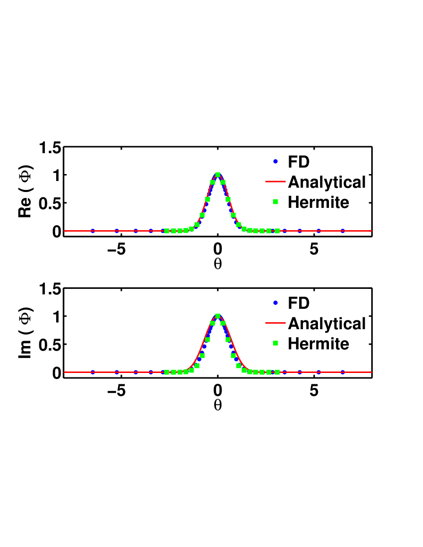
Figure 1:

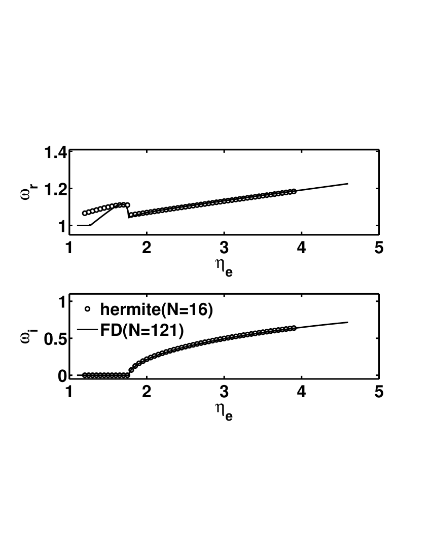
Figure 2:

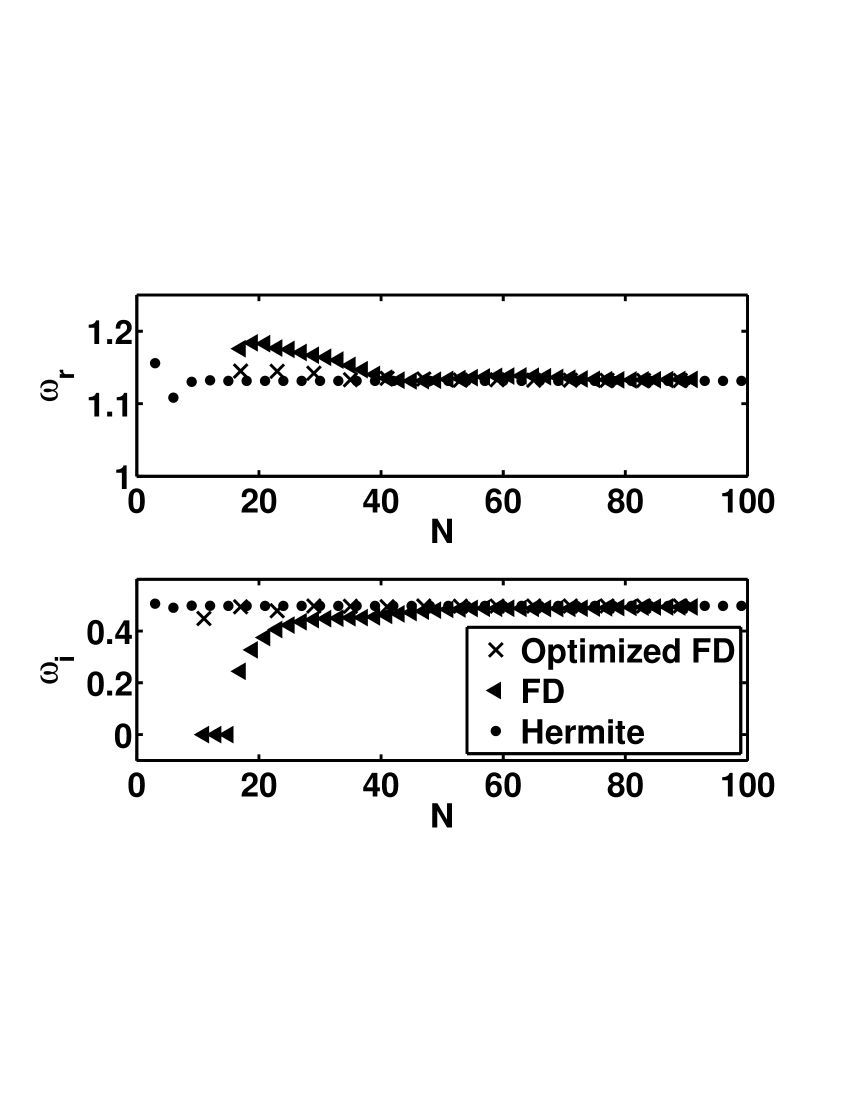
Figure 3:

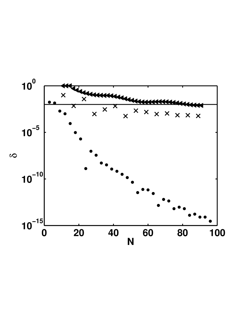
Figure 4:

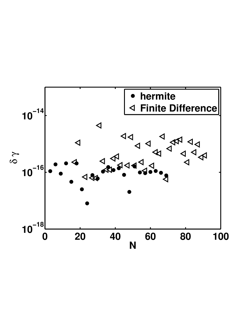
Figure 5:

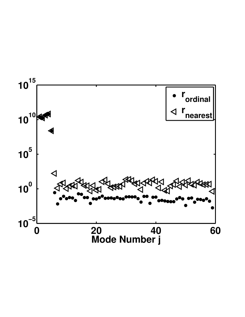
Figure 6:

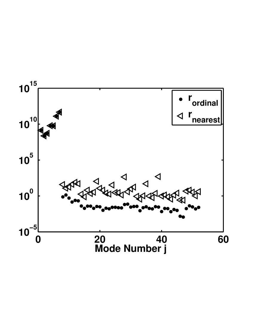
Figure 7:

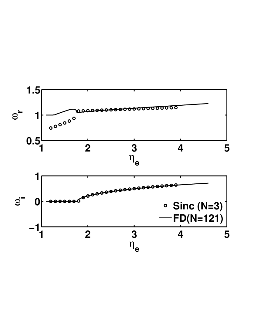
Figure 8:

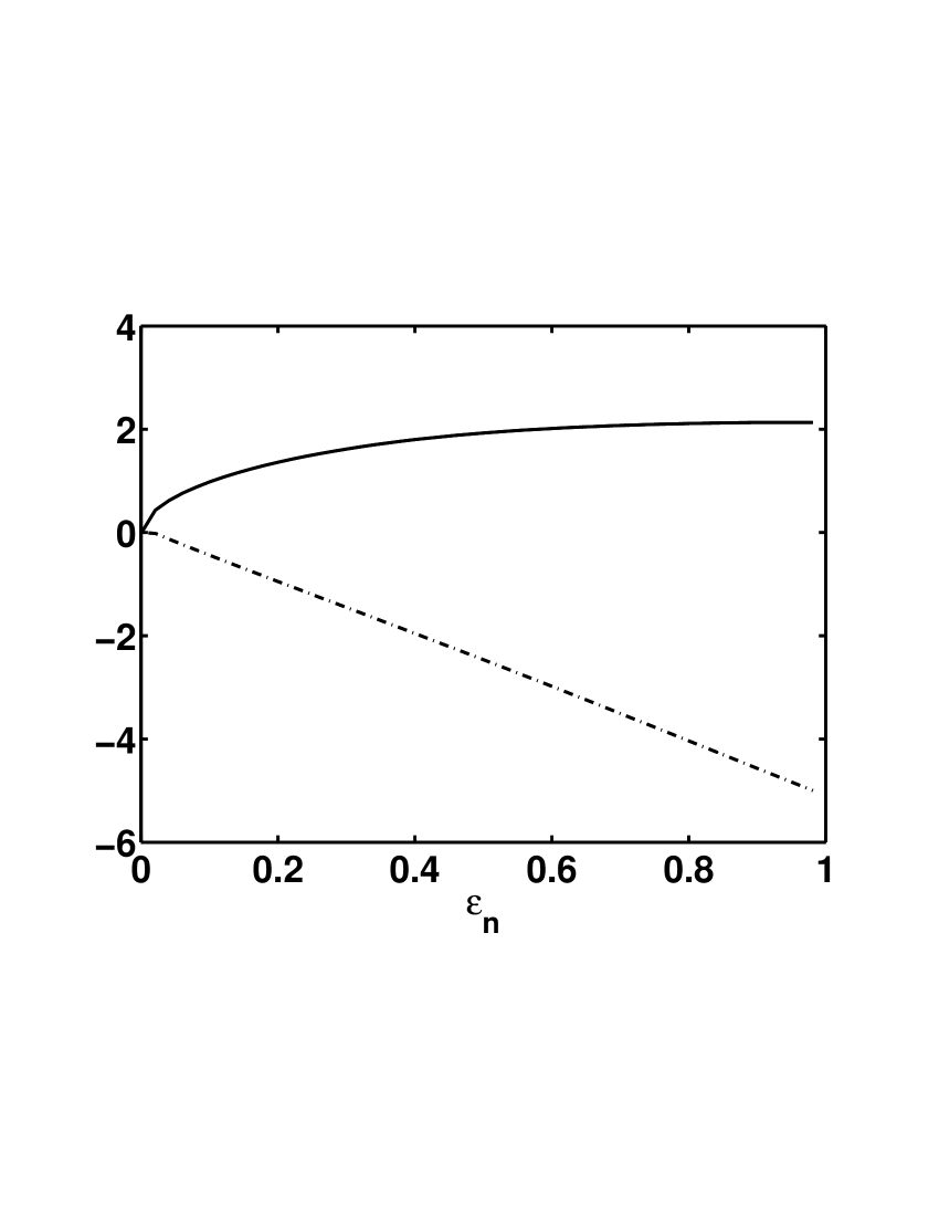
Figure 9:

References

- (1) B.Jhowry and J.Anderson Phys.Plasmas, 10, 782 (2003).
- (2) J. Anderson, H. Nordman, and J. Weiland Phys. Plasmas 8, 180 (2001).
- (3) Shozo Koshigoe and Arnold Tubis Phys. Fluids 30, 1715 (1987).
- (4) M. Yamagiwa, A. Hirose, and M. Elia Phys. Plasmas 4, 4031 (1997)
- (5) K. Rajendran, J. Q. Dong, and S. M. Mahajan Phys. Plasmas 4, 908 (1997)
- (6) J. P. Boyd J. Comput. Phys. 126 11 (1996).
- (7) C. Canuto, M. Y. Hussaini, A. Quarteroni, T. A. Zang, ’pectral Methods in Fluid Dynamics’ Springer-Verlag 1987
- (8) E. Tadmor, SIAM Journal on Numerical Analysis 23, 1 (1986).
- (9) R. Singh, P.K. Kaw and J. Weiland, Nucl. Fusion 41, 1219 (2001).
- (10) V. Tangri, R. Singh, and P. K. Kaw, Phys. Plasmas 12, 072506 (2005).
- (11) R. Singh, V. Tangri, H. Nordman, and J. Weiland et. al. Phys. Plasmas, 8, 4340 (2001).
- (12) W. Horton, B. G. Hong, and W. M. Tang, Phys. Fluids 31, 2971 (1988)
- (13) Z. Gao et. al., Phys. Plasmas, 10, 2831 (2003).
- (14) S. C. Guo and J. Weiland Nuclear Fusion, 37, 1095 (1997).
- (15) J. Q. Dong et al. Phys. Plasmas, 8, 3635 (2001).
- (16) J. A. C. Weideman and S. C. Reddy ACM Transactions on Mathematical Software Archive 26 465 (2000).
- (17) J. P. Boyd ’Chebyshev and Fourier Spectral Methods’, Dover Publications, Second Edition Pg 1.
- (18) J. W. Schumer J. Comput. Phys. 144 626 (1998).
- (19) J. Gary and R. Helgason J. Comput. Phys. 5 169 (1970).
- (20) F. Emgelmann et. al., Phys. Fluids 6 266 (1963).
- (21) H. M. Antia, Book, Tata McGraw Hill Publishers
- (22) W. H. Press , S. A. Teukolsky, W. T. Vetterling and B. P. Flannery “Numerical Recipes”, Second Edition, Cambridge Press, (2000).
- (23) C. B. Moler and G. W. Stewart, SIAM J. Numer. Anal., 10 241, (1973).
- (24) F. Jenko, W. Dorland and G. W. Hammet Phys. Plasmas, 8 4096 (2002).
- (25) Y. C. Lee, J. Q. Dong, P. N. Guzdar and C. S. Liu Phys. Fluids, 30, 1331 (1987).
- (26) V. Tangri, A. Kritz, T. Rafiq and A. Pankin, APS Annual Meeting of the APS Division of Plasma Physics, October 29–November 2 2012; Providence, Rhode Island.