Plasmon modes in the magnetically doped Single Layer and Multi layers of Helical Metals

Abstract

We study the plasmon excitations and the electromagnetic response of the magnetically doped single layer and multilayer of “helical metals”, which emerge at the surfaces of topological insulators. For the single layer case, we find a “spin-plasmon” mode with the rotating spin texture due to the combination of the spin-momentum locking of “helical metals” and the Hall response from magnetization. For the multilayers case, we investigate the electromagnetic response due to the plasmon excitations, including the Faraday rotation for the light propagating normal to the helical metal layers and an additional optical mode with the frequency within the conventional plasmon gap for the light propagating along the helical metal layers.

I Introduction

Topological insulators (TIs)Qi and Zhang (2010); Moore (2009); Hasan and Kane (2010); Qi and Zhang (2011), as a class of materials with insulating bulk states, but conducting surface states, have been theoretically proposedKane and Mele (2005a, b); Bernevig and Zhang (2006); Bernevig et al. (2006); Fu and Kane (2007); Qi et al. (2008); Moore and Balents (2007); Fu et al. (2007); Zhang et al. (2009) and experimentally realized both in two dimensions, such as HgTe quantum wellsKönig et al. (2007), and three dimensionsHsieh et al. (2008), such as Bi₂Se₃ family of materialsXia et al. (2009); Chen et al. (2009). For three dimensional (3D) TIs, for example, Bi₂Se₃, the surface state consisting of a single two dimensional (2D) Dirac cone with the gapless Dirac point protected by time reversal symmetry since the two components of the Dirac cone are Kramers’ partners. For simplicity, we can regard these two components as “spin”. The 2D surface state exhibits a novel “spin-momentum locking”Wu et al. (2006); Fu and Kane (2007); Zhang et al. (2009); Liu et al. (2010), in the sense that the “spin” is locked and points perpendicularly to the momentum, forming a left-hand helical texture in the momentum space. Therefore, the surface state of TIs is also dubbed “helical metals” (HMs)Wu et al. (2006); Raghu et al. (2010). For a finite Fermi energy $E_{f}$, the HM possesses a plasmon excitation similar to graphene with the dispersion $\sim k^{1/2}$ in the long wavelength limit (the momentum $k\rightarrow 0$). But different from graphene, this plasmon excitation is coupled to the spin wave due to the helical nature, leading to a novel “spin-plasmon” modeRaghu et al. (2010).

Another intriguing feature of a HM is the Hall response due to the lift of the degeneracy at the Dirac point by the breaking of time reversal symmetry, when the surface of TIs is coated by a ferromagnetic layer, or doped with magnetic atoms, which provide magnetization normal to the surface. If the Fermi surface lies inside the magneto-bandgap, the Hall conductance is half quantized as $e^{2}/(2h)$, known as “half quantum Hall effect”Redlich (1984); Hasan and Kane (2010); Qi and Zhang (2011); Qi et al. (2008); Fu and Kane (2007). In case of a finite Fermi surface, the Hall conductance is no longer quantized, but still non-zero. For a non-zero Hall response, the longitudinal and transverse electromagnetic self-excitations are coupled, forming a magnetoplasmon, similar to that in the conventional metals in a strong magnetic fieldAbrikosov (1988). It is interesting to ask what is the behavior of the “spin-plasmon” mode in the magnetically doped HMs.

In this paper, we investigate the interaction between electromagnetic fields and HMs on the surface of a TI with magnetic doping, focusing on the plasmon excitation. In Sec. II, we derive the correlation function for a 2D single layer of HMs and discuss how the “spin-plasmon” mode is affected by the magnetic doping. The electromagnetic waves exist in three dimensions and can not interact strongly with the 2D HMs, so we consider a model with multilayers of HMs, with an alternating stacking of TIs and normal insulators. Based on the dielectric function of this model, we discuss the propagating modes of the electromagnetic waves in HMs, in Sec. III. The conclusion is drawn in Sec. IV.

II A single-layer of Helical Metal

II.1 Correlation functions

We start from the calculation of the correlation function of a single layer of HMs on the surface($xy$ plane) of TIs with magnetic doping. The single particle HamiltonianLiu et al. (2010); Fu (2009) for this system is written by

$$\mathcal{H}_{\vec{k}}=\hbar v_{f}(\vec{k}\times\vec{\sigma})_{z}+m\sigma_{z}-E_{f}\sigma_{0}$$ (1)

where $\{\sigma_{x},\sigma_{y},\sigma_{z}\}$ are the Pauli matrices, $\sigma_{0}$ is the $2\times 2$ identity matrix and $v_{f}$ and $E_{f}$ are the Fermi velocity and Fermi energy respectively. The first term on the right hand side is the kinetic term, taking the form of Rashba spin-orbit coupling, while the second term gives the Zeeman type of coupling due to magnetization. Here we only consider the magnetization along $z$-axis for simplicity and the Zeeman coupling strength $m$ gives the gap of the HMs. The inplane current operator reads

$$\vec{\gamma}=ev_{f}(\hat{z}\times\vec{\sigma}).$$ (2)

According to the linear response theory, the current-current correlation functions read

$$\chi_{ab}(\vec{k},i\omega_{n})$$ (3)

$$= \frac{1}{\beta\mathcal{A}}\sum_{\vec{q},i\nu_{n}}\text{tr}\left[G_{0}(\vec{q},i\nu_{n})\gamma_{a}G_{0}(\vec{k}+\vec{q},i\omega_{n}+i\nu_{n})\gamma_{b}\right]$$

where $\mathcal{A}$ is the area of the surface, $a,b$ are $x$ or $y$, and $\beta$ is the inverse temperature. $G_{0}(\vec{k},i\omega_{n})$ is the single particle Matsubara’s function

$$G_{0}(\vec{k},i\omega_{n})=(i\hbar\omega_{n}-\mathcal{H}_{\vec{k}})^{-1},$$ (4)

with the Matsubara frequency $\omega_{n}$. In the long wavelength limit $k\rightarrow 0$, the rotation symmetry is restored and the correlation function is restricted to the following form

$$\chi(\vec{k},\omega)=\chi_{0}(\omega)-\chi_{H}(\omega)\sigma_{y}+o(k^{2})$$ (5)

where we only keep the momentum independent term for both the diagonal part $\chi_{0}(\omega)$ and the Hall response $\chi_{H}(\omega)$, which are calculated straightforwardly as

$$\chi_{0}(\omega)=\frac{e^{2}E_{f}}{4\pi\hbar^{2}}\left[1-\frac{x^{2}+(\frac{m}{E_{f}})^{2}}{2x}f(x)\right],$$ (6)

$$\chi_{H}(\omega)=\frac{e^{2}m}{4\pi\hbar^{2}}f(x),$$ (7)

$$f(x)\equiv\ln\left|\frac{1+x}{1-x}\right|+i\pi\theta(x-1)$$ (8)

with $x\equiv\hbar\omega/(2E_{f})$. The step function $\theta(x)$ in the imaginary part of $f(x)$ indicates the appearance of the particle-hole excitation for the frequency $\hbar\omega>2E_{f}$ in the $k=0$ limit.

Eqs. (5), (6) and (7) are the main results of this section. These expressions can recover early results in some limits. For example, without magnetization ($m=0$), the system has a longitudinal plasmon excitation with dispersion proportional to $k^{1/2}$ determined by Eq. (6), the same to the results given in Raghu et al. (2010)(see next subsection). The Hall conductance in the low frequency limit ($\omega\rightarrow 0$) can be determined by Eq. (7)

$$\sigma_{H}=\lim_{\omega\rightarrow 0}\frac{i\chi_{xy}(\omega)}{\omega}=-\frac{me^{2}}{4\pi\hbar E_{f}}$$ (9)

As $E_{f}\rightarrow m$, the system becomes insulating, and the Hall conductance tends to be $e^{2}/(2h)$, yielding the “half quantum Hall effect”Redlich (1984); Hasan and Kane (2010); Qi and Zhang (2011); Qi et al. (2008); Fu and Kane (2007).

II.2 “Spin-plasmon” modes

Now let’s consider the plasmon excitation in the presence of Hall response from Eqs. (6) and (7). Due to the existence of the Hall response, the plasmon excitation is not purely “longitudinal” anymore, but turns out to be a mixture of both the longitudinal and transverse modes. To calculate these hybrid excitations, we first note that for charges and currents distributed in a 2D sheet at $z=0$, the electric and magnetic fields in the plane can be calculated through the Coulomb’s law and Biot-Savart law

$$\vec{E}(\vec{r},t) = \int d^{2}\vec{r}^{\prime}\frac{\rho(\vec{r}^{\prime},t)(\vec{r}-\vec{r}^{\prime})}{\epsilon_{d}|\vec{r}-\vec{r}^{\prime}|^{3/2}}$$ (10)

$$B_{z}(\vec{r},t) = \frac{\mu_{d}}{c}\int d^{2}\vec{r}^{\prime}\frac{[\vec{J}(\vec{r}^{\prime},t)\times(\vec{r}-\vec{r}^{\prime})]_{z}}{|\vec{r}-\vec{r}^{\prime}|^{3/2}}$$ (11)

where $\vec{r}$, $\vec{r}^{\prime}$, $\vec{J}$ and $\vec{E}$ are all inplane vectors, and $\mu_{d}$ and $\epsilon_{d}$ are the permeability and permittivity of the surroundings respectively. Here, the magnetic field in the plane $z=0$ has only $z$ component generated by the inplane current. In Eqs. (10) and (11) we neglect the effect of retardationFetter (1973) which does not affect the key results discussed below and will be considered in the appendix.

Without loss of generality, we assume the wave is propagating along $y$ axis in the plane, so that the subscripts $x$ and $y$ correspond to the transverse and longitudinal component, respectively. In fact Eq. (10) gives the longitudinal electric field, while Eq. (11) leads to the transverse one according to the Faraday’s law $(\vec{\nabla}\times\vec{E})_{z}=-c^{-1}\partial_{t}B_{z}$. Then, after the Fourier transformation of Eq. (10) and Eq. (11), one obtains the inplane electric fields in the plane,

$$E_{x}(\vec{k},\omega) = \frac{2\pi i\mu_{d}\omega}{c^{2}k}J_{x}(\vec{k},\omega)$$ (12)

$$E_{y}(\vec{k},\omega) = -\frac{2\pi ik}{\epsilon_{d}\omega}J_{y}(\vec{k},\omega),$$ (13)

where we have applied the continuity condition $\omega\rho(\vec{k},\omega)=\vec{k}\cdot\vec{J}(\vec{k},\omega)$, to replace the charge density in Eq. (10) by the longitudinal current. Combined with Ohm’s law $\vec{J}=\sigma(\omega)\vec{E}=i(\chi/\omega)\vec{E}$, Eqs. (12) and (13) give rise to the self-consistent equation for electric fields

$$\begin{pmatrix}\chi_{0}(\omega)+\frac{c^{2}k}{2\pi\mu_{d}}&i\chi_{H}(\omega)\\ -i\chi_{H}(\omega)&\chi_{0}(\omega)-\frac{\omega^{2}\epsilon_{d}}{2\pi k}\end{pmatrix}\begin{pmatrix}E_{x}\\ E_{y}\end{pmatrix}=0.$$ (14)

Obviously, without magnetization, there is no transverse solution of the above equation, i.e., $E_{x}=0$. Only the longitudinal excitation exists with dispersion determined by

$$k=\frac{\epsilon_{d}\omega^{2}}{2\pi\chi_{0}(\omega)}.$$ (15)

In the limit $\omega\ll E_{f}$, one immediately gets the plasmon frequency $\omega=\alpha k^{1/2}$ with the coefficient $\alpha=|ev_{f}k_{f}|/(\sqrt{2\epsilon_{d}E_{f}})$, recovering the results in Raghu et al. (2010). Here $k_{f}$ is the Fermi momentum, and other quantities are defined as before. It is emphasized that the plasmon dispersion thus obtained has the divergence of group velocity as $k\rightarrow 0$, which is unphysical due to the neglecting of the effect of retardation which is rather strong for small $k$ (see the appendix)Fetter (1973).

In the presence of magnetization, the dispersion of the collective mode in HMs is determined by vanishing the determinant of the matrix in Eq. (14), which in the small $k$ limit has the following form

$$\omega(k)=\left[\frac{\left(\frac{2\pi\sigma_{H}}{\alpha\epsilon_{d}}\right)^{2}}{\alpha^{2}+\frac{c^{2}k}{\epsilon_{d}\mu_{d}}}+\frac{1}{\alpha^{2}k}\right]^{-1/2}.$$ (16)

In this case both $E_{x}$ and $E_{y}$ are nonzero, and the ratio between them is determined by

$$\frac{E_{y}}{E_{x}}=i\frac{\chi_{0}(\omega)+\frac{c^{2}k}{2\pi\mu_{d}}}{\chi_{H}(\omega)}=i\frac{\chi_{H}(\omega)}{\chi_{0}(\omega)-\frac{\omega^{2}\epsilon_{d}}{2\pi k}}.$$ (17)

It is a pure imaginary number, therefore, the electric field is not simply longitudinal but elliptically polarized in the plane of HMs for a given $\vec{k}$.

Due to the spin-orbit coupling, the collective mode in HMs can also be viewed as the spin plasmonRaghu et al. (2010). Unlike the nonmagnetized case in Ref.Raghu et al., 2010 where a simple inplane linear polarized spin density fluctuation is found, the spin density as a vector field in the magnetized case is rotating elliptically in the $xy$ plane, and the ratio between the spin densities $S_{x}$ and $S_{y}$ satisfies

$$\frac{S_{x}}{S_{y}}=-\frac{J_{y}}{J_{x}}=\frac{\omega^{2}\epsilon_{d}\mu_{d}}{c^{2}k^{2}}\frac{E_{y}}{E_{x}}$$ (18)

The spin texture $\vec{S}(\vec{r})$ in the xy plane is shown in Fig. 1

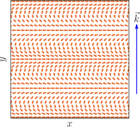
Figure 1: An illustration of spin orientation indicated by the arrows in the $xy$ plane with $S_{y}/(iS_{x})$ positive, and the wavevector $\vec{k}$ is along $y$ axis.

III Multilayers of helical metals

III.1 Dielectric functions and plasmon modes

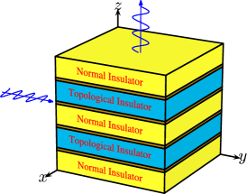
Figure 2: Illustration of layered HMs by stacking topological insulator and normal insulator alternatively. In the text, we study two basic situations of incidence, either along $y$ or $z$ axis as indicated by the blue lines.

We now consider the response of the macroscopic electromagnetic fields for layered HMs by stacking alternating layers of the TIs and normal insulators as shown in Fig. 2, with the magnetization perpendicular to HM layers.

The planes of HMs are equal spacing with the distance $l_{d}$ between adjacent layers. The local current density can be written as $\vec{J}_{loc}(\vec{k},z,\omega)=\sum_{n}\vec{J}_{n}(\vec{k},\omega)\delta(z-nl_{d})$, which is related to the local electric field by the Ohm’s law $\vec{J}_{n}(\vec{k},\omega)=(i\chi/\omega)E_{loc}(\vec{k},z=nl_{d},\omega)$ where the momentum $\vec{k}$ lies in the xy plane. The macroscopic current density and electric field in the $x,y$ direction can be obtained by averaging over the local current and local electric field, respectively,

$$\vec{\mathcal{J}}(\vec{k},z,\omega)=\int dz^{\prime}\xi(z-z^{\prime})\vec{J}_{loc}(\vec{k},z^{\prime},\omega)$$

$$\vec{\mathcal{E}}(\vec{k},z,\omega)=\int dz^{\prime}\xi(z-z^{\prime})\vec{E}_{loc}(\vec{k},z^{\prime},\omega)$$ (19)

with a test function $\xi(z-z^{\prime})$ following the standard average method for macroscopic electrodynamicsJackson (1999). We assume $l_{d}$ to be much smaller than the wavelength of the incident wave, but $l_{d}$ is still large enough so that no tunnelings occur between two adjacent layers.

Under these assumptions and using the definition of macroscopic displacement current $\partial_{t}\mathcal{D}=\partial_{t}\mathcal{E}+4\pi\mathcal{J}$ we obtain the dielectric function

$$\epsilon(\omega)=\begin{pmatrix}\epsilon_{d}-\frac{4\pi\chi_{0}(\omega)}{l_{d}\omega^{2}}&-i\frac{4\pi\chi_{H}(\omega)}{l_{d}\omega^{2}}&0\\ i\frac{4\pi\chi_{H}(\omega)}{l_{d}\omega^{2}}&\epsilon_{d}-\frac{4\pi\chi_{0}(\omega)}{l_{d}\omega^{2}}&0\\ 0&0&\epsilon_{d}\end{pmatrix},$$ (20)

where $\chi_{0}$ and $\chi_{H}$ are defined in Eq. (6) and (7). Eq. (20) immediately leads to two branches of inplane collective modes determined by $\det[\epsilon(\omega)]=0$. In the nonmagnetic case without Hall response, one obtains the familiar plasmon excitations in the normal metal in the limit $\omega\ll E_{f}$

$$\omega_{p0}^{2}=\frac{e^{2}v_{f}^{2}k_{f}^{2}}{l_{d}\epsilon_{d}E_{f}}=\frac{e^{2}v_{f}^{2}n}{\epsilon_{d}E_{f}}$$ (21)

where $n\equiv k_{f}^{2}/(4\pi l_{d})$ is the 3D electron density. Since electrons can not move in the z direction, the $E_{z}$ component of electromagnetic waves does not couple to the HMs. Eqs. (20) and (21) are obtained under the assumption that the electrons in different layers within the range of wavelength are moving in phase, since the macroscopic fields are the simple average of local ones, which is consistent with our purpose of discussing optical properties for long wavelength of electromagnetic wave. There is also another type of excitation in which the electrons in the adjacent layers moves out-of-phaseFetter (1973) and we will not consider it here. In case $m\neq 0$, the frequencies of the two branches of plasma split and are determined by

$$\omega^{2}_{p\pm}=\frac{4\pi[\chi_{0}(\omega_{p\pm})\pm\chi_{H}(\omega_{p\pm})]}{l_{d}\epsilon_{d}}.$$ (22)

The electric fields for these two plasmon modes are not oscillating linearly, but rotating clockwise and anticlockwise in the plane, respectively. These inplane plasmon excitations affect the electromagnetic wave in the bulk with inplane polarized electric fields as shown in the next section.

III.2 Electromagnetic response

Given the wavevector $\vec{k}$ in normal metal, one can distinguish the longitudinal plasmon mode ($\vec{E}\parallel\vec{k}$) from the transverse optical mode($\vec{E}\perp\vec{k}$), both of which are determined by solving the Maxwell equation

$$\left[\frac{\omega^{2}}{c^{2}}(\mu\epsilon)_{ij}-k^{2}\delta_{ij}+k_{i}k_{j}\right]E_{j}(\vec{k},\omega)=0.$$ (23)

However in the layered HMs with permittivity given in Eq. (20), the Hall response might mix the longitudinal and transverse modes, giving rise to the unusual hybrid optical modes. Since we are only interested in the influence of the collective excitations on the propagating electromagnetic wave, we consider two different situations with the inplane polarized electric field, one of which is propagating along $z$ axis, and the other is propagating in the $xy$ plane. For the electromagnetic wave with the out-of-plane polarized electric field, it is not affected by the inplane collective mode, thus will propagate in a similar way as that in a normal insulator.

III.2.1 Propagating along $z$ axis

In this case we can take $k_{x}=k_{y}=0$, $k_{z}=k$, and $E_{z}=0$, and the eigenmodes of an electromagnetic wave are simply the circularly polarized wave, $E_{y}=\mp iE_{x}$, with the minus sign for the left-hand and the plus sign for the right-hand polarization, respectively. Both modes are transverse, i.e., $\vec{E}\perp\vec{k}$, as in the normal case, but the corresponding dispersions are split as

$$\omega^{2}_{\pm}=\frac{4\pi[\chi_{0}(\omega_{\pm})\pm\chi_{H}(\omega_{\pm})]}{\epsilon_{d}l_{d}}+\frac{k^{2}c^{2}}{\epsilon_{d}\mu_{d}}.$$ (24)

due to the Hall response, as plotted in Fig. 3. There are threshhold frequencies at $k=0$ for the left-hand and right-hand modes as seen in Fig. 3, which are $\omega_{p,\pm}$ given by Eq. (22). In our parameter setting, we have $\omega_{p+}>\omega_{p-}$. Below $\omega_{p-}$, no electromagnetic wave can transmit. If $\omega_{p-}<\omega<\omega_{p+}$, only the right-hand polarized one is allowed to transmit.

Figure 3: Left panel: the dispersion for circularly polarized light propagating along $z$ axis, where we take $E_{f}=0.2eV$, $l_{d}=1000$Å, $m=0.3E_{f}$ and $\epsilon_{d}=\mu_{d}=1$. The dispersions for left-hand(blue line) and right-hand(green line) polarization split. Right panel: the angle per unit length $\kappa$ (rad/mm) is plotted as a function of $\omega$.

If $\omega>\omega_{p+}$, the Faraday rotation takes place. The Faraday rotation angle can be calculated straightforwardly as followingLandau and Lifshitz (1960)

$$\kappa(\omega)=\frac{k_{-}(\omega)-k_{+}(\omega)}{2},$$ (25)

with

$$k_{\pm}(\omega)=\frac{\omega\sqrt{\mu_{d}\epsilon_{d}}}{c}\sqrt{1-\frac{4\pi[\chi_{0}(\omega)\pm\chi_{H}(\omega)]}{\epsilon_{d}l_{d}\omega^{2}}}.$$ (26)

We plot $\kappa$ as a function of $\omega$ in the right panel of Fig. 3, where one find $\kappa$ reaches the maximum as $\omega\rightarrow\omega_{p+}$ or $\omega\rightarrow 2E_{f}/\hbar$. The giant Faraday rotation at $\omega_{p+}$ is due to the small velocity of the right-hand polarized light at its plasma frequency, while the rapid increase of the Faraday rotation angle around $\hbar\omega/(2E_{f})\sim 1$ is because the real excitation from the lower Dirac cone to the unoccupied upper Dirac cone above Fermi energy starts to happen. The Faraday rotation effect of the magnetized surface states of TIs has been carefully investigated for the insulating phaseMaciejko et al. (2010); Tse and MacDonald (2010), and here we extend the discussion to the metallic phase, which is more relevant to the present experimental situationShuvaev et al. (2011).

III.2.2 Propagating parallel to $xy$ plane

In this case, without loss of generality, we can take the incidence along $y$-axis, i.e., $k_{x}=k_{z}=0$, $k_{y}=k$, and $E_{z}=0$. The frequencies of the bulk excitations are determined by solving the following equation

$$\begin{pmatrix}1-\frac{4\pi\chi_{0}}{\epsilon_{d}l_{d}\omega^{2}}-\frac{k^{2}c^{2}}{\epsilon_{d}\mu_{d}\omega^{2}}&-i\frac{4\pi\chi_{H}}{\epsilon_{d}l_{d}\omega^{2}}\\ i\frac{4\pi\chi_{H}}{\epsilon_{d}l_{d}\omega^{2}}&1-\frac{4\pi\chi_{0}}{\epsilon_{d}l_{d}\omega^{2}}\end{pmatrix}\begin{pmatrix}E_{x}\\ E_{y}\end{pmatrix}=0\;.$$ (27)

Obviously, if there is no magnetization, i.e., $\chi_{H}=0$, the two eigenmodes are decoupled. One of them is the longitudinal plasmon excitation, and the other is the transverse mode which couples to the electromagnetic wave and determines the electromagnetic response of the medium. However in the presence of magnetization, the Hall response couples these two excitations, leading to two hybridized modes in the bulk. The dispersions of the two modes are plotted in Fig. 4, where we denote the upper branch with $\omega_{+}(k)$ and the lower one with $\omega_{-}(k)$. The lower branch, which originates from the longitudinal plasmon in the nonmagnetic case, has a dispersion and affects electromagnetic waves as well due to the mixing with the transverse mode by the Hall response.

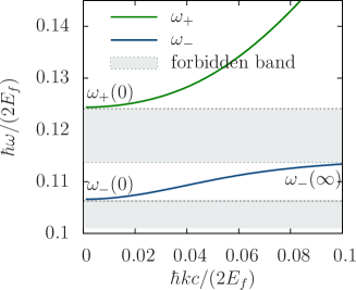
Figure 4: The dispersion of the two modes of non-transverse wave with $E_{f}=0.2eV$, $m=0.5E_{f}$, $l_{d}=1000$Å, and $\epsilon_{d}=\mu_{d}=1$.

In Fig. 4, one finds two forbidden bands for the transmission of the electromagnetic wave, which fall into the regimes $[0,\omega_{-}(0)]$ and $[\omega_{-}(\infty),\omega_{+}(0)]$, where $\omega_{-}(\infty)$ can be identified with the plasmon frequency $\omega_{p0}$ given by Eq. (21) in the nonmagnetic case, while $\omega_{\pm}(0)$ can be identified with $\omega_{p\pm}$ as given in Eq. (22). In the small $\omega$ limit, these threshold frequencies have the following form

$$\omega_{\pm}(0)=\sqrt{\left(\frac{2\pi\sigma_{H}}{l_{d}\epsilon_{d}}\right)^{2}+\omega_{p,0}^{2}}\pm\frac{2\pi|\sigma_{H}|}{l_{d}\epsilon_{d}}.$$ (28)

Similar to the single layer case, the electric field is neither perpendicular nor parallel to the wave vectors, instead, it is elliptically polarized in the $xy$ plane, as shown in the inset of the left panel of Fig. 5, where we also plot $E_{y}/(iE_{x})$ as a function of $\vec{k}$ which is determined by Eq. (27)

$$\frac{E_{y}}{iE_{x}}=\frac{4\pi\chi_{H}}{4\pi\chi_{0}-\epsilon_{d}l_{d}\omega^{2}}.$$ (29)

One can find the wave is circularly polarized at $k=0$ where $|E_{x}|=|E_{y}|$, and as $k$ increases, the wave is elliptically polarized. The upper and lower branches have opposite helicity, and $|E_{x}|>|E_{y}|$ for upper branch and $|E_{x}|<|E_{y}|$ for lower branch.

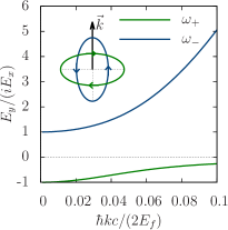
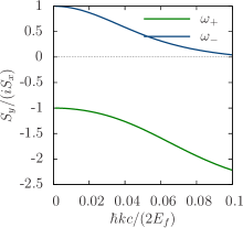
Figure 5: The ratio $E_{y}/(iE_{x})$ (left panel) and $S_{y}/(iS_{x})$(right panel) of the inplane elliptic polarization of electric fields of the propagating wave with $E_{f}=0.2eV$, $l_{d}=1000$Å, $m=0.3E_{f}$ and $\epsilon_{d}=\mu_{d}=1$. The wavevector $\vec{k}$ is along the $y$ axis. The inset of left panel gives the two inplane elliptical rotation modes of the electric fields.

One can now calculate the current accompanied with the electric field $\vec{E}$, which can be obtained from Ohm’s law and Eq. (27)

$$\begin{pmatrix}J_{x}\\ J_{y}\end{pmatrix}=\sigma(\omega)\begin{pmatrix}E_{x}\\ E_{y}\end{pmatrix}=\frac{\omega\epsilon_{d}}{4\pi i}\begin{pmatrix}\left(\frac{k^{2}c^{2}}{\mu_{d}\epsilon_{d}\omega^{2}}-1\right)E_{x}\\ -E_{y}\end{pmatrix}.$$ (30)

Due to the spin-orbit coupling, the ratio between $S_{y}$ and $S_{x}$ can then be written as

$$\frac{S_{y}}{S_{x}}=-\frac{J_{x}}{J_{y}}=\left(\frac{k^{2}c^{2}}{\epsilon_{d}\mu_{d}\omega^{2}}-1\right)\frac{E_{x}}{E_{y}}$$ (31)

We plot $S_{y}/(iS_{x})$ as a function of $k$ in the right panel of Fig. 5, which is a real number. This indicates the spin orientation in space is rotating circularly at $k=0$, and elliptically when $k>0$. This is similar to the two dimensional case as shown in section II, the only difference is that we have two elliptically polarized wave here instead of one. Our calculation shows that one may create the spin wave plasmon in stacked HMs by light with appropriate frequency and incidence along the $xy$ plane.

IV Conclusion

In conclusion, the plasmon excitation and the electromagnetic response of a single layer and multilayers of HMs are carefully investigated for the case with magnetizations. We find that the “spin-plasmon” modes discussed in Ref.Raghu et al. (2010) are modified, with the corresponding electric fields, as well as the spin orientation, becoming elliptical due to the Hall response. Since a single layer of HMs can not strongly couple to a 3D electromagnetic wave, we consider the electromagnetic response of the multilayers of HMs stacked by TIs and normal insulators. For electromagnetic waves incident normal to the HM plane, we find different plasmon frequencies for the left-hand and right-hand circularly polarized waves. Therefore, for the light with the frequency between these two plasmon frequencies, only one type of circularly polarized wave can propagate along the sample. For the frequency above both the plasmon frequencies, a giant Faraday rotation is expected. For the light propagating in the HM plane, a new branch of mode appears below the conventional plasmon frequency due to the mixing between longitudinal and transverse modes. Interestingly, the polarization of these two modes are both elliptical in the helical metal plane, no longer perpendicular to the wavevector $\vec{k}$. The new optical modes are expected to be observed in an optical transmission and reflection experimentShuvaev et al. (2011); Li et al. (2012); Jenkins et al. (2012).

V ACKNOWLEDGMENT

We would like to thank X.L. Qi for the useful discussion. This work is supported by NSFC Grant No. 10904081.

Appendix A The retardation effect in the two dimensional plasmon excitation of helical metals

In this appendix, we consider the retardation effect, which has been neglected for simplicity in Eqs. (12) and (13) in the text. For this aim, one needs to solve the full Maxwell equations subject to the time-varying sources. It is then convenient to use the potentials $\varphi$ and $\vec{A}$, which satisfy the inhomogeneous wave equations

$$\left[\frac{1}{c^{\prime 2}}\frac{\partial^{2}}{\partial t^{2}}-\vec{\nabla}^{2}\right]\varphi(x,y,z,t) = \frac{4\pi}{\epsilon_{d}}\rho(x,y,t)\delta(z)$$ (32)

$$\left[\frac{1}{c^{\prime 2}}\frac{\partial^{2}}{\partial t^{2}}-\vec{\nabla}^{2}\right]\vec{A}(x,y,z,t) = \frac{4\pi\mu_{d}}{c}\vec{J}(x,y,t)\delta(z)$$ (33)

where $c^{\prime}\equiv c/\sqrt{\mu_{d}\epsilon_{d}}$, and the Lorenz gauge in dielectric material $\vec{\nabla}\cdot\vec{A}+\mu_{d}\epsilon_{d}c^{-1}\partial_{t}\varphi=0$ is adopted. Since the system is translation invariant in the $xy$ plane, both Eq. (32) and (33) can be written in the following form after Fourier transformation

$$\left[k^{2}-\partial_{z}^{2}-\frac{\omega^{2}}{c^{\prime 2}}\right]X(\vec{k},z,\omega)=f(\vec{k},\omega)\delta(z),$$ (34)

where $\vec{k}$ is the wavevector in the $xy$ plane, and $X$ and $f$ are the potential and source respectively. This equation has extended solutions propagating in the full space with the general form

$$X(\vec{k},z,\omega)=\alpha e^{ik_{z}z}+\beta e^{-ik_{z}z}-\frac{f(\vec{k},\omega)}{2k_{z}}\sin(k_{z}|z|)$$ (35)

where $k_{z}\equiv\sqrt{(\omega/c^{\prime})^{2}-\vec{k}^{2}}$, and $\alpha$ and $\beta$ are arbitrary numbers. There is also a localized solution propagating only in the $x-y$ plane which decays exponentially along the $z$ direction,

$$X(\vec{k},z,\omega)=\frac{f(\vec{k},\omega)}{2\lambda}e^{-\lambda|z|},$$ (36)

where $\lambda=\sqrt{\vec{k}^{2}-(\omega/c^{\prime})^{2}}$. In this paper we are only interested in the localized solution Eq. (36). By substituting $X$ with $\varphi$ and $\vec{A}$, and $f$ with $\rho$ and $\vec{J}$, we have

$$\varphi(\vec{k},z,\omega) = \frac{2\pi\rho(\vec{k},\omega)}{\epsilon_{d}\lambda}e^{-\lambda|z|},$$

$$\vec{A}(\vec{k},z,\omega) = \frac{2\pi\mu_{d}\vec{J}(\vec{k},\omega)}{c\lambda}e^{-\lambda|z|}$$ (37)

Then the inplane electric field($\vec{E}\equiv-\vec{\nabla}\varphi-c^{-1}\partial_{t}\vec{A}$) reads

$$\vec{E}(\vec{k},z=0,\omega) = \frac{2\pi\vec{k}}{i\epsilon_{d}\lambda}\rho(\vec{k},\omega)+\frac{2\pi i\omega\mu_{d}}{c^{2}\lambda}\vec{J}(\vec{k},\omega)$$ (38)

Now if one assumes $\vec{k}=(0,k,0)$ along the $y$ axis, keeping the lowest order terms expanded in terms of $c^{-2}$, and using the continuity condition for the currents, then one can obtain Eqs. (12) and (13).

The group velocity in the nonmagnetized case can be calculated to be proportional to $k^{1/2}$ as $k\rightarrow 0$ without considering the effect of retardation. It is then obvious that $v_{g}\propto k^{-1/2}$ which is divergent as $k\rightarrow 0$. This unphysical feature can be cured by taking the retardation effect, i.e., by using Eq. (38). In the nonmagnetized case, the longitudinal and transverse fields are decoupled. Eq. (38) indicates that the longitudinal electric field is determined by the longitudinal current

$$E_{y}(\vec{k},0,\omega)=\frac{2\pi\lambda J_{y}}{i\epsilon_{d}\omega}.$$ (39)

According to the Ohm’s law $J_{y}={i\chi_{0}}E_{y}/{\omega}$, then we require

$$\lambda=\frac{\epsilon_{d}\omega^{2}}{2\pi\chi_{0}(\omega)}$$ (40)

For small $\omega$, we can approximate $\chi_{0}(\omega)\approx\alpha^{2}\epsilon_{d}/(2\pi)$ with $\alpha$ defined in Sec. II.2. Then

$$\left(\frac{\omega}{\alpha}\right)^{2}=\frac{2k^{2}}{\left(\frac{\alpha}{c^{\prime}}\right)^{2}+\sqrt{\left(\frac{\alpha}{c^{\prime}}\right)^{4}+4k^{2}}}$$ (41)

If $k\gg\alpha/c^{\prime}$, we recover the plasmon frequency $\alpha\sqrt{k}$ in Ref.Raghu et al. (2010). As $k\rightarrow 0$ we can not neglect the effect of retardation anymore, in fact, in the opposite limit $k\ll\alpha/c^{\prime}$, we obtain $\omega\approx c^{\prime}k$.

References

- Qi and Zhang (2010) X.-L. Qi and S.-C. Zhang, Physics Today 63, 33 (2010).
- Moore (2009) J. E. Moore, Nature Phys. 5, 378 (2009).
- Hasan and Kane (2010) M. Z. Hasan and C. L. Kane, Rev. Mod. Phys. 82, 3045 (2010).
- Qi and Zhang (2011) X.-L. Qi and S.-C. Zhang, Rev. Mod. Phys. 83, 1057 (2011).
- Kane and Mele (2005a) C. L. Kane and E. J. Mele, Phys. Rev. Lett. 95, 226801 (2005a).
- Kane and Mele (2005b) C. L. Kane and E. J. Mele, Phys. Rev. Lett. 95, 146802 (2005b).
- Bernevig and Zhang (2006) B. A. Bernevig and S. C. Zhang, Phys. Rev. Lett. 96, 106802 (2006).
- Bernevig et al. (2006) B. A. Bernevig, T. L. Hughes, and S.-C. Zhang, Science 314, 1757 (2006).
- Fu and Kane (2007) L. Fu and C. L. Kane, Phys. Rev. B 76, 045302 (2007).
- Qi et al. (2008) X.-L. Qi, T. Hughes, and S.-C. Zhang, Phys. Rev. B 78, 195424 (2008).
- Moore and Balents (2007) J. E. Moore and L. Balents, Phys. Rev. B 75, 121306 (2007).
- Fu et al. (2007) L. Fu, C. L. Kane, and E. J. Mele, Phys. Rev. Lett. 98, 106803 (2007).
- Zhang et al. (2009) H. Zhang, C.-X. Liu, X.-L. Qi, X. Dai, Z. Fang, and S.-C. Zhang, Nat Phys 5, 438 (2009).
- König et al. (2007) M. König, S. Wiedmann, C. Brüne, A. d. Roth, H. Buhmann, L. W. Molenkamp, X.-L. Qi, and S.-C. Zhang, Science 318, 766 (2007).
- Hsieh et al. (2008) D. Hsieh, D. Qian, L. Wray, Y. Xia, Y. S. Hor, R. J. Cava, and M. Z. Hasan, Nature 452, 970 (2008).
- Xia et al. (2009) Y. Xia, D. Qian, D. Hsieh, L. Wray, A. Pal, H. Lin, A. Bansil, D. Grauer, Y. S. Hor, R. J. Cava, and M. Z. Hasan, Nat Phys 5, 398 (2009).
- Chen et al. (2009) Y. L. Chen, J. G. Analytis, J. H. Chu, Z. K. Liu, S.-K. Mo, X. L. Qi, H. J. Zhang, D. H. Lu, X. Dai, Z. Fang, S. C. Zhang, I. R. Fisher, Z. Hussain, and Z.-X. Shen, Science 325, 178 (2009).
- Wu et al. (2006) C. Wu, B. A. Bernevig, and S.-C. Zhang, Phys. Rev. Lett. 96, 106401 (2006).
- Liu et al. (2010) C.-X. Liu, X.-L. Qi, H. Zhang, X. Dai, Z. Fang, and S.-C. Zhang, Phys. Rev. B 82, 045122 (2010).
- Raghu et al. (2010) S. Raghu, S. B. Chung, X.-L. Qi, and S.-C. Zhang, Phys. Rev. Lett. 104, 116401 (2010).
- Redlich (1984) A. N. Redlich, Phys. Rev. D 29, 2366 (1984).
- Abrikosov (1988) A. A. Abrikosov, Fundamentals of the Theory of Metals (Elsevier Science Publishing, 1988).
- Fu (2009) L. Fu, Phys. Rev. Lett. 103, 266801 (2009).
- Fetter (1973) A. L. Fetter, Annals of Physics 81, 367 (1973).
- Jackson (1999) J. D. Jackson, Classical Electrodynamics (John Wiley&Sons, 1999).
- Landau and Lifshitz (1960) L. D. Landau and E. M. Lifshitz, Electrodynamics of Continuous Media (Pergamon Press, 1960).
- Maciejko et al. (2010) J. Maciejko, X.-L. Qi, H. D. Drew, and S.-C. Zhang, Phys. Rev. Lett. 105, 166803 (2010).
- Tse and MacDonald (2010) W.-K. Tse and A. H. MacDonald, Phys. Rev. Lett. 105, 057401 (2010).
- Shuvaev et al. (2011) A. M. Shuvaev, G. V. Astakhov, A. Pimenov, C. Brüne, H. Buhmann, and L. W. Molenkamp, Phys. Rev. Lett. 106, 107404 (2011).
- Li et al. (2012) J. Li, Z. Y. Wang, A. Tan, P.-A. Glans, E. Arenholz, C. Hwang, J. Shi, and Z. Q. Qiu, Phys. Rev. B 86, 054430 (2012).
- Jenkins et al. (2012) G. S. Jenkins, A. B. Sushkov, D. C. Schmadel, M.-H. Kim, M. Brahlek, N. Bansal, S. Oh, and H. D. Drew, Phys. Rev. B 86, 235133 (2012).