Fractionalization of minimal excitations in integer quantum Hall edge channels

Abstract

A theoretical study of the single electron coherence properties of Lorentzian and rectangular pulses is presented. By combining bosonization and the Floquet scattering approach, the effect of interactions on a periodic source of voltage pulses is computed exactly. When such excitations are injected into one of the channels of a system of two copropagating quantum Hall edge channels, they fractionalize into pulses whose charge and shape reflects the properties of interactions. We show that the dependence of fractionalization induced electron/hole pair production in the pulses amplitude contains clear signatures of the fractionalization of the individual excitations. We propose an experimental setup combining a source of Lorentzian pulses and an Hanbury Brown and Twiss interferometer to measure interaction induced electron/hole pair production and more generally to reconstruct single electron coherence of these excitations before and after their fractionalization.

I Introduction

Coherence of electrons propagating along the edge channels of a 2DEG has been demonstrated a few years ago in electronic Mach-Zehnder interferometry experimentJi et al. (2003). This breakthrough has triggered a remarkable thread of experimentalNeder et al. (2007); Roulleau et al. (2007); Roulleau et al. (2008a, b); Litvin et al. (2007) and theoretical studiesChalker et al. (2007); Levkivskyi and Sukhorukov (2008); Kovrizhin and Chalker (2009); Neuenhahn and Marquardt (2008); Neder and Marquardt (2007). Recently, the successive partitioning of single electron and single hole excitations emitted by a mesoscopic capacitorFève et al. (2007); Mahé et al. (2010) using an electronic Hanbury Brown and Twiss setupHenny et al. (1999); Oliver et al. (1999) has been demonstratedBocquillon et al. (2012). This opens the way to quantitative studies of decoherence and relaxation of single electron excitations in electronic systemsGrenier et al. (2011a).

For example, on demand single electron sourceFève et al. (2007); Leicht et al. (2011); Hohls et al. (2012) in quantum Hall edge channels or in other non-chiral systemsTalyanskii et al. (1997); Blumenthal et al. (2007); Ahlers et al. (2006); Kaestner et al. (2008); Fujiwara et al. (2008) could be used to study the problem of quasi particle relaxation originally considered by Landau in the Fermi liquid theoryLandau (1959); Pines and Nozières (1966) and recently solved non perturbatively in integer quantum Hall edge channelsDegiovanni et al. (2009). However, considering other types of coherent single electron excitations less sensitive to decoherence and simpler to generate is certainly of great interest for the field.

Levitov, Ivanov, Lee and LesovikLevitov et al. (1996); Ivanov et al. (1997), have proposed a way to generate clean current pulses carrying single to few coherent electron excitations. Elaborating over these pioneering works, Keeling, Klich and LevitovKeeling et al. (2006) have extended this to the case of fractional excitations in FQHE and Tomonaga-Luttinger liquids. Contrary to the excitations generated by the mesoscopic capacitor Fève et al. (2007), these few electron pulses are time resolved instead of being energy resolved. Moreover, pulses that carry more than an elementary charge inject a coherent wave packet of $n$ electrons. This opens the way to entangle several electrons and to probe the full counting statisticsLevitov et al. (1996) with a finite number of particlesHassler et al. (2008).

In this paper, we show that these electron pulses are very convenient probes of fractionalizationSu et al. (1979) induced by electron/electron interactions in quantum Hall edge channels. To reach this conclusion, we have studied their decoherence and relaxation due to electron/electron interactions in a system of copropagating edge channels at filling fraction $\nu=2$ recently used to study energy relaxationAltimiras et al. (2010a); Le Sueur et al. (2010); Altimiras et al. (2010b). In this system, neutral/charged mode separationBocquillon et al. leads to fractionalization of a Lorentzian pulse propagating within one of the edge channel into two components. As in the case of non chiral 1D systemsSafi et al. (1995); Pham et al. (2000); Trauzettel et al. (2004); Steinberg et al. (2008), each of the two resulting pulses carries a fraction of the charge directly related to the interaction strength.

In a recent workNeder (2012), Neder has proposed to detect a signature of fractionalization of a continuous flow of electrons in the shot noise which is known to count the number of all excitations (electrons and holes) when the pulses are partitioned at an electronic beam splitterLevitov et al. (1996); Grenier et al. (2011b); Dubois et al. . In this paper, we propose to study the phenomenon of fractionalization at the single excitation level using Lorentzian pulses and we discuss the conditions of its observability as well as the information that could be extracted from noise measurements.

The experimental setup we propose combines a Lorentzian pulse source with an electronic Hanbury Brown and Twiss (HBT) interferometer. With our design, current noise and high frequency admittance measurements could then be combined into quantitative tests of the description of fractionalization in terms of edge magnetoplasmon scattering, recently directly measured in a $\nu=2$ edge channel systemBocquillon et al. , and which plays a role in electronic relaxation in quantum Hall edge channelsDegiovanni et al. (2009, 2010); Levkivskyi and Sukhorukov (2012) as well as decoherence in MZI interferometersLevkivskyi and Sukhorukov (2008); Neuenhahn and Marquardt (2009); Kovrizhin and Chalker (2009).

In this perspective, we present predictions for the interaction induced electron/hole pair production for Lorentzian and rectangular pulses. In the case of (screened) short range interactions, we predict stroboscopic decoherence and revivals of Lorentzian and rectangular pulses as a function of copropagation length. We identify clear signatures of fractionalization in the behavior of electron/hole production as a function of the amplitude of the pulses and of the copropagation distance. Taking into account finite temperature, we show that these signatures could be observed in realistic experiments. However, in the case of long range interactions, we show that the signature of fractionalization disappears due to the dispersion of the edge magnetoplasmon eigenmodes.

This paper is structured as follows: in section II, we briefly discuss the single electron coherence generated by a periodic source of voltage pulses. Then, in section III, we show how to describe the effect of electron/electron interactions on these pulses by combining bosonization with the Floquet scattering theory. This leads us to quantitative predictions for interaction induced electron/hole pair production in section IV.

II Generating and characterizing single electron pulses

II.1 Voltage pulse generated states

Pure electronic excitations can be created into a chiral edge channel without exciting any electron/hole pair by applying suitable voltage pulses to an Ohmic contactLevitov et al. (1996); Keeling et al. (2006). Since the average current $\langle i(t)\rangle$ injected into a single chiral edge channel by a time dependent drive $V(t)$ applied to an Ohmic contact is $\langle i(t)\rangle=(e^{2}/h)V(t)$, the voltage drive must satisfy the quantization condition such that $e\int V(t)\,dt$ be a multiple of $h$: the average emitted charge $\int\langle i(t)\rangle\,dt$ is then a multiple of the elementary charge $-e$.

But this quantization condition is not sufficient: an important result by Levitov, Lee and LesovikLevitov et al. (1996) states that in order to generate a state involving pure electronic excitations, the voltage drive $V(t)$ must be a sum of elementary Lorentzian pulses carrying exactly one electron.

II.1.1 The integer charge Lorentzian pulse as a Slater determinant

Let us start by considering a single Lorentzian voltage pulse centered at time $t=0$ such that $-e\int V(t)dt=\alpha h$ where in this paragraph, $\alpha$ is a positive integer $n$:

$$V(t)=-\frac{2\alpha\hbar}{e}\,\frac{\tau_{0}}{t^{2}+\tau_{0}^{2}}$$ (1)

where $\tau_{0}$ is the duration of the pulse.

The appropriate way to characterize single electron coherence in a many body system is to consider the two particle Green’s function at a given positionGrenier et al. (2011a); Grenier et al. (2011b):

$$\mathcal{G}^{(e)}(t,t^{\prime})=\langle\psi^{\dagger}(x,t^{\prime})\psi(x,t)\rangle$$ (2)

where the bracket denotes a quantum average in the presence of the electronic sources. This function plays the same role as the first order coherence in quantum opticsGlauber (1963). This single electron coherence characterizes the electronic quantum coherence at the single particle level: in the absence of interactions, the outcoming current from an electronic Mach-Zenhder interferometer (MZI) can indeed be expressed in terms of the incoming single electron coherenceHaack et al. (2011, 2012). Exactly as in quantum opticsLvovsky and Raymer (2009), Hanbury Brown and Twiss interferometry provides a way to reconstruct the single electron coherence from current noise measurementsGrenier et al. (2011b) or, at least, to compare excitations of quantum states emitted by two different sourcesMoskalets and Büttiker (2011) via an Hong Ou Mandel type experiment.

Being submitted to this voltage drive within the Ohmic contact, each electron accumulates an electric phase which then appears in the temporal coherence properties of electrons emitted by the Ohmic contact. In the presence of a general time dependent external drive $V(t)$, the single electron coherence of electrons $\mathcal{G}^{(e)}(t,t^{\prime})$ is given by

$$\mathcal{G}^{(e)}(t,t^{\prime})=\exp{\left(\frac{ie}{\hbar}\int_{t^{\prime}}^{t}V(\tau)\,d\tau\right)}\,\mathcal{G}^{(e)}_{\mu}(t,t^{\prime})\,.$$ (3)

where $\mathcal{G}^{(e)}_{\mu}$ denotes the single electron coherence for the edge channel at chemical potential $\mu$. For the Lorentzian pulse carrying $n$ electrons, eq. (3) becomes:

$$\mathcal{G}^{(e)}(t,t^{\prime})=\left(\frac{t+i\tau_{0}}{t-i\tau_{0}}\,\frac{t^{\prime}-i\tau_{0}}{t^{\prime}+i\tau_{0}}\right)^{n}\,\mathcal{G}_{\mu}^{(e)}(t,t^{\prime})\,.$$ (4)

At zero temperature, the contribution $\Delta_{\mu}\mathcal{G}^{(e)}=\mathcal{G}^{(e)}-\mathcal{G}^{(e)}_{\mu}$ of the pulse to single electron coherence, expressed in the frequency domain, is given by:

$$v_{F}\,\Delta_{\mu}\mathcal{G}^{(e)}(\omega_{+},\omega_{-}) = 4\pi\tau_{0}\,\Theta(\omega_{+})\Theta(\omega_{-})\,e^{-(\omega_{+}+\omega_{-})\tau_{0}}$$ (5)

$$\times \sum_{k=0}^{n-1}L_{k}(2\omega_{+}\tau_{0})L_{k}(2\omega_{-}\tau_{0})$$

where $\omega_{\pm}$ are respectively conjugate to $t$ and $t^{\prime}$ and $L_{k}$ denotes the $k$th Laguerre polynomial. The vanishing of $\Delta_{\mu}\mathcal{G}^{(e)}(\omega_{+},\omega_{-})$ when either $\omega_{+}$ or $\omega_{-}$ is negative signals the absence of hole excitations in this $n$-electron Lorentzian pulse.

In fact, expression (5) is nothing but the single electron coherence for a many body state obtained by $n$ electrons in a Slater determinant built from an orthonormal family or $n$ positive energy states on top of the Fermi sea $|F_{\mu}\rangle$ at chemical potential $\mu$. More precisely, denoting by $(\varphi_{k})_{k}$ these $n$ wave functions, Wick’s theorem directly implies that the single electron coherence of the many body state

$$|\Psi_{\mu}[(\varphi_{k})_{k}]\rangle=\prod_{k=1}^{n}\psi^{\dagger}[\varphi_{k}]\,|F_{\mu}\rangle$$ (6)

obtained by adding $n$ electrons in the $n$ single particle states $\varphi_{1},\ldots,\varphi_{n}$ is given in the space domain by

$$\mathcal{G}^{(e)}(x,y)=\mathcal{G}^{(e)}_{\mu}(x,y)+\sum_{k=1}^{n}\varphi_{k}(x)\varphi_{k}(y)^{*}\,.$$ (7)

Since, for a many body state generated from $|F_{\mu}\rangle$ by the application of an external time dependent voltage drive, single electron coherence determines all the electronic correlation functions, this shows that the many body state generated by the $n$-electron pulse (1) is obtained by adding on top of the Fermi sea the $n$ normed and mutually orthogonal wavepackets which are ($0\leq k\leq n-1$):

$$\varphi_{k}^{(\tau_{0})}(\omega)=\sqrt{2\tau_{0}}\,\Theta(\omega)e^{-\omega\tau_{0}}L_{k-1}(2\omega\tau_{0})\,.$$ (8)

Consequently, the $n$-particle wavefunction describing the added electrons is a Slater determinant built from the wavefunctions $\varphi_{k}^{(\tau_{0})}$ ($1\leq k\leq n$). Let us mention that this result can also be reached by considering the algebra of operators associated with the creation of a single $\alpha=1$ Lorentzian pulse along the lines followed by Keeling, Klich and LevitovKeeling et al. (2006).

II.1.2 Floquet approach to a periodic trains of pulses

Because single shot detection of single electron excitations is not available today, we have to resort on statistical measurements to characterize these excitations. Therefore, in practice, we shall consider a periodic source delivering an infinite train of periodically spaced pulses:

$$V(t)=\sum_{m=-\infty}^{+\infty}V_{\mathrm{p}}(t-mT)$$ (9)

where $V_{\mathrm{p}}(t)$ denotes a single pulse. As discussed in Dubois et al. , a periodic source can be used to generate a train of pulses carrying a non integer charge since the amplitude of the voltage drive can be varied continuously. In this case, each pulse can no longer be viewed as obtained from the Fermi sea by adding only electron or hole excitations. On the contrary, it should be understood as a collective excitation of the electronic fluid that contains both electron and hole excitations.

Since the voltage drive (9) is $T$-periodic, the single particle coherence (3) is also $T$-periodic. Considering $V_{\mathrm{ac}}(t)=V(t)-\alpha hf/e$ the AC part of the voltage drive, the associated phase accumulated in the time interval $[0,t]$ is periodic and can thus be decomposed in a Fourier series:

$$\exp{\left(\frac{ie}{\hbar}\int_{0}^{t}V_{\mathrm{ac}}(\tau)\,d\tau\right)}=\sum_{l=-\infty}^{+\infty}C_{l}[V_{\mathrm{ac}}]\,e^{-2\pi iflt}\,.$$ (10)

As discussed in our previous workDubois et al. , the Fourier coefficients $C_{l}[V_{\mathrm{ac}}]$ are the Floquet scattering amplitudesMoskalets and Büttiker (2002); Moskalets (2011) for electrons: for $l>0$, $C_{l}[V_{\mathrm{ac}}]$ is the amplitude for a free electron to absorb $n$ photons of energy $hf$ whereas for $l<0$ it is the amplitude for a free electron to emit $n$ photons. Finally, $C_{0}[V_{\mathrm{ac}}]$ is the amplitude for the electron not to absorb nor emit any photon. Note that the probabilities for photo assisted transitions $P_{l}[V_{\mathrm{ac}}]=|C_{l}[V_{\mathrm{ac}}]|^{2}$ sum to unity: $\sum_{l}P_{l}[V_{\mathrm{ac}}]=1$.

Using these Floquet amplitudes, the single electron coherence can then be decomposed asGrenier et al. (2011b):

$$\mathcal{G}^{(e)}(t,t^{\prime})=\sum_{n=-\infty}^{+\infty}e^{-2\pi inf\bar{t}}\int\mathcal{G}_{n}^{(e)}(\omega)\,e^{-i\omega(t-t^{\prime})}\frac{d\omega}{2\pi}\,.$$ (11)

Equations (3) and (10) then lead toDubois et al. :

$$v_{F}\mathcal{G}_{n}^{(e)}(\omega)=\sum_{l=-\infty}^{+\infty}C_{n+l}[V_{\mathrm{ac}}]\,C_{l}[V_{\mathrm{ac}}]^{*}\,f_{\bar{\mu},T_{\mathrm{el}}}(\omega-(n+2l)\pi f)\,.$$ (12)

where $f_{\bar{\mu},T_{\mathrm{el}}}$ denotes the Fermi distribution at chemical potential $\bar{\mu}=\mu+\alpha hf$ and electronic temperature $T_{\mathrm{el}}$. This shift arises from the dc component of the voltage $V(t)$. Eq. (12) expresses that the single electron coherence is built by summing the photo-generated single particle coherence over all independent electrons belonging to the shifted Fermi sea.

The nature of single particle excitations contained within the pulse train can be read from the $\mathcal{G}^{(e)}$ in the frequency domain where it is a function of the two angular frequencies $\omega_{+}$ and $\omega_{-}$ respectively conjugated to $t$ and $t^{\prime}$. For a periodic source, $\mathcal{G}^{(e)}_{n}(\omega)$ defined by (11) describes the single electron coherence for $\omega_{\pm}=\omega\pm\pi nf$: the contribution of electronic excitations (with respect to $\mu=0)$ comes from $\omega\geq\pi f|n|$ whereas the contribution from hole excitations comes from $\omega\leq-\pi f|n|$. Contributions to $\mathcal{G}^{(e)}$ in the two quadrants $|\omega|<\pi f|n|$ corresponding to $\omega_{+}\omega_{-}<0$ stem from electron hole coherencesGrenier et al. (2011b) and can be shown to be responsible for a positive peak in current correlations in an Hong-Ou-Mandel collision experimentJonckheere et al. (2012).

In the frequency domain, the diagonal part $\mathcal{G}^{(e)}_{0}(\omega)$ of the single electron coherence is nothing but the electron distribution function. For a periodic train of voltage pulses, it can be expressed in terms of the photo-assisted transition probabilitiesDubois et al. :

$$f_{e}(\omega)=v_{F}\mathcal{G}_{0}^{(e)}(\omega)=\sum_{l=-\infty}^{+\infty}P_{l}[V_{\mathrm{ac}}]\,f_{\bar{\mu},T_{\mathrm{el}}}(\omega-2\pi lf)$$ (13)

As we will see in section III, eq. (12) and (13) can also be used to compute this quantity in the presence of electron-electron interactions. But before discussing interaction effects, lets us introduce the voltage drives considered in the present paper.

II.1.3 Lorentzian and rectangular pulse trains

These expressions are valid for any periodic voltage drive and, as in our recent paperDubois et al. , three examples will be considered here: the sine periodic drive and periodic trains of Lorentzian and rectangular pulses. These voltage drives are always decomposed into a dc part $V_{\mathrm{dc}}$ and an ac component. The amplitude of the ac component is directly related to the amplitude of the dc part which determines the average charge injected per period $-\alpha e$.

For the sine voltage, $V(t)=V_{\mathrm{dc}}(1-\cos{(2\pi ft)})$ where $V_{\mathrm{dc}}=-\alpha hf/e$. The photo-assisted transition amplitudes have the well known expressionTien and Gordon (1963) $C_{n}=J_{n}(\alpha)$. The resulting excess single electron coherence $\Delta\mathcal{G}^{(e)}$ in the frequency domain is depicted on graph (a) of figure 1. As expected, it is located close to the Fermi surface and includes both electron and hole contributions as well as electron/hole coherences. Note that the photo-emission and photo-absorption probabilities are equal since the sine drive is symmetric with respect to its average $V(t+T/2)+V(t)=V_{\mathrm{dc}}$. This is clearly not the case for the two other families of pulses considered here.

For each of these two families, the physics depends on two parameters: the injected charge $\alpha$ in units of $-e$ and $f\tau_{0}$ which characterizes the compacity of the pulse train, i.e. the size of each pulse compared to their spacing. The physics of well individualized pulses is best probed at low compacityDubois et al. $f\tau_{0}\ll 1$ whereas at high compacity, a shifted Fermi sea is recovered due to the Pauli exclusion principle. To illustrate this regimes, many numerical results will be presented for $f\tau_{0}=0.01$ to shed light on the physics at the level of a single pulse.

In realistic experiments, typical values of $\tau_{0}$ are of the order of 40 ps and the drive frequency is typically $f=5\ \mathrm{GHz}$ thus leading to $f\tau_{0}\simeq 0.2$. Then a 50 mK electronic temperature corresponds to $k_{B}T_{\mathrm{el}}/hf\simeq 0.2$. Reaching lower values of $\tau_{0}$ and higher frequency drives so that $k_{B}T_{\mathrm{el}}/hf$ would be more favorable at fixed $f\tau_{0}$ would require the use of optical techniquesKato et al. (2005). Consequently, when discussing the observability of fractionalization, we will choose $f\tau_{0}=0.1$, a value within reach of current technologies.

As discussed in our recent paperDubois et al. , in the low $f\tau_{0}$ regime and at zero temperature, both Lorentzian and square pulses exhibit a minimal number of electron/hole pairs for all integer values of the charge $\alpha$ carried by each pulse. This seems to be the case for arbitrary waveforms as noticed by several authorsVanević et al. (2008); Gabelli and Reulet (2012). But in the case of the Lorenztian pulses, as predicted by Levitov, Lee and LesovikLevitov et al. (1996), the the number of hole (reps. electron) excitations vanishes for positive (reps. negative) integer values of $\alpha$ whereas for all other waveforms, it presents a non zero minimum.

The difference in these behaviors reflects the presence of hole excitations for non-Lorentzian pulses for positive integer $\alpha$. Figure 1 clearly shows the difference between a Lorentzian pulse with $\alpha=1$ (graph (b)) and a rectangular pulse with the same $\alpha$ and $f\tau_{0}$ (graph (c)): the single electron coherence for the Lorentzian pulse is localized within the electron quadrant $\omega\geq\pi f|n|$ whereas, for rectangular pulses, hole excitations as well as electron-hole coherences are present.

As can be seen from (13), this can be traced back to the properties of the Floquet amplitudes $C_{l}[V_{\mathrm{ac}}]$ for $l+\alpha<0$ whose analytical expressions for a periodic train of Lorentzian and rectangular pulses are given in appendix A. These amplitudes vanish for Lorentzian pulses for positive integer $\alpha$. As expected, the expression for the single electron coherence (12) shows that when the Floquet amplitudes $C_{l}[V_{\mathrm{ac}}]$ for $l+\alpha<0$ vanish, the excess single electron coherence due to the source has non zero contributions only in the electron quadrantGrenier et al. (2011b): this reflects the purely electronic nature of the wave packets generated by the source in this case. For negative $\alpha$ the discussion goes along the same line with holes replacing the electrons.

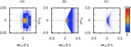
Figure 1: (Color online) Modulus of the excess single electron coherence in the frequency domain for various pulses at zero temperature and $\alpha=1$: (a) sinusoidal drive (b) Lorentzian drive $f\tau_{0}=0.01$ (c) rectangular drive with $f\tau_{0}=0.01$. Electronic (reps. hole) excitations are located in the $\omega\geq\pi|n|f$ (reps. $\omega\leq-\pi f|n|$) quadrant whereas the off diagonal $|\omega|\leq\pi f|n|$ quadrants correspond to electron/hole coherences.

II.2 Counting electron and hole pairs

II.2.1 Proposed experimental setup

Let us now describe the experimental setup that we propose to study interaction induced electron/hole pair production using shot noise measurements in an Hanbury Brown and Twiss interferometerGrenier et al. (2011b); Bocquillon et al. (2012); Dubois et al. . The setup depicted on figure 2 consists of two quantum point contacts (QPC) located at both ends of a region where two chiral edge channels interact during their copropagation. Excitations are generated by driving the Ohmic contact (1) and noise and current measurement at leads (1’) and (2’) can be performed. In a previous work, we have proposed this setup to study interchannel frequency dependent energy transfer using finite frequency noise measurementsDegiovanni et al. (2010). But as we shall now explain, playing with the polarizations of both QPCs enables us to compare electron/hole production for different propagation distances and thus to study the effects of interactions on this quantity. This idea has also been recently used to measure edge magnetoplasmon scattering in a $\nu=2$ edge channel systemBocquillon et al. .

To begin with, let us assume that the first QPC is polarized so that the inner edge channel is totally reflected and the outer one partially transmitted whereas the second QPC is unpolarized so that both channels are transmitted. This performs an HBT experiment at the first QPC in order to characterize electronic excitations propagating in the outer edge channel right for a small copropagation distance $l$.

Next, the first quantum point contact can also be polarized to inject a periodic train of single electron pulses into the outer edge channel and an equilibrium state into the inner edge channel. When the second QPC is polarized to totally reflect the inner edge channel and to partition the outer one, an HBT experiment is performed on the outer edge channel after copropagation along the inner edge channel over a large distance.

Note that in the setup proposed here, there are two easily accessible experimental controls. The first one is the amplitude of the pulse which determines the injected charge. The second one is the driving frequency of the source. In principle, one could also design a sample that allows copropagation over different distances $l$ as in the recent experiment by F. Pierre and his collaboratorsLe Sueur et al. (2010); Altimiras et al. (2010b). Combining the use of an appropriate geometry with the variation of the drive frequency keeping the compacity $f\tau_{0}$ of the source constant within the limitations of the pulse generator, one could thus explore the $(\alpha,l)$ plane and study how electron/hole pair production depends on these two parameters.

But before presenting our predictions concerning the effect of interactions, we shall now review how low frequency current noise in the HBT geometry is related to electron/hole pair production.

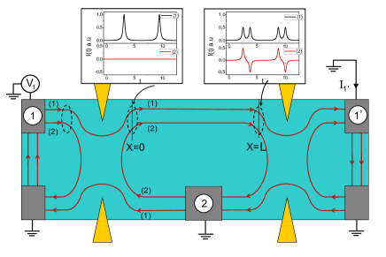
Figure 2: (Color online) Hanbury-Brown Twiss setup for the $\nu=2$ system: edge channels $(1)$ and $(2)$ interact between $x=0$ and $x=l$. The Ohmic contact $1$ is driven by the $T$-periodic voltage (9) whereas the Ohmic contact $2$ is at a fixed chemical potential. One then measures the average and the low frequency noise of the current $I_{1^{\prime}}$ at contact $1^{\prime}$. Depending on the polarizations of the two QPCs this setup performs an HBT experiment right after the source $(1^{\prime})$ or after excitations within the outer channel have co-propagated along the inner edge channel over a distance $l$.

II.2.2 Electron/hole pair production

In an HBT experiment, the current noise in one of the outcoming channels of a quantum point contact is measured at low frequency:

$$S_{1^{\prime},1^{\prime}}^{\mathrm{exp}}=\int\overline{\langle I_{1^{\prime}}(\bar{t}+\tau/2)\,I_{1^{\prime}}(\bar{t}-\tau/2)\rangle_{c}}^{\bar{t}}\,d\tau$$ (14)

where an average over $\bar{t}=(t+t^{\prime})/2$ has been taken. The outcoming current noise $S_{1^{\prime},1^{\prime}}^{\mathrm{exp}}$ contains contributions of the incoming current noise from the two incoming channel and a contribution associated with two particle interference effects. The latter can be expressed in terms of the single electron coherences of the two incoming channelsGrenier et al. (2011b). At zero temperature, when the AC drive is switched off, $S_{1^{\prime},1^{\prime}}^{\mathrm{exp}}$ is still non zero because of the partition noise of electrons due to the DC bias $V_{\mathrm{dc}}=-\alpha hf/e$. It is thus convenient to consider the excess noise $\Delta S_{1^{\prime},1^{\prime}}^{\mathrm{exp}}=(S_{1^{\prime},1^{\prime}}^{\mathrm{exp}})_{\mathrm{ac}+\mathrm{dc}}-(S_{1^{\prime},1^{\prime}}^{\mathrm{exp}})_{\mathrm{dc}}$ due to the AC part of the voltage drive: this excess noise solely arises from the partitioning of electron and hole excitations associated with the AC voltage drive. As discussed in the framework of photo-assisted noiseLesovik and Levitov (1994); Pedersen and Büttiker (1998); Rychkov et al. (2005); Schoelkopf et al. (1998); Reydellet et al. (2003); Dubois et al. and as we shall now briefly recall in the electron quantum optics language, this excess noise counts the electron/hole pair production. This procedure has originally been proposed by M. Vanevic, Y. V. Nazarov, and W. BelzigVanević et al. (2008) and discussed extensively in our previous workDubois et al. .

Since an Ohmic contact driven by an AC voltage has the same current fluctuations as in the absence of AC drive (even at non zero temperature), the excess current noise $\Delta S_{1^{\prime},1^{\prime}}^{\mathrm{exp}}$ due to the AC component of the drive voltage is given by the excess contribution arising from two particle interferences. Assuming that the QPC behaves as an energy independent electronic beam splitter with reflexion and transmission probabilities $\mathcal{R}$ and $\mathcal{T}$, $\Delta S_{1^{\prime},1^{\prime}}^{\mathrm{exp}}/\mathcal{R}\mathcal{T}$ is the overlap of the single electron and single hole excess coherences of the source due to the AC drive $\Delta\mathcal{G}_{1}^{(e/h)}(t,t^{\prime})=\mathcal{G}_{1}^{(e/h)}(t,t^{\prime})-\mathcal{G}^{(e/h)}_{\bar{\mu},T_{\mathrm{el}}}(t,t^{\prime})$ with the electron and hole coherences $\mathcal{G}^{(e/h)}_{3^{\prime}}(t,t^{\prime})$ emitted into the other incoming channelGrenier et al. (2011b):

$$\frac{\Delta S_{1^{\prime},1^{\prime}}^{\mathrm{exp}}}{\mathcal{R}\mathcal{T}}=(ev_{F})^{2}\int\overline{(\Delta\mathcal{G}^{(e)}_{1}\mathcal{G}^{(h)}_{3^{\prime}}+\Delta\mathcal{G}^{(h)}_{1}\mathcal{G}^{(e)}_{3^{\prime}})(t,t^{\prime})}^{\bar{t}}d(t-t^{\prime})\,.$$ (15)

As shown in appendix B, at vanishing temperature and for $\mu_{3^{\prime}}=\mu_{1}$ this quantity is nothing but the average excess number of excitations (electrons and holes) produced per period when the AC part of the drive is switched on. At non zero temperature, thermal electron and hole excitations in the second incoming channel antibunch with the electrons and hole excitations emitted by the source of pulses thus leading to a reduction of the noiseBocquillon et al. (2012):

$$\frac{\Delta S_{1^{\prime},1^{\prime}}^{\mathrm{exp}}}{\mathcal{R}\mathcal{T}}=\frac{e^{2}}{2\pi}\int_{-\infty}^{+\infty}\mathrm{tanh}{\left(\frac{\hbar\omega}{k_{B}T_{\mathrm{el}}}\right)}\,v_{F}\Delta\mathcal{G}^{(e)}_{1,0}(\omega)\,d\omega\,$$ (16)

where one recognizes the excess occupation number generated by the ac drive: $v_{F}\Delta\mathcal{G}^{(e)}_{1,0}(\omega)=f_{\mathrm{ac}+\mathrm{dc}}(\omega)-f_{\mathrm{dc}}(\omega)$. Note that the excess noise reduction due to the $\tanh{(\hbar\omega/k_{B}T_{\mathrm{{el}}})}$ factor concerns electron and hole excitations emitted close to the chemical potential $\mu_{1}$.

Combining (16) with the electron distribution function (13) leads to the following expression for the excess noise in terms of the photo-assisted transition probabilitiesDubois et al. :

$$\frac{\Delta S_{1^{\prime},1^{\prime}}^{(\mathrm{exp})}}{\mathcal{RT}e^{2}f} = \sum_{l=-\infty}^{+\infty}P_{l}[V_{\mathrm{ac}}]\,(l+\alpha)\coth{\left(\frac{(l+\alpha)hf}{2k_{B}T_{\mathrm{el}}}\right)}$$ (17)

$$- \alpha\coth{\left(\frac{\alpha hf}{2k_{B}T_{\mathrm{el}}}\right)}\,.$$

In the limit of vanishing temperature, the excess noise $\Delta S_{1^{\prime},1^{\prime}}^{(\mathrm{exp})}$ is given in terms of the average number of electron and holes excitations $\bar{N}_{e}$ and $\bar{N}_{h}$ emitted per period by the source:

$$\frac{\Delta S_{1^{\prime},1^{\prime}}^{\mathrm{exp}}}{\mathcal{R}\mathcal{T}} = e^{2}f\sum_{l=-\infty}^{+\infty}P_{l}[V_{\mathrm{ac}}]\,(|l+\alpha|-|\alpha|)$$ (18)

$$= e^{2}f\left((\bar{N}_{e}+\bar{N}_{h})_{T_{\mathrm{el}}=0}-|\alpha|\right)\,.$$

Our previous workDubois et al. presents a detailed study of this quantity at zero temperature for various pulse shapes and in realistic temperature conditions. In the case of Lorenztian pulses, the zero temperature excess noise vanishes when $\alpha$ is a positive (resp. negative) integer since the source then emits $\alpha$ electrons and no hole (resp. $-\alpha$ holes and no electron). For non integer values of $\alpha$, we observe a non zero electron/hole pair production as expected from the physics of orthogonality catastrophe unraveled by Levitov et alLee and Levitov ; Levitov et al. (1996).

In the next section, we will consider the effect of interactions on voltage pulses and see to what extent shot noise provides a way to study charge fractionalization. As we shall see now, expression (17) can still be used in presence of interactions provided the photo-assisted probabilities are computed from the appropriate AC voltage.

III Decoherence and relaxation

III.1 Floquet approach to decoherence for a periodic train of pulses

III.1.1 Edge magnetoplasmon scattering

To deal with interactions, it is convenient to use the bosonization framework which describes all excitations of the 1D chiral electronic fluid in terms of edge magnetoplasmon modes $b(\omega)$ and $b^{\dagger}(\omega)$ ($\omega>0$) which are directly related to the finite frequency electrical current: $i(\omega>0)=e\sqrt{\omega}\,b(\omega)$.

We then consider an interacting region where electrons within the edge channel experience electron/electron interactions or Coulomb interactions with other conductors described as a linear environment. Due to linearity, interaction effects in this region lead to an elastic scattering between the edge magnetoplasmon modes and the environmental modes. These environmental modes possibly include the edge magnetoplasmon modes of another edge channel in the case of a coupled $\nu=2$ edge channel systemDegiovanni et al. (2010) as well as the electromagnetic modes of another mesoscopic conductorDegiovanni et al. (2009). Denoting by $a(\omega)$ and $a^{\dagger}(\omega)$ where $\omega>0$ the destruction and creation operators of these modes, the effect of interactions are described by a scattering matrix $S(\omega)$ such that:

$$\left(\begin{array}[]{c}a_{\mathrm{out}}(\omega)\\ b_{\mathrm{out}}(\omega)\end{array}\right)=S(\omega)\,\left(\begin{array}[]{c}a_{\mathrm{in}}(\omega)\\ b_{\mathrm{in}}(\omega)\end{array}\right)\,.$$ (19)

As in quantum wiresSafi (1999); Safi and Schulz (1995), the magnetoplasmon scattering matrix is directly related to finite frequency admittanceDegiovanni et al. (2009, 2010): $G_{ee}(\omega)=(e^{2}/h)(1-S_{bb}(\omega))$ where $S_{bb}(\omega)$ connects $b_{\mathrm{in}}(\omega)$ to $b_{\mathrm{out}}(\omega)$.

As a consequence, it is possible to access the edge magnetoplasmon scattering amplitudes through a finite frequency admittance measurement. In the case of the setup depicted on figure 2, such measurements can be performed by polarizing the first QPC so that it reflects both edge channels or only the inner one, thus giving access to finite frequency admittance ratios. Such a measurement has recently been performedBocquillon et al. and, for the first time, has lead to direct information on edge magnetoplasmon scattering which is used to discuss electronic decoherence and relaxation in the $\nu=2$ edge channel systemLevkivskyi and Sukhorukov (2008); Degiovanni et al. (2010); Kovrizhin and Chalker (2009).

Knowing the finite frequency admittance, we can determine how interactions alter a periodic train of pulses.

III.1.2 Floquet approach and interactions

At zero temperature, a classical time dependent voltage drive $V(t)$ generates a coherent state for all magnetoplasmon modes above the shifted Fermi sea $|F_{\mu+\alpha hf}\rangle$. Introducing the notation $|[\Lambda(\omega)]\rangle$ for as coherent state characterized by the complex eigenvalues $\Lambda(\omega)$ for each $b(\omega)$ for $\omega>0$, and using the expression of the electric current in terms of $b(\omega)$ and $b^{\dagger}(\omega)$ as well as the current/voltage relation $\langle i(t)\rangle=(e^{2}/h)V(t)$, these parameters are related to the voltage drive by

$$\Lambda(\omega)=-\frac{e\widetilde{V}(\omega)}{h\sqrt{\omega}}\,$$ (20)

where $\widetilde{V}(\omega)=\int V(t)e^{i\omega t}dt$. Thus, for a periodic train of pulses, only the modes at harmonic frequencies of the driving frequency $f$ are excited. At zero temperature, the incoming state for the environmental modes is the vacuum state with respect to the environmental modes which we denote by $|[0_{\omega}]\rangle$.

Therefore, the incoming factorized state $|[\Lambda(\omega)]\rangle\otimes|[0_{\omega}]\rangle$ comes out from the interaction region as a factorized coherent state because the interaction region acts as a frequency dependent beam splitter for the edge magnetoplasmon and environmental modes. Consequently, tracing out the environmental degrees of freedom leads to a coherent state for the edge magnetoplasmon modes. This reduced state for the edge channel under consideration is of the form $|[S_{bb}(\omega)\Lambda(\omega)]\rangle$.

Therefore, the outcoming state is a pure (many-body) state generated by a distorted voltage pulse: $V_{\mathrm{out}}(\omega)=S_{bb}(\omega)V_{\mathrm{in}}(\omega)$. As a consequence, the effect of interactions on a pulse generated state can always corrected by applying an appropriate correction to the voltage pulseLebedev and Blatter (2011). In the case of a periodic train of pulses, it also implies that the outcoming single electron coherence $\mathcal{G}^{(e)}_{\mathrm{out}}$ can be computed using the Floquet approach presented in section II.1.2.

This result does indeed extend to non zero electronic temperature $T_{\mathrm{el}}$ since then, the state generated by a classical time dependent voltage drive is a displaced thermal state at temperature $T_{\mathrm{el}}$ and the environmental incoming state is the thermal equilibrium state at the temperature of the environment. As discussed in appendix C, when both temperatures are equal, the resulting outcoming state is factorized into two displaced thermal states at the common temperature. Moreover, their displacements are given by the classical scattering, exactly as in the zero temperature situation. Consequently, the outcoming single electron coherence can still be computed within the framework of Floquet scattering theoryMoskalets (2011), taking into account the non zero temperature of the electronic reservoirs.

To summarize, we have shown that the effect of interactions on a periodic train of voltage pulses can be computed exactly by combining the bosonization treatment of interactions and the Floquet formalism. We shall now apply this method to discuss the case of the system of two coupled co-propagating edge channels realized at filling fraction $\nu=2$.

First, we shall consider the simplest model for this system which assumes short range inter channel Coulomb interactions and leads to perfect spin/charge separation which in turn induces an interesting stroboscopic revival of single electron coherence. However, in a real sample, screening may not be so efficient and therefore, we shall also consider the opposite limit of long range interactions over a distance $l$ using the discrete element model originally introduced by B ttiker and his collaboratorsChristen and Büttiker (1996); Prêtre et al. (1996); Christen:1996-1. Of course the method could be adapted to other models, phenomenologicalBocquillon et al. or more microscopicHan and Thouless (1997) that include dissipation of edge magnetoplasmon modes but for simplicity we will focus on the two aforementioned models.

Finally, let us point out that the same approach could be used to discuss the effect of interactions in a system at filling fraction $\nu=1$. However, in such a system, interaction within the edge channel lead to electronic relaxation and decoherence if and only if they induce a frequency dependent time delayNeuenhahn and Marquardt (2008, 2009). This is the case as soon as we consider finite range interactions. This means that the edge magnetoplasmons of the $\nu=1$ edge channel system are dispersive and consequently that the shape of voltage voltage pulses is altered. In fact, $\nu=2$ is the first integer filling fraction which can lead to non trivial interaction effects without edge magnetoplasmon dispersion.

III.2 Stroboscopic coherence revivals

In the case of a $\nu=2$ edge channel system with short range screened Coulomb interactions, the plasmon scattering matrix associated with an interaction region of length $l$ reflects the existence of two dispersionless magnetoplasmon modes delocalized on both edges within the interaction region. It has the following formDegiovanni et al. (2010):

$$S(\omega,l)=e^{i\omega l/v_{0}}\,e^{-i\omega(l/v)(\cos{(\theta)}\sigma^{z}+\sin{(\theta)}\sigma^{x})}\,$$ (21)

where $v_{0}$ and $v$ are two velocities and $\theta$ is an angle encoding the interaction strentgh. Uncoupled channels correspond to $\theta=0$ whereas strongly coupled channels correspond to $\theta=\pi/2$. In the latter case, the eigenmodes are the symmetric and antisymmetric linear combinations of the two channel magnetoplasmon modes respectively called the charge and dipolar modesLevkivskyi and Sukhorukov (2008, 2012). The magnetoplasmon eigenmodes velocities are $v_{\pm}=v_{0}v/(v_{0}\pm v)$ and the charge mode is faster than the dipolar mode. Due to the absence of dispersion of these eigenmodes, each current pulse generated by the source splits into two pulses of the same shape and of respective weights $(1\pm\cos{(\theta)})/2$:

$$V_{1,\mathrm{out}}(t)=\frac{1+\cos{(\theta)}}{2}\,V(t-l/v_{+})+\frac{1-\cos{(\theta)}}{2}\,V(t-l/v_{-})\,.$$ (22)

This is the fractionalization of a charge $-\alpha e$ pulse. In particular, at strong coupling ($\theta=\pi/2$), we expect a single electron pulse to fractionalize into two Lorentzian pulses with $\alpha=1/2$ which can only be described in terms of collective electron/hole pair excitations.

Note that, in the case of a periodic train of pulses, an interesting phenomenon occurs when the two pulses issued from consecutive pulses recombine. When $l$ is an integer multiple of $l_{r}=vT/2$, the original current pulse is restored with a half period shift. This phenomenon can be viewed as a stroboscopic revival of the original train of excitations.

Figure 3 depicts the single electron coherence in the frequency domain at strong coupling ($\theta=\pi/2$) and for increasing propagation lengths when a periodic train of single electron pulses is injected within one edge channel. The stroboscopic revival is clearly visible as well as the appearance of hole excitations and of electron/hole coherences for propagation lengths between two revivals. Note the periodicity of the single electron coherence in $l\rightarrow l+l_{r}$ which arises from the dispersionless character of the edge magnetoplasmon eigenmodes within the interaction region, as can be seen from the explicit form of the scattering matrix (21).

In section IV, we will present predictions for the excess noise and electron/hole pair production in the $\nu=2$ edge channel system and discuss the signature of this fractionalization phenomenon both in the case of short and long range interactions.

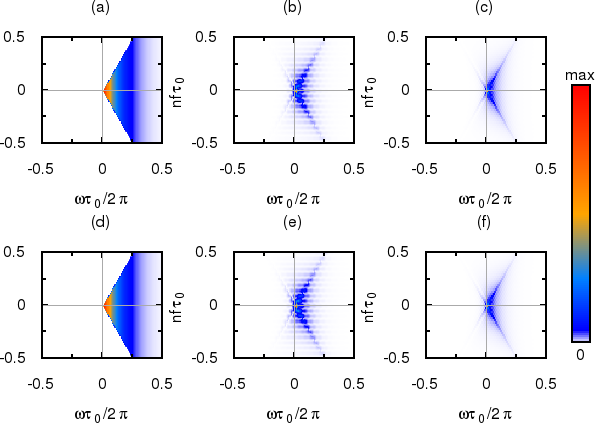
Figure 3: (Color online) Modulus of the single electron coherence function in the frequency domain emitted by a periodic source of single electron pulses ($\alpha=1$) with $\tau_{0}f=0.01$ as a function of $\omega\tau_{0}$ and $nf\tau_{0}$ in the presence of interactions at strong coupling ($\theta=\pi/2$) and for various propagation lengths: (a) $l/l_{r}=0$, (b) $l/l_{r}=0.2$, (c) $l/l_{r}=0.5$, (d) $l/l_{r}=1$, (e) $l/l_{r}=1.2$ and (f) $l/l_{r}=1.5$.

III.3 The discrete element model

To investigate the effect of long range interactions, we have used a discrete element approach to the two channel system. In this approach, pioneered by Büttiker and his collaboratorsChristen and Büttiker (1996); Prêtre et al. (1996); Christen:1996-1 , each copropagating edge channel $j$ within the interacting region $0\leq x\leq l$ experiences a uniform time dependent potential $U_{j}(t)$. These potentials are related to the charges stored on each edge channel within the interacting region by a $2\times 2$ capacitance matrix. This model is expected to describe the physics of the two channel system when interactions are unscreened and at low enough energy so that excitations sent into the interaction region do not feel the inhomogeneities of the electrostatic potential.

As shown in appendix D, the scattering matrix for the edge magnetoplasmons can be computed analytically by solving the equations of motions for the corresponding bosonic fields. As in the short range case, the scattering reflects the existence of eigenmodes which are linear combinations of the two edge magnetoplasmon modes. In the present case, their mixing angle $\theta$ is given by

$$\exp{(i\theta)}=\frac{\Delta C/2+i\,C}{\sqrt{C^{2}+\frac{\Delta C^{2}}{4}}}\,.$$ (23)

where $\Delta C=C_{1}-C_{2}$ denotes the difference of the diagonal terms of the capacitance matrix and $C$ is the off diagonal term representing the interchannel capacitance. Strong coupling is realized as soon as $C\gg|\Delta C|$. Long range interactions lead to dispersive propagation of these eigenmodes along a distance $l$. This has an important consequence for all voltage pulses: after some copropagation, their shape is not preserved. As we shall see now, this has important consequences on the observability of the fractionalization phenomenon in the $\nu=2$ quantum Hall edge channel.

IV Probing fractionalization through Hanbury Brown and Twiss interferometry

To study fractionalization in the $\nu=2$ edge channel system, we consider the electron/hole pair production as a function of $\alpha$ and of the copropagation distance $l$ which can be accessed via low frequency current noise measurements in the Hanbury Brown and Twiss geometry as explain in II.2.2. As we shall see now, the dependence of electron/hole production in $(\alpha,l)$ contains clear signatures of fractionalization and also qualitative features enabling to distinguish between short and long range interactions.

IV.1 Fractionalization in the $\nu=2$ edge channel system

IV.1.1 Short range interactions

For short range interactions, a Lorentzian pulse of charge $-\alpha e$ splits into two Lorentzian pulses of respective charges $-\alpha e\cos^{2}{(\theta/2)}$ and $-\alpha e\sin^{2}(\theta/2)$. When the charges of these pulses are non integer such as for $\alpha=1$ (single electron pulses), a non vanishing electron/hole pair production is expected at a generic distance (i.e. not a multiple of the revival distance $l_{r}$).

Nevertheless, electron/hole pair production does vanish when fractionalization leads to purely electronic pulses. For short range interactions, this is the case when $\alpha\cos^{2}{(\theta/2)}$ and $\alpha\sin^{2}{(\theta/2)}$ are both integers. This first implies that $\alpha$ is an integer and, consequently, that $\cos^{2}{(\theta/2)}$ is a rational number. Assuming that $\cos^{2}{(\theta/2)}=p/p^{\prime}$ where $p$ and $p^{\prime}$ are two mutually prime numbers, as soon as $\alpha$ is a multiple of $p^{\prime}$, electron/hole pair production will vanish for any co-propagation length. These lines of vanishing electron/hole pair production in the $(\alpha,l/l_{r})$ plane correspond to the fractionalization of the charge $-\alpha e$ in two integer charges and therefore we shall call them integer fractionalization lines.

The density plot of figure 4 presents the excess noise for Lorentzian pulses at zero temperature in the $(\alpha,l/l_{r})$ plane at strong coupling ($\theta=\pi/2$) and for $f\tau_{0}=0.01$. It clearly shows that the $\alpha=2$ and $\alpha=4$ Lorentzian pulses are always fractionalized into purely electronic pulses for any $l/l_{r}$. We also see that when $l/l_{r}$ is close to an integer, the excess noise also decreases for $\alpha=1$ and $\alpha=3$. At a higher value of $f\tau_{0}$, the same qualitative picture can still be observed but the peak values for the excess noise in units of $e^{2}f$ are lower, thus making it more difficult to observe. This decrease, specific to Lorentzian pulsesDubois et al. , is indeed related to the Pauli exclusion principle and reflect the fact that when $\alpha$ increases from a positive integer $n$ to $n+1/2$, the ’half-electronic’ excitation is added on top of a many-body state obtained by adding on top of the Fermi sea the $n$-particle state discussed in section II.1.1 on top of the Fermi surface. Single particle states just above the Fermi energy being more and more occupied with increasing $n$, the number of hole excitations generated decreases with $n$. Nevertheless, observing this pattern of minimas for the excess noise in the $(\alpha,l/l_{r})$ plane would be a clear signature of fractionalization in the $\nu=2$ edge channel system. Before analyzing in more detail the effect of the pulse shape and temperature which are relevant for the experiments, let us discuss the position of these fractionalization lines.

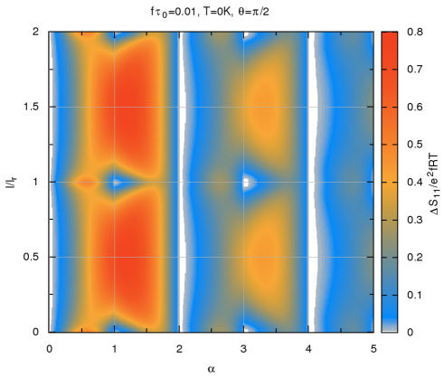
Figure 4: (Color online) Density plot representing the excess noise at zero temperature in the $(\alpha,l/l_{r})$ plane for Lorentzian pulses with $f\tau_{0}=0.01$ in the presence of short range interactions in the strong coupling regime ($\theta=\pi/2$). The integer fractionalization line at $\alpha=2$ and $\alpha=4$ are clearly visible as white vertical zones. Note also the excess noise minima (white spots) around $(\alpha,l/l_{r})=(1,n)$, $(3,n)$ for $n=0$, $1$ and $2$.

Integer fractionalization lines are determined by the interaction strength and therefore by the angle $\theta$. Figure 5 represents the hole production computed at $l=l_{r}/2$ as a function of $\theta$ for $\alpha=1$ to $\alpha=4$ Lorentzian pulses. As expected, the $\alpha=1$ pulse never leads to a vanishing electron/hole pair production as soon as $\theta\neq 0$. The $\alpha=2$ Lorentzian pulses lead to vanishing electron/hole production when it is split into two pulses of equal amplitudes: this occurs at $\theta=\pi/2$. For $\alpha=3$ Lorentzian pulse, splitting into charge $2$ and $1$ pulses occurs when $\cos{(\theta)}=\pm 1/3$. The $\alpha=4$ case leads to a vanishing of electron/hole pair production for $\theta=\pi/3$ corresponding to a splitting $4=3+1$ of the charge, and $\theta=\pi/2$ corresponding to $4=2+2$. These integer fractionalization lines are listed in table 1 for $2\leq\alpha\leq 4$. Finding these lines gives a rough estimation of $\theta$ as shown on figure 5. However, let us stress that finite frequency admittance measurementsBocquillon et al. give an independent and more precise determination of the angle $\theta$. Combining these measurements would thus provide a consistency check of our edge magnetoplasmon scattering approach to relaxation and decoherence of pulse excitations.

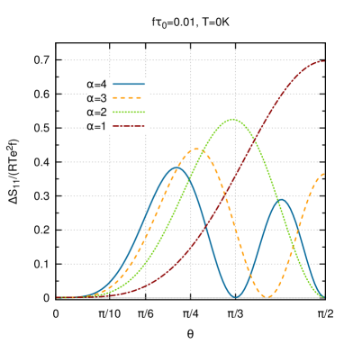
Figure 5: (Color online) Electron/hole pair production in the presence of short range interactions, observed at $l=l_{r}/2$ as a function of $\theta$ for $\alpha=1$ to $\alpha=4$ Lorentzian pulses with $f\tau_{0}=0.1$. The vanishing of excess noise for these various curves occurs at the angles listed in table 1. Note that excess noise decreases with increasing $\alpha$.

$\alpha$	$\theta$	$\cos^{2}{(\theta/2)}$	$\sin^{2}{(\theta/2)}$
$1$	$0$	$1$	$0$
$2$	$\pi/2$	$1/2$	$1/2$
$3$	$\arccos{(1/3)}$	$2/3$	$1/3$
	$\arccos{(-1/3)}$	$1/3$	$2/3$
$4$	$\pi/3$	$3/4$	$1/4$
	$\pi/2$	$2/4$	$2/4$
	$2\pi/3$	$1/4$	$3/4$

Table 1: Integer fractionalization lines for $2\leq\alpha\leq 4$ Lorentzian pulses. For each value of $\alpha$, the values of $\theta$ for which integer fractionalization of $\alpha$ pulses take place and the corresponding fractions are given.

As can be seen from figure 4, increasing $\alpha$ does not improve the observability of fractionalization as could be expected from our previous workDubois et al. : since local interactions split pulses into pulses of the same shape, we expect the effect of interaction induced fractionalization to be lower at higher $\alpha$ for Lorentzian pulses.

IV.1.2 Finite range interactions

Finite range interactions lead to the distortion of the injected pulses and therefore will affect the electron/hole pair production. A natural question is therefore to understand how finite range interactions will affect the simple physical picture discussed in the previous paragraph. Although the answer to this question is model dependent, the discrete element model provides an answer in the case of long range interactions between the two edge channels.

Figure 6 presents the zero temperature excess noise $\Delta S_{1,1}^{(\mathrm{out})}$ for Lorentzian pulses in the non interacting case compared to the predictions for the short range interaction model and for the discrete element model. As expected, we observe vanishings of the zero temperature excess noise for short range interactions whereas long range interactions leads to non vanishing minima. However, this strong quantitative difference is specific to the zero temperature case where the excess noise exactly reflects the intrinsic electron/hole pair production of the excitations present within the system. But at finite temperature, this signature of long range interactions may not be so clear.

For this reason, it is important to consider more realistic situations taking into account the finite electronic temperature as well as the non ideality of the pulses. In the forthcoming section, we will present numerical results for the excess noise taking into account finite temperature for Lorentzian and rectangular pulses with realistic parameters. First we will discuss the observability of fractionalization induced by short range interactions and next, we will consider the case of long range interactions.

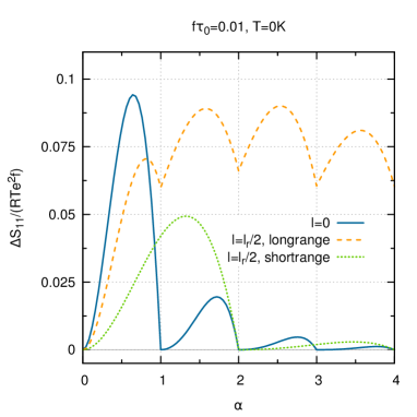
Figure 6: (Color online) Electron/hole pair production in the presence of long and short range interactions at strong coupling, observed at $l=l_{r}/2$ as a function of $\alpha$ for Lorentzian pulses with $f\tau_{0}=0.01$. The dashed curve correspond to long range interactions and shows to minima at integer values of $\alpha$ with non vanishing electron/hole pair production. The full line correspond to the non-interacting case obtained for $l/l_{r}=0$.

IV.2 Numerical results

In this section, we present numerical results for the excess noise $\Delta S_{1,1}^{(\mathrm{out})}$ in units of $e^{2}f$ obtained by applying the Floquet approach described in section III.1.2 in the short range interaction model as well as in the discrete element model. Both are considered at strong coupling ($\theta=\pi/2$), as expected from recent experimentsDegiovanni et al. (2010); Le Sueur et al. (2010); Bocquillon et al. .

We consider Lorentzian pulses with $\tau_{0}=120~{}\mathrm{ps}$ pulses at a $1.2\ \mathrm{Ghz}$ drive frequency which could be generated by state of the art arbitrary waveform generators (AWG). For rectangular pulses, we consider $\tau_{0}=40~{}\mathrm{ps}$ pulses since these can be generated with a single step by the AWG and therefore have the shortest available time step. In this case, $e^{2}f\simeq 3\times 10^{-29}\ \mathrm{A}^{2}/\mathrm{Hz}$. Our numerical results show that a sensitivity of the order of a percent of $e^{2}f$ is requested corresponding to a few $10^{-31}\ \mathrm{A}^{2}/\mathrm{Hz}$. Note that a $10^{-30}\ \mathrm{A}^{2}/\mathrm{Hz}$ sensitivity has been reached in recent experimentsParmentier et al. (2011); Bocquillon et al. (2012).

Electronic temperatures $T_{\mathrm{el}}=5$, $10$, $20$ and $40$ mK have been considered to analyze the effect of a temperature, keeping in mind that only the last one corresponds to realist experimental conditions. Note also that for $f=1.2\ \mathrm{GHz}$ and $T_{\mathrm{el}}=40\ \mathrm{mK}$, we are not far from the transition to a classical behavior for the excess noise since $k_{B}T_{\mathrm{el}}/hf=0.67$. As shown beforeDubois et al. , the oscillations of the excess noise with $\alpha$ reflecting the electron/hole content of the pulses can only be observed for $k_{B}T_{\mathrm{el}}\lesssim\hbar f$ which puts a rather strong constraint on the electronic temperature.

IV.2.1 Finite temperature

The effect of a finite temperature on a periodic train of Lorentzian pulses in the presence of short range interactions are depicted on figure 7 where the excess noise is plotted as a function of $\alpha$ for the parameters given just above. It immediately shows that observing fractionalization with Lorentzian pulses might be very difficult.

For 120 ps pulses repeated at 1.2 GHz, observing the signature of fractionalization given by the position of excess noise minima requires that $T_{\mathrm{el}}\lesssim 5\ \mathrm{mK}$ or, in dimensionless terms, $k_{B}T_{\mathrm{el}}/hf\lesssim 1/12$ at $f\tau_{0}=0.144$. Reaching $f\tau_{0}=0.1$ and $k_{B}T_{\mathrm{el}}/hf\lesssim 0.1$ for an electronic temperature of 40 mK requires generating 10 ps Lorentzian pulses at a repetition rate of 10 GHz. In these conditions, the fractionalization signature on the positions of excess noise minima would appear very clearly. This could be achieved in the near future using optical methodsKato et al. (2005).

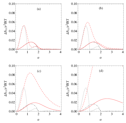
Figure 7: (Color online) Excess noise for Lorentzian pulses of width $\tau_{0}=120\ \mathrm{ps}$ at 1.2 GHz ($f\tau_{0}=0.144$) in the presence of short range interactions in the strong coupling regime, observed at $l/l_{r}$ integer (red dashed curves) and $l/l_{r}$ half-integer (red full curves) as a function of $\alpha$ for various temperatures: (a) $T_{\mathrm{el}}=5\ \mathrm{mK}$, (b) $T_{\mathrm{el}}=10\ \mathrm{mK}$, (c) $T_{\mathrm{el}}=20\ \mathrm{mK}$ and (d) $T_{\mathrm{el}}=40\ \mathrm{mK}$. For comparison, we have replotted the zero temperature results on each panel as dotted and dot-dashed black curves.

IV.2.2 Changing the waveform

However, as can be noticed from figure 7, part of the difficulty arises from the fact that the difference between the minimal and maximal values of excess noise for Lorentzian pulses at zero temperature is not very large and decays with $\alpha$ thus making the effect very fragile against thermal fluctuations. Since this is not the case for rectangular pulsesDubois et al. , a strategy for observing fractionalization might be to consider a rectangular waveform.

We have thus considered rectangular pulses for which, as mentioned before, shorter pulses could then be generated by an AWG. Figure 8 corresponds $\tau_{0}=40~{}\mathrm{ps}$ pulses at the same $1.2$ GHz driving frequency and for the same temperatures as in figure 7. Interactions are assumed to be short range. As expected, the signal is stronger and more robust to the onset of the temperature. Even at 20 mK, the position of the minima for the excess noise exhibit a clear signature of the fractionalization of each $\alpha$ pulse into two $\alpha/2$ pulses. Therefore, although rectangular pulses with integer $\alpha$ are not purely electronic excitations, they indeed appear as good candidates to demonstrate fractionalization at the single pulse level with today’s technology.

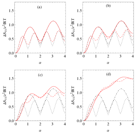
Figure 8: (Color online) Excess noise for rectangular pulses of width $\tau_{0}=40\ \mathrm{ps}$ at 1.2 GHz ($f\tau_{0}=0.048$) in the presence of short range interactions in the strong coupling regime, observed at $l/l_{r}$ integer (red dashed curves) and $l/l_{r}$ half-integer (red full curves) as a function of $\alpha$ for various temperatures: (a) $T_{\mathrm{el}}=5\ \mathrm{mK}$, (b) $T_{\mathrm{el}}=10\ \mathrm{mK}$, (c) $T_{\mathrm{el}}=20\ \mathrm{mK}$ and (d) $T_{\mathrm{el}}=40\ \mathrm{mK}$. For comparison, we have replotted the zero temperature results on each panel as dotted and dot-dashed black curves.

IV.2.3 Long range interactions

We now consider the case of long range interactions modeled using the discrete element model introduced in section IV.1.2. Figure 9 present the case of Lorentzian pulses in the presence of long range interactions with the same parameters as in figure 7. Interaction parameters have been chosen as described in appendix D: we have considered the strong coupling regime $\theta=\pi/2$ and at low frequencies, have estimated the charge velocity as $v_{-}\simeq 7.8\times 10^{6}\ \mathrm{ms}^{-1}$ and the spin velocity as $v_{+}\simeq 4\times 10^{5}\ \mathrm{ms}^{-1}$ which are compatible with known expected values from time of flightKamata et al. (2010); Kumada et al. (2011) and finite frequency admittanceBocquillon et al. (2012) measurements.

At the lowest temperature (graph (a)), the excess noise does not exhibit for a generic length a pronounced minimum at $\alpha=2$ but instead starts decaying with very smooth local minima slightly above each integer value of $\alpha$. Therefore, the signature of fractionalization discussed previously is absent as expected since dispersion strongly alters the shape of the pulses. This induces a much slower decay of the excess noise as a function of $\alpha$ for $l=l_{r}/2$ than in the case of short range interactions. This could be used as a clear signature of the long range character of interactions at very low temperatures. Note that at higher temperature (graphs (d): $T_{\mathrm{el}}=40\ \mathrm{mK}$), only a quantitative comparison between experimental data and theory would enable discriminating between various interaction models.

Considering rectangular waveforms does not radically change the picture: at very low temperature, the difference between short and long range interactions is very clear, this time even more qualitative since for short range interactions, minima of the excess noise in function of $\alpha$ occur for the three lowest temperatures considered (graph (a), (b) and (c) of figure 8) whereas, in the case of long range interactions the excess noise increases rapidly with $\alpha$ (graph (a), (b), (c) and (d) of figure 10). This is qualitatively and quantitatively different from predictions obtained from the short range model.

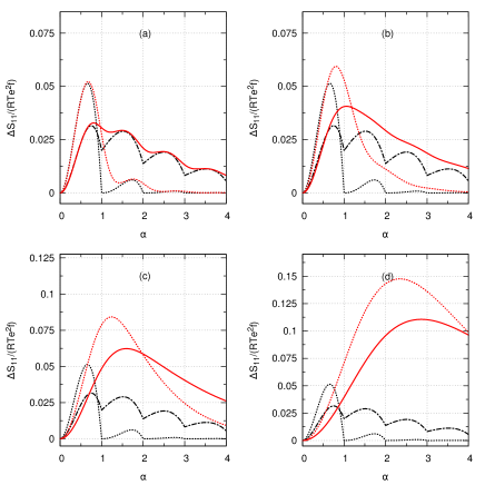
Figure 9: (Color online) Excess noise for Lorentzian pulses of width $\tau_{0}=40\ \mathrm{ps}$ at 1.2 GHz ($f\tau_{0}=0.048$) in the presence of long range interactions in the strong coupling regime, observed at $l/l_{r}$ integer (red dashed curves) and $l/l_{r}$ half-integer (red full curves) as a function of $\alpha$ for various temperatures: (a) $T_{\mathrm{el}}=5\ \mathrm{mK}$, (b) $T_{\mathrm{el}}=10\ \mathrm{mK}$, (c) $T_{\mathrm{el}}=20\ \mathrm{mK}$ and (d) $T_{\mathrm{el}}=40\ \mathrm{mK}$. For comparison, we have replotted the zero temperature results on each panel as dotted and dot-dashed black curves.

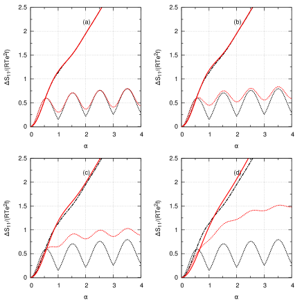
Figure 10: (Color online) Excess noise for rectangular pulses of width $\tau_{0}=120\ \mathrm{ps}$ at 1.2 GHz ($f\tau_{0}=0.144$) in the presence of long range interactions in the strong coupling regime, observed at $l/l_{r}$ integer (red dashed curves) and $l/l_{r}$ half-integer (red full curves) as a function of $\alpha$ for various temperatures: (a) $T_{\mathrm{el}}=5\ \mathrm{mK}$, (b) $T_{\mathrm{el}}=10\ \mathrm{mK}$, (c) $T_{\mathrm{el}}=20\ \mathrm{mK}$ and (d) $T_{\mathrm{el}}=40\ \mathrm{mK}$. For comparison, we have replotted the zero temperature results on each panel as dotted and dot-dashed black curves.

V Conclusion

In a system of two copropagating edge channels, interactions lead to charge fractionalization. We propose to detect this phenomenon at the single excitation level by monitoring the electron/hole pair production of voltage pulses as a function of their charge. More precisely, electron/hole pair production presents a minima each time an integer charge pulse is fractionalized into two pulses of integer charges.

To discuss the observability of this phenomenon in realistic experiments, we have studied the excess noise coming out of and HBT interferometer fed by a periodic train or Lorentzian or rectangular pulses. Although experimentally challenging, our study suggests that Lorentzian pulses of short enough durations could also be used to probe in detail the physics of fractionalization: beyond the characterization of electron/hole pair production, current noise measurement in the Hanbury Brown and Twiss setup can be used to perform a lest a spectroscopyDubois et al. and, ultimately, a full tomographyGrenier et al. (2011b) of fractional charge collective excitations. We have also shown that fractionalization of rectangular pulses could be observed with state of the art microwave waveform generators and that, for Lorentzian pulses, it might be within reach in the near future using optical techniques to generate periodic train of a few picosecond wide pulses at high repetition rates.

We have also shown that fractionalization is very sensitive to the range of interaction which governs the dispersion of edge magnetoplasmon eigenmodes: long range interactions might prevent observing fractionalization. Nevertheless, the dependence of the excess noise signal in the charge of the pulses and in the propagation length gives information on the interaction range. Since our experimental setup could also be used to perform high frequency admittance measurements in the $\nu=2$ edge channel systemBocquillon et al. , it opens the way to “on chip” consistency checks of the edge magnetoplasmon scattering approach never realized before.

These results argue for the development of experiments aimed at studying interaction induced electron/hole pair generation in the $\nu=2$ quantum Hall edge channel system. In particular, performing such experiments on samples with side-gated copropagating edge channels as in recent experiments by F. Pierre et alLe Sueur et al. (2010) as well as on samples without gating might be a good way to access various interaction ranges.

An important issue of great interest is the influence of edge smoothness on the electronic transport properties of the edge channels. Several authorsAleiner and Glazman (1994); Aleiner et al. (1995); Han and Thouless (1997); Johnson and Vignale (2003) have predicted the appearance of several branches of neutral excitations at the edge of a 2DEG in the integer quantum Hall regime as well as dissipation for these all the gapless edge modes. But their existence has not been directly demonstrated so far. Studying electron/hole pair production along propagation of voltage pulses and performing high frequency admittance measurements could help clarifying this issue and understand the dynamics of the all gapless modes living at the edge of the 2DEG in the integer quantum Hall regime.

Appendix A Photo assisted transition amplitudes

Here, we compute the photo-assisted transition amplitudes in presence of the periodic AC voltage $V_{\mathrm{ac}}(t)$ for the Lorentzian and square pulses.

A.1 Rectangular pulses

Let us consider square pulses of width $\tau_{0}\leq T$, defined for $|t|\leq T/2$ by $V(t)=-\alpha h/e\tau_{0}$ for $|t|\leq\tau_{0}/2$, $V(t)=0$ for $|t|>\tau_{0}/2$. For a $T$-periodic train of such pulses, the Floquet amplitudes $C_{l}(\alpha,f\tau_{0})$ are given by:

$$C_{l}(\alpha,f\tau_{0}) = (-1)^{l}\frac{\sin{(\pi(l+\alpha)(1-f\tau_{0}))}}{\pi(l+\alpha)}$$ (24)

$$+ f\tau_{0}\frac{\sin{(\pi\alpha-\pi(l+\alpha)f\tau_{0})}}{\pi\alpha-\pi(l+\alpha)f\tau_{0}}\,.$$

In the limit $f\tau_{0}\rightarrow 1$, these amplitudes vanish reflecting the fact that the ac part of the voltage drive vanishes at $f\tau_{0}=1$. These amplitudes are also obtained as $C_{l}=C(2\pi f(l+\alpha))$ where

$$C(\omega)=\frac{2}{\omega T}\left(\pi\alpha\,\mathrm{sinc}{\left(\frac{\omega\tau_{0}}{2}-\pi\alpha\right)}+\sin{\left(\frac{\omega T}{2}-\pi\alpha\right)}\right)$$ (25)

where $\mathrm{sinc}(x)=\sin{(x)}/x$. In the limit $f\tau_{0}\ll 1$, the main contribution to the partition noise arises from the squared modulus of the first term in the r.h.s of (25). At zero temperature, the discrete sum (17) is a regularized expression for the integral expression for the noise

$$\Delta S_{1,1}^{(\mathrm{out})}\simeq\mathcal{RT}(\alpha e)^{2}f\int\mathrm{sinc}^{2}{\left(\frac{\omega\tau_{0}-2\pi\alpha}{2}\right)}\,\frac{d\omega}{|\omega|}$$ (26)

originally considered by Lee and LevitovLee and Levitov . As expected, this expression exhibits an IR logarithmic divergence when $\alpha$ is not an integer which is a signature of the orthogonality catastrophe associated with the fractional charge pulsesLee and Levitov . For a periodic train of pulsesDubois et al. , this divergence is regularized by the period but manifests itself as a logarithmic divergence of the outcoming excess noise $\Delta S_{1,1}^{(\mathrm{out})}$ in the limit $f\tau_{0}\rightarrow 0$. When $\alpha$ is integer, the logarithmic divergence at $\omega=0$ is replaced by a peak.

Note that the integrand in (26) always has a peak for $\omega\tau_{0}=2\pi\alpha$ and an $|\omega|^{-3}$ behavior at large $|\omega|$.

A.2 Lorentzian pulses

The amplitude $C_{l}(\alpha,q)$ to absorb $n$ photons can be computed as a contour integral ($q=e^{-2\pi f\tau_{0}}$):

$$C_{l}(\alpha,q)=\oint_{|z|=1}z^{l+\alpha-1}\left(\frac{1-qz}{z-q}\right)^{\alpha}\,\frac{dz}{2\pi i}\,.$$ (27)

When $\alpha$ is a positive integer, the integrand has a pole of order $\alpha$ for $z=q$ and when $l+\alpha\leq 0$ another pole of order $1-(l+\alpha)$ at $z=0$. Since for $l<-\alpha$ the integral can be computed by closing the contour at infinity, this immediately shows that $C_{l}(\alpha,q)=0$ for $l<-\alpha$. In the general situation where $\alpha>0$ is not an integer, the integrand presents a branch cut singularity connecting $z=0$ to $z=q$ along the real axis and another one connecting $z=1/q$ to $z=\infty$.

For $0<\alpha<1$, deforming the unit circle around the appropriate branch cut leads to expressions for the photo-assisted amplitudes in terms of hypergeometric functions. Expanding these functions in series of $q^{2}$ and using the complement formula for the $\Gamma$ function leads to new series expansions of $C_{l}(\alpha,q)$ in $q$ in which the cancellation of $C_{l}$ for $l+\alpha<0$ and $\alpha$ integer is manifest. For $l+\alpha\geq 0$

$$C_{l}(\alpha,q)=\alpha\sum_{k=0}^{+\infty}\frac{\Gamma(k+l+\alpha)\,q^{l+k}}{\Gamma(l+k+1)}\,\frac{(-q)^{k}}{k!\,\Gamma(1+\alpha-k)}$$ (28)

whereas for $l+\alpha\leq 0$,

$$C_{l}(\alpha,q)=\alpha\sum_{k=0}^{+\infty}\frac{\Gamma(l+k+\alpha)\,(-q)^{l+k}}{\Gamma(l+k+1)}\,\frac{q^{k}}{k!\,\Gamma(1+\alpha-k)}\,.$$ (29)

When $\alpha$ is a positive integer, due to the $\Gamma(1+\alpha-k)$ at the denominator, the sum over $k$ is truncated to $k\leq\alpha$. For the same reason, terms with $k\geq-1-l$ vanish when $l\leq-1$. Consequently $C_{l}(\alpha,q)$ is a polynomial in $q$ for $l+\alpha\geq 0$ and $C_{l}(\alpha,q)=0$ for $l+\alpha\leq 0$. Note that for non integer $\alpha>0$, the vanishing of terms with $k\geq\alpha+1$ does not happen: both expressions are full series in $q$ and therefore do not vanish. In the case of a high compacity source $f\tau_{0}\gg 1$ or equivalently $q\rightarrow 0$ and consequently, all $C_{l}(\alpha,q)$ vanish for $l\neq 0$ and $C_{0}(\alpha,q)\rightarrow 1$ as expected since in this limit the AC voltage vanishes.

Appendix B Electron and hole excitations

The operators counting the number of electrons and holes excitations with respect to the Fermi level are defined by:

$$N_{e} = \int_{0}^{+\infty}c^{\dagger}(\omega)\,c(\omega)\,d\omega$$ (30)

$$N_{h} = \int_{-\infty}^{0}c(\omega)\,c^{\dagger}(\omega)\,d\omega\,.$$ (31)

Their averages can then be obtained in terms of the single electron and single hole coherences:

$$\langle N_{e}\rangle = \frac{iv_{F}}{2\pi}\int\frac{\mathcal{G}^{(e)}(t,t^{\prime})}{t-t^{\prime}+i0^{+}}\,dt\,dt^{\prime}$$ (32)

$$\langle N_{h}\rangle = -\frac{iv_{F}}{2\pi}\int\frac{\mathcal{G}^{(h)}(t^{\prime},t)}{t-t^{\prime}-i0^{+}}\,dt\,dt^{\prime}\,.$$ (33)

In an Hanbury Brown and Twiss experiment, the current noise in the outcoming arms contains a contribution of the current noises within each of the two incoming channels denoted here by $1$ and $2$ and a contribution $\mathcal{Q}$ due to two particle interferencesGrenier et al. (2011b):

$$S_{1,1}^{(\mathrm{out})}=\mathcal{R}^{2}S_{1,1}^{(\mathrm{in})}+\mathcal{T}^{2}S_{2,2}^{(\mathrm{in})}+\mathcal{RT}\mathcal{Q}$$ (34)

where $\mathcal{R}$ and $\mathcal{T}$ respectively denote the energy independent reflexion and transmission probabilities of the QPC used to partition the incident electron beams. The Hanbury Brown and Twiss contribution $\mathcal{Q}$ can be expressed in terms of the overlap of single electron coherences within the two incoming channelsGrenier et al. (2011b):

$$\mathcal{Q}=(ev_{F})^{2}\int(\mathcal{G}^{(e)}_{1}\mathcal{G}^{(h)}_{2}+\mathcal{G}^{(h)}_{1}\mathcal{G}^{(e)}_{2})(t,t^{\prime})\,dt\,dt^{\prime}\,.$$ (35)

Using the electron and hole coherences of the Fermi sea at zero temperature for $\mathcal{G}_{2}^{(e/h)}(t,t^{\prime})$ shows that $\mathcal{Q}=e^{2}\left(\langle N_{e}\rangle+\langle N_{h}\rangle\right)$, thus showing that low frequency noise measurements lead to the measurement of the total number of excitations at zero temperature.

In the case of a voltage pulse, the single electron coherence is given by (3) and in a similar way:

$$\mathcal{G}_{1}^{(h)}(t^{\prime},t)=\frac{i}{2\pi v_{F}}\,\frac{e^{i(\phi_{V}(t)-\phi_{V}(t^{\prime}))}}{t-t^{\prime}-i0^{+}}\,.$$ (36)

where $\phi_{V}(t)=\frac{e}{\hbar}\int_{0}^{t}V(\tau)\,d\tau$. Substituting (3) and (36) into (35) leads to the following expression for the total number of excitations:

$$\langle N_{e}+N_{h}\rangle=\int\kappa(t-t^{\prime})e^{i(\phi_{V}(t)-\phi_{V}(t^{\prime}))}\,dt\,dt^{\prime}$$ (37)

where the kernel $\kappa(t-t^{\prime})$ is given by

$$\kappa(\tau)=\frac{1}{(2\pi)^{2}}\left(\frac{1}{(\tau+i0^{+})^{2}}+\frac{1}{(\tau-i0^{+})^{2}}\right)\,.$$ (38)

Minimizing this quantity is precisely the problem solved by Levitov, Lee and Lesovik in their 1996 paperLevitov et al. (1996).

In the case of a $T$-periodic source, this discussion must be adapted by considering a time average over a single period. Since experiments are performed at non zero temperature, the HBT contribution to the noise signals is altered by the anti bunching of electron and holes excitations emitted by the source and the thermal electron and hole excitations emitted from the second incoming channel. Here we are interested by the excess contribution due to the AC part $V_{\mathrm{ac}}(t)$ of the drive voltage. Denoting the chemical potential of the second incoming channel by $\mu_{2}$ and its electronic temperature by $T_{\mathrm{el}}$, the excess HBT contribution is given in terms of the excess single electron coherence generated by the AC drive:

$$\Delta\mathcal{Q}=e^{2}\int_{-\infty}^{+\infty}\tanh{\left(\frac{\hbar\omega-\mu_{2}}{2k_{B}T_{\mathrm{el}}}\right)}\,\frac{v_{F}}{2\pi}\Delta\mathcal{G}_{1,0}^{(e)}(\omega)\,d\omega\,.$$ (39)

When $\mu_{2}=\mu_{1}$ (here conveniently set to zero), equation (16) can then be expressed in terms of the excess spectral density of electron and hole excitations $\Delta\bar{N}_{e}(\omega)$ and $\Delta\bar{N}_{h}(\omega)$ emitted per period by the source at energy $\hbar\omega>0$:

$$\frac{\Delta\mathcal{Q}}{e^{2}f}=\int_{0}^{+\infty}\tanh{\left(\frac{\hbar\omega}{2k_{B}T_{\mathrm{el}}}\right)}\,\Delta(\bar{N}_{e}+\bar{N}_{h})(\omega)\,d\omega\,.$$ (40)

since these excess electron and hole per period spectral densities are related to the single electron coherence byGrenier et al. (2011b):

$$\Delta\bar{N}_{e}(\omega) = \frac{v_{F}}{2\pi f}\,\Delta\mathcal{G}_{1,0}^{(e)}(\omega)$$ (41)

$$\Delta\bar{N}_{h}(\omega) = -\frac{v_{F}}{2\pi f}\,\Delta\mathcal{G}_{1,0}^{(e)}(-\omega)\,.$$ (42)

Appendix C Finite temperatures and interactions

At non zero temperature $T_{\mathrm{el}}$, an Ohmic contact emits an equilibrium state which can equivalently be described both in terms of electrons and in terms of edge magnetoplasmon excitations. In the latter description, this state is the thermal state at temperature $T_{\mathrm{el}}$ of the bosonic excitations above the Fermi vacuum $|F_{\mu+\alpha hf}\rangle$ which is a vacuum state for the edge magnetoplasmon modes.

This thermal state can also be understood as a Gaussian statistical mixture of edge magnetoplasmon coherent states $|[\delta\Lambda(\omega)]\rangle$. This Gaussian distribution is centered around the vacuum $\Lambda(\omega)=0$ for all $\omega>0$. Its fluctuations $\overline{\delta\Lambda(\omega)\delta\Lambda^{*}(\omega^{\prime})}$ are then equal to the thermal average of the edge magnetoplasmon number $\langle b^{\dagger}(\omega)b(\omega^{\prime})\rangle$ in the thermal equilibrium state at temperature $T_{\mathrm{el}}$:

$$\overline{\delta\Lambda(\omega)\delta\Lambda^{*}(\omega^{\prime})}_{T_{\mathrm{el}}}=\delta(\omega-\omega^{\prime})\bar{n}(\omega,T_{\mathrm{el}})$$ (43)

where $\bar{n}(\omega,T_{\mathrm{el}})$ denotes here the Bose-Einstein occupation number $1/(e^{\hbar\omega/k_{B}T_{\mathrm{el}}}-1)$.

As in quantum optics, applying a time dependent drive voltage to the Ohmic contact corresponds to applying a displacement operator to this thermal state. The resulting displaced thermal state can then be described as a Gaussian statistical mixtures of edge magnetoplasmon coherent states around $\Lambda_{V}$ given by eq. (20) and with fluctuations given by (43).

To understand the action of the interaction region onto two such displaced thermal states, let us first consider two incoming coherent states from the statistical ensembles defining the two displaced thermal states. They are characterized by their infinite dimensional complex parameters $\Lambda_{a}^{(\mathrm{in})}$ with $a=1$ or $2$. The outcoming states is then a tensor product of two coherent states characterized by

$$\left(\begin{array}[]{c}\Lambda_{1}^{(\mathrm{out})}\\ \Lambda_{2}^{(\mathrm{out})}\end{array}\right)=S\ldotp\left(\begin{array}[]{c}\Lambda_{1}^{(\mathrm{in})}\\ \Lambda_{2}^{(\mathrm{in})}\end{array}\right)$$ (44)

Decomposing the incoming coherent state parameters into their averages and their Gaussian fluctuations $\Lambda_{a}^{(\mathrm{in})}=\Lambda_{a}+\delta\Lambda_{a}$ ($a=1,2$) shows that, for each outcoming chanel, we have a Gaussian statistical mixture of coherent states. The corresponding Gaussian distribution of the complex parameters is centered around the classical outcoming parameters obtained by applying the edge magnetoplasmon scattering matrix onto the vector of incoming parameters $(\Lambda_{a})_{a=1,2}$: this is nothing but the scattering for wave amplitudes by a frequency dependent beamsplitter in optics. The outcoming fluctuations in each channel are Gaussian but nevertheless do not correspond to any thermal equilibrium as noticed by Kovrizhin and ChalkerKovrizhin and Chalker (2011). The outcoming fluctuations are given by:

$$\langle b_{a}^{\dagger}(\omega)b_{a^{\prime}}(\omega^{\prime})\rangle_{c}^{(\mathrm{out})} = \delta_{a,a^{\prime}}\delta(\omega-\omega^{\prime})\,\bar{n}_{\mathrm{out}}(\omega)$$ (45)

$$\bar{n}_{\mathrm{out}}(\omega) = \sum_{b}|S_{a,b}(\omega)|^{2}\,\bar{n}(\omega,T_{b})$$ (46)

where the $c$ subscript stands for ”connected” and $T_{b}$ denotes the temperature of the incoming channel $b$. When all the incoming channels have the same temperature $T_{\mathrm{el}}$, a thermal distribution is recovered due to the unitarity of the edge magnetoplasmon scattering matrix: $\sum_{b}|S_{a,b}(\omega)|^{2}=1$.

Appendix D Magnetoplasmon scattering for long range interactions

Let us denote by $Q_{j}(t)$ the charge stored within the interacting region of edge channel $j$. These charges are determined from the electrostatic potential $U_{j}(t)$ seen by electrons propagating in edge channel $j$ within the interacting region through a capacitance matrix:

$$\left(\begin{array}[]{c}Q_{1}(t)\\ Q_{2}(t)\end{array}\right)=\left(\begin{array}[]{cc}C_{1}&-C\\ -C&C_{2}\end{array}\right)\ldotp\left(\begin{array}[]{c}U_{1}(t)\\ U_{2}(t)\end{array}\right)\,.$$ (47)

Assuming both edge channels have the same Fermi velocity $v_{F}$, the dynamics of channel $j$ is determined by the equation of motion

$$(\partial_{t}+v_{F}\partial_{x})\phi_{j}(x,t)=\frac{e\sqrt{\pi}}{h}\,f(x)U_{j}(t)$$ (48)

where $f(x)=1$ for $0\leq x\leq l$ and zero otherwise. The strategy is then to go to the frequency domain and rewrite eqs. (47) and (48) in terms of the incoming and outcoming bosonic field amplitudes and to eliminate the potentials $U_{j}(\omega)$. More precisely, in order to rewrite (47) in terms of the incoming and out coming bosonic fields, one has to use the relation between the electronic density within each edge channel and the corresponding bosonic field: $:\psi^{\dagger}_{j}\psi_{j}(x):=(\partial_{x}\phi_{j})(x)/\sqrt{\pi}$. Because (47) involves the capacitance matrix, eliminating the potentials $U_{j}(\omega)$ is most conveniently performed after diagonalizing $\mathcal{C}$ with a rotation $R_{\theta}=\cos{(\theta/2)}\mathbf{1}-i\sin{(\theta/2)}\sigma^{y}$. This finally leads to the scattering matrix:

$$S(\omega,l)=R_{\theta}^{-1}\,\left(\begin{array}[]{cc}\mathcal{T}_{+}(\omega,l)&0\\ 0&\mathcal{T}_{-}(\omega,l)\end{array}\right)R_{\theta}$$ (49)

where the angle $\theta$ is given by ($\Delta C=C_{1}-C_{2}$):

$$\exp{(i\theta)}=\frac{\Delta C/2+i\,C}{\sqrt{C^{2}+\frac{\Delta C^{2}}{4}}}\,$$ (50)

and the phases $\mathcal{T}_{\pm}(\omega,l)$ have a non linear (dispersive) $\omega$ dependence given by:

$$\mathcal{T}_{\pm}(\omega,l)=e^{i\omega l/v_{F}}\,\frac{i\omega R_{K}C_{\pm}+1-e^{-i\omega l/v_{F}}}{i\omega R_{K}C_{\pm}-1+e^{i\omega l/v_{F}}}\,$$ (51)

where the eigenvalues of the capacitance matrix are

$$C_{\pm}=\frac{C_{1}+C_{2}}{2}\pm\sqrt{C^{2}+\frac{\Delta C^{2}}{4}}\,.$$ (52)

The exponential $e^{i\omega l/v_{F}}$ in the r.h.s. of (51) represents the effect of free propagation and the other part contains the effect of the capacitances. Note that the free propagation limit is obtained for infinite capacitances $C_{\pm}$. At low frequencies, the plasmon eigenmodes become dispersionless: $\mathcal{T}_{\pm}(\omega,l)\simeq e^{i\omega l/v_{\pm}}$ where the velocities $v_{\pm}$ are given by

$$v_{\pm}=v_{F}+\frac{l}{R_{K}C_{\pm}}\,.$$ (53)

Capacitances being proportional to $l$, the velocities $v_{\pm}$ are independent from $l$: $v_{\pm}=v_{F}+(R_{K}\partial_{l}C_{\pm})^{-1}$. Therefore, in the infrared regime, the plasmon scattering matrix is of the form (21). An explicit check shows that the admittance matrix satisfies charge conservation and gauge invariance if and only if the capacitance matrix satisfies the same condition. In such a case, each edge channel is totally screened by the other one within the interaction region.

It is interesting to evaluate the order of magnitudes of the various capacitances. We consider each edge channel as a quasi 1D conductor of length $l$ very large compared to its transverse dimensions $w$ as well as to the distance $d$ between the two conductors. Then, the capacitances are of the form

$$C_{i,j}=\frac{\varepsilon_{r}\varepsilon_{0}}{l}\,F_{i,j}(w,d)$$ (54)

where $\varepsilon_{r}$ denotes the relative permittivity of the material and $F_{i,j}(w,d)$ is a dimensionless function of $w$ and $d$ that depends on the geometry. The dimensionless ratios of the $RC$ times to the time of flight $l/v_{F}$ are then given by:

$$\frac{v_{F}R_{K}C_{i,j}}{l}=\frac{\varepsilon_{r}}{4\pi\alpha_{\mathrm{qed}}}\,\frac{v_{F}}{c}\,F_{i,j}(w,d)$$ (55)

where $\alpha_{\mathrm{qed}}$ denotes the fine structure constant. Using $v_{F}\simeq 3\times 10^{5}\ \mathrm{ms}^{-1}$ and $\varepsilon_{r}\simeq 10$ for $\mathrm{AsGa}$, one gets a numerical prefactor $v_{F}\varepsilon_{r}/4\pi c\alpha_{\mathrm{qed}}\simeq 0.4$.

Let us now consider the case where $C_{1}=C_{2}$ so that $\theta=\pi/2$. The model then only depends on the diagonal capacitances $C_{d}$ and the mutual capacitance between the two channels $C$. If we furthermore assume that perfect screening is closed to be achieved, $C_{d}$ and $C$ are close together. Introducing $C_{\pm}=C_{d}\pm C$, we see that $C_{-}\ll C_{+}$ and therefore the two velocities (53) satisfy $v_{+}\ll v_{-}$. Note that here $v_{-}$ is the velocity of the symmetric (charge) mode whereas $v_{+}$ is the velocity of the antisymmetric (dipolar) mode which, as in the case of short range interactions, is the slowest one. For example using (55) and $F_{11}=F_{22}=1$, we find $v_{F}R_{K}C_{+}/l\simeq 0.8$ leading to $v_{+}/v_{F}\simeq 1.25$. Consequently, the slowest velocity is of the order of $v_{+}\simeq 4\times 10^{5}~{}\mathrm{ms}^{-1}$. Assuming $C_{d}-C\simeq 0.05\times(C_{d}+C)$, we have $v_{-}/v_{F}\simeq 26$ thus leading to $v_{-}\simeq 7.8\times 10^{6}~{}\mathrm{ms}^{-1}$, a value of the same order of magnitude than the experimentally measured edge magnetoplasmon velocities in ungated samples at filling fraction $\nu=2$Kumada et al. (2011).

The numerical computations in section IV.2 are performed using the following expression for the scattering phase in terms of the dimensionless parameter $x=\omega l/v_{F}$:

$$\mathcal{T}_{\pm}(\omega,l)=\frac{e^{ix}-1+i\alpha_{\pm}x\,e^{ix}}{e^{ix}-1+i\alpha_{\pm}x}\,$$ (56)

where $\alpha_{\pm}=R_{K}C_{\pm}v_{F}/l=v_{F}R_{K}\partial_{l}C_{\pm}$. Note that this expression is clearly not periodic in $x\rightarrow x+1$ whereas it is equal to one whenever $x$ is an integer. Under the hypothesis $C_{1}=C_{2}$ and very good screening, $\alpha_{-}\ll\alpha_{+}$. Using the above numerical estimations: $\alpha_{+}\simeq 0.8$ and $\alpha_{-}\simeq 0.04$.

References

- Ji et al. (2003) Y. Ji, Y. Chung, D. Sprinzak, M. Heiblum, D. Mahalu, and H. Shtrikman, Nature 422, 415 (2003).
- Neder et al. (2007) I. Neder, F. Marquardt, M. Heiblum, D. Mahalu, and V. Umansky, Nature Physics 3, 534 (2007).
- Roulleau et al. (2007) P. Roulleau, F. Portier, D. C. Glattli, P. Roche, A. Cavanna, G. Faini, U. Gennser, and D. Mailly, Phys. Rev. B 76, 161309 (2007).
- Roulleau et al. (2008a) P. Roulleau, F. Portier, P. Roche, A. Cavanna, G. Faini, U. Gennser, and D. Mailly, Phys. Rev. Lett. 101, 186803 (2008a).
- Roulleau et al. (2008b) P. Roulleau, F. Portier, D. C. Glattli, P. Roche, A. Cavanna, G. Faini, U. Gennser, and D. Mailly, Phys. Rev. Lett. 100, 126802 (2008b).
- Litvin et al. (2007) L.V. Litvin, H.-P. Tranitz, W. Wegscheider, and C. Strunk, Phys. Rev. B 75, 033315 (2007).
- Chalker et al. (2007) J.T. Chalker, Y. Gefen, and M.Y. Veillette, Phys. Rev. B 76, 085320 (2007).
- Levkivskyi and Sukhorukov (2008) I.P. Levkivskyi and E.V. Sukhorukov, Phys. Rev. B 78, 045322 (2008).
- Kovrizhin and Chalker (2009) D. L. Kovrizhin and J. T. Chalker, Phys. Rev. B 80, 161306 (2009).
- Neuenhahn and Marquardt (2008) C. Neuenhahn and F. Marquardt, New Journal of Physics 10, 115018 (2008).
- Neder and Marquardt (2007) I. Neder and F. Marquardt, New Journal of Physics 9, 112 (2007).
- Fève et al. (2007) G. Fève, A. Mahé, J. Berroir, T. Kontos, B. Plaçais, D. C. Glattli, A. Cavanna, B. Etienne, and Y. Jin, Science 316, 1169 (2007).
- Mahé et al. (2010) A. Mahé, F.D. Parmentier, E. Bocquillon, J.M. Berroir, D.C. Glattli, T. Kontos, B. Plaçais, G. Fève, A. Cavanna, and Y. Jin, Phys. Rev. B 82, 201309 (2010).
- Henny et al. (1999) M. Henny, S. Oberholzer, C. Strunk, T. Heinzel, K. Ensslin, M. Holland, and C. Schönenberger, Science 284, 296 (1999).
- Oliver et al. (1999) W. Oliver, J. Kim, R. Liu, and Y. Yamamoto, Science 284, 299 (1999).
- Bocquillon et al. (2012) E. Bocquillon, F.D. Parmentier, C. Grenier, J.M. Berroir, P. Degiovanni, D.C. Glattli, B. Plaçais, A. Cavanna, Y. Jin, and G. Fève, Phys. Rev. Lett. 108, 196803 (2012).
- Grenier et al. (2011a) C. Grenier, R. Hervé, G. Fève, and P. Degiovanni, Mod. Phys. Lett. B 25, 1053 (2011).
- Leicht et al. (2011) C. Leicht, P. Mirovsky, B. Kaestner, F. Hols, V. Kashcheyevs, E. Kurganova, U. Zeitler, T. Weimann, K. Pierz, and H. Schumacher, Semicond. Sci. Technol. 26, 055010 (2011).
- Hohls et al. (2012) F. Hohls, A.C. Welker, Ch. Leicht, L. Fricke, B. Kaestner, P. Mirovsky, A. Muller, K. Pierz, U. Siegner, and H.W. Schumacher, Phys. Rev. Lett. 109, 056802 (2012).
- Talyanskii et al. (1997) V. I. Talyanskii, J. M. Shilton, M. Pepper, C. G. Smith, C. J. B. Ford, E. H. Linfield, D. A. Ritchie, and G. A. C. Jones, Phys. Rev. B 56, 15180 (1997).
- Blumenthal et al. (2007) M. Blumenthal, B. Kaestner, L. Li, S. Giblin, T. Janssen, M. Pepper, D. Anderson, G. Jones, and D. Ritchie, Nature Physics 3, 343 (2007).
- Ahlers et al. (2006) F.-J. Ahlers, O. Kieler, B. Sagol, K. Pierz, and U. Siegner, Journal of Applied Physics 100, 093702 (2006).
- Kaestner et al. (2008) B. Kaestner, V. Kashcheyevs, S. Amakawa, M. D. Blumenthal, L. Li, T. J. B. M. Janssen, G. Hein, K. Pierz, T. Weimann, U. Siegner, and H. W. Schumacher, Phys. Rev. B 77, 153301 (2008).
- Fujiwara et al. (2008) A. Fujiwara, F. Nishiguchi, and Y. Ono, Applied Physics Letters 92, 042102 (2008).
- Landau (1959) L. Landau, Sov. Phys. JETP 35, 70 (1959).
- Pines and Nozières (1966) D. Pines and P. Nozières, The theory of quantum liquids (Perseus Book, 1966).
- Degiovanni et al. (2009) P. Degiovanni, C. Grenier, and G. Fève, Phys. Rev. B 80, 241307(R) (2009).
- Levitov et al. (1996) L. Levitov, H. Lee, and G. Lesovik, J. Math. Phys. 37, 4845 (1996).
- Ivanov et al. (1997) D. A. Ivanov, H. W. Lee, and L. S. Levitov, Phys. Rev. B 56, 6839 (1997).
- Keeling et al. (2006) J. Keeling, I. Klich, and L.S. Levitov, Phys. Rev. Lett. 97, 116403 (2006).
- Hassler et al. (2008) F. Hassler, M.V. Suslov, G.M. Graf, M.V. Lebedev, G.B. Lesovik, and G. Blatter, Phys. Rev. B 78, 165330 (2008).
- Su et al. (1979) W.P. Su, J.R. Schrieffer, and A.J. Heeger, Phys. Rev. Lett. 42, 1698 (1979).
- Altimiras et al. (2010a) C. Altimiras, H. le Sueur, U. Gennser, A. Cavanna, D. Mailly, and F. Pierre, Nature Physics 6, 34 (2010a).
- Le Sueur et al. (2010) H. le Sueur, C. Altimiras, U. Gennser, A. Cavanna, D. Mailly, and F. Pierre, Phys. Rev. Lett. 105, 056803 (2010).
- Altimiras et al. (2010b) C. Altimiras, H. le Sueur, U. Gennser, A. Cavanna, D. Mailly, and F. Pierre, Phys. Rev. Lett. 105, 226804 (2010b).
- Safi et al. (1995) I. Safi and H. Schulz, in Quantum Transport in Semiconductor Submicron Structures, 159 (Kluwer Academic Press, Dordrecht, 1995).
- Pham et al. (2000) K.V. Pham, M. Gabay, and P. Lederer, Phys. Rev. B 61, 16397 (2000).
- Trauzettel et al. (2004) B. Trauzettel, I. Safi, F. Dolcini, and H. Grabert, Phys. Rev. Lett. 92, 226405 (2004).
- Steinberg et al. (2008) H. Steinberg, G. Barak, A. Yacoby, L.N. Pfeiffer, K.W. West, B.I. Halperin, and K. Le Hur, Nature Physics 4, 116 (2008).
- Neder (2012) I. Neder, Phys. Rev. Lett. 108, 186404 (2012).
- Grenier et al. (2011b) C. Grenier, R. Hervé, E. Bocquillon, F. Parmentier, B. Plaçais, J. Berroir, G. Fève, and P. Degiovanni, New Journal of Physics 13, 093007 (2011b).
- (42) J. Dubois, T. Jullien, C. Grenier, P. Degiovanni, P. Roulleau, and D. C. Glattli, preprint ArXiv:1212.3921
- Degiovanni et al. (2010) P. Degiovanni, C. Grenier, G. Fève, C. Altimiras, H. le Sueur, and F. Pierre, Phys. Rev. B 81, 121302(R) (2010).
- Levkivskyi and Sukhorukov (2012) I.P. Levkivskyi and E.V. Sukhorukov, Phys. Rev. B 85, 075309 (2012).
- Neuenhahn and Marquardt (2009) C. Neuenhahn and F. Marquardt, Phys. Rev. Lett. 102, 046806 (2009).
- (46) E. Bocquillon, V. Freulon, J. Berroir, P. Degiovanni, B. Plaçais, A. Cavanna, Y. Jin, and G. Fève, submitted.
- Glauber (1963) R. Glauber, Phys. Rev. 130, 2529 (1963).
- Haack et al. (2011) G. Haack, M. Moskalets, J. Splettstoesser, and M. Büttiker, Phys. Rev. B 84, 081303 (2011).
- Haack et al. (2012) G. Haack, M. Moskalets, and M. Büttiker (2012), preprint ArXiv:1212.0088.
- Lvovsky and Raymer (2009) A. I. Lvovsky and M. G. Raymer, Rev. Mod. Phys. 81, 299 (2009).
- Moskalets and Büttiker (2011) M. Moskalets and M. Büttiker, Phys. Rev. B 83, 035316 (2011).
- Moskalets and Büttiker (2002) M. Moskalets and M. Büttiker, Phys. Rev. B 66, 205320 (2002).
- Moskalets (2011) M. Moskalets, Scattering matrix approach to non-stationary quantum transport (Imperial College Press, London, 2011).
- Jonckheere et al. (2012) T. Jonckheere, T. Stoll, J. Rech, and T. Martin, Phys. Rev. B 85, 045321 (2012).
- Tien and Gordon (1963) P. K. Tien and J. P. Gordon, Phys. Rev. 129, 647 (1963).
- Kato et al. (2005) M. Kato, K. Fujiura, and T. Kurihara, Appl. Opt. Lett. 44 (2005).
- Vanević et al. (2008) M. Vanević, Y. V. Nazarov, and W. Belzig, Phys. Rev. B 78, 245308 (2008).
- Gabelli and Reulet (2012) J. Gabelli and B. Reulet (2012), preprint ArXiv:1205.3638.
- Lesovik and Levitov (1994) G.B. Lesovik and L.S. Levitov, Phys. Rev. Lett. 72, 538 (1994).
- Pedersen and Büttiker (1998) M. H. Pedersen and M. Büttiker, Phys. Rev. B 58, 12993 (1998).
- Rychkov et al. (2005) V. S. Rychkov, M. L. Polianski, and M. Büttiker, Phys. Rev. B 72, 155326 (2005).
- Schoelkopf et al. (1998) R. J. Schoelkopf, A. A. Kozhevnikov, D. E. Prober, and M. J. Rooks, Phys. Rev. Lett. 80, 2437 (1998).
- Reydellet et al. (2003) L.-H. Reydellet, P. Roche, D. C. Glattli, B. Etienne, and Y. Jin, Phys. Rev. Lett. 90, 176803 (2003).
- (64) H. Lee and L. Levitov, preprint ArXiv:cond-mat:9312013.
- Safi (1999) I. Safi, Eur. Phys. J. D 12, 451 (1999).
- Safi and Schulz (1995) I. Safi and H. Schulz, in Quantum Transport in Semiconductor Submicron Structures, edited by B. Kramer (Kluwer Academic Press, Dordrecht, 1995), p. 159.
- Lebedev and Blatter (2011) A.V. Lebedev and G. Blatter, Phys. Rev. Lett. 107, 076803 (2011).
- Büttiker et al. (1993) M. Büttiker, A. Prêtre, and H. Thomas, Phys. Rev. Lett. 70, 4114 (1993).
- Prêtre et al. (1996) A. Prêtre, H. Thomas, and M. Büttiker, Phys. Rev. B 54, 8130 (1996).
- Christen and Büttiker (1996) T. Christen and M. Büttiker, Phys. Rev. B 53, 2064 (1996).
- Han and Thouless (1997) J.H. Han and D.J. Thouless, Phys. Rev. B 55, R1926 (1997).
- Parmentier et al. (2011) F. Parmentier, A. Mahé, A. Denis, J.-M. Berroir, D. C. Glattli, B. Plaçais, and G. Fève, Rev. Sci. Instrum. 82, 013904 (2011).
- Kamata et al. (2010) H. Kamata, T. Ota, K. Muraki, and T. Fujisawa, Phys. Rev. B 81, 085329 (2010).
- Kumada et al. (2011) N. Kumada, H. Kamata, and T. Fujisawa, Phys. Rev. B 84, 045314 (2011).
- Aleiner and Glazman (1994) I.L. Aleiner and L.I. Glazman, Phys. Rev. Lett. 72, 2935 (1994).
- Aleiner et al. (1995) I. L. Aleiner, D. Yue, and L. I. Glazman, Phys. Rev. B 51, 13467 (1995).
- Johnson and Vignale (2003) M.D. Johnson and G. Vignale, Phys. Rev. B 67, 205332 (2003).
- Kovrizhin and Chalker (2011) D.L. Kovrizhin and J.T. Chalker, Phys. Rev. B 84, 085105 (2011).