Radius constraints and minimal equipartition energy of relativistically moving synchrotron sources

Abstract

A measurement of the synchrotron self-absorption flux and frequency provides tight constraints on the physical size of the source and a robust lower limit on its energy. This lower limit is also a good estimate of the magnetic field and electrons’ energy, if the two components are at equipartition. This well-known method was used for decades to study numerous astrophysical sources moving at non-relativistic (Newtonian) speeds. Here we generalize the Newtonian equipartition theory to sources moving at relativistic speeds including the effect of deviation from spherical symmetry expected in such sources. Like in the Newtonian case, minimization of the energy provides an excellent estimate of the emission radius and yields a useful lower limit on the energy. We find that the application of the Newtonian formalism to a relativistic source would yield a smaller emission radius, and would generally yield a larger lower limit on the energy (within the observed region). For sources where the Synchrotron-self-Compton component can be identified, the minimization of the total energy is not necessary and we present an unambiguous solution for the parameters of the system.

1. Introduction

The equipartition method (Pacholczyk 1970; Scott & Readhead 1977; Chevalier 1998) has been extensively applied to radio observations of sources moving at non-relativistic speeds (we refer to them as “Newtonian sources”). In particular, it has been applied to radio emission from supernovae (e.g., Shklovskii 1985, Slysh 1990, Chevalier 1998, Kulkarni et al. 1998, Li & Chevalier 1999, Chevalier & Fransson 2006, Soderberg et al. 2010a). The method relies on the fact that both the electron and magnetic field energy of a system, which emits self-absorbed synchrotron photons, depend sensitively on the source size. This allows for a robust determination of the size and of the minimal total energy needed to produce the observed emission. If the electron and magnetic field energies are close to equipartition then this lower limit is also a good estimate of their true energy. The strength of these arguments is that they are insensitive to the origin of the conditions within the emitting source and, as such, the results are independent of the details of the model.

The method depends only on the assumption of self-absorbed synchrotron emission. In Newtonian sources it characterizes the emitting region with four unknowns. Three are microphysical: the number of electrons that radiate in the observed frequency, their Lorentz Factor (LF) and the magnetic field. The macrophysical unknowns are the area and volume of the emitting region, which is assumed to be spherical and thus are both expressed by the fourth unknown: the source radius, $R$. An observed synchrotron spectrum, where the synchrotron self-absorption frequency is identified, provides three independent equations for the synchrotron frequency, the synchrotron flux and the black-body flux. A fourth equation is needed to fully constrain the system. Luckily, as it turns out, the electron and magnetic energy depend sensitively on $R$ in opposite ways and the total energy is minimized at some radius, in which the electrons and the magnetic field are roughly at equipartition. Thus the condition that the source energy is “reasonable” provides a robust estimate of $R$. We denote this radius, where the energy is minimal as $R_{eq}$ and the corresponding minimal energy as $E_{eq}$. Thus, a single measurement of synchrotron self-absorption frequency, $\nu_{a}$, and flux, $F_{\nu,a}$, provides a robust, almost model independent, estimate of the source size and its minimal energy.

An extension to the relativistic case is important, because of the existence of synchrotron sources that involve relativistic bulk motion: jets in Gamma-Ray Bursts (GRB; e.g., Piran 2004), Active Galactic Nuclei (AGN; e.g., Krolik 1998), relativistic Type Ibc supernovae (e.g., Soderberg et al. 2010b); relativistic jets in tidal disruption event candidates (e.g., Zauderer et al. 2011) and others. Kumar & Narayan (2009) derived the constraints that synchrotron emission can put on a relativistic source in the context of the prompt optical and gamma-ray observations of GRB 080319B (the ‘naked-eye burst’). This work was used later in the context of a tidal disruption event candidate (Zauderer et al. 2011).

Following the spirit of Kumar & Narayan (2009), we present here an explicit general extension of the equipartition arguments, previously derived for Newtonian sources, to sources that display relativistic bulk motion. This generalization introduces a new free parameter, the source’s bulk Lorentz factor, $\Gamma$. The solution requires an additional equation: the relation between $R$, $\Gamma$ and the time in the observer frame. Because of relativistic beaming, geometrical effects could be important. We consider, therefore, a general source geometry. In particular we examine a wide jet with a half-opening angle $\theta_{j}\lower 2.0pt\hbox{$\,\buildrel\scriptstyle>\over{\scriptstyle\sim}\,$}1/\Gamma$ and a narrow jet with $\theta_{j}<1/\Gamma$.

In order to make this paper easy to use and to aid the interested reader in finding the relevant equations quickly, in §2 we give a full description of the system and provide the formulae that enable to determine the radius and minimal total energy of the system in terms of the observables and the geometry. The detailed derivation of these formulae can be found in §3. In §4 we consider the effects of different geometry and of additional energetic components that do not contribute directly to the observed emission. In many cases, and in particular for nearby objects, the self-absorption frequency is not identified but the radius of the source is directly measured. We present the analysis of such systems in §5. Finally, in §6 we examine the case when the synchrotron-self-Compton component is observed and securely identified. In this case, minimization of the total energy is not necessary and all the parameters of the system can be solved unambiguously. We summarize our results and consider some astrophysical implications in §7.

2. Description of the system and summary of main results

Consider a source that produces synchrotron emission. The source is located at a redshift $z$ with a luminosity distance $d_{L}$. It is characterized by an observed peak specific flux, $F_{\nu,p}$ at a frequency $\nu_{p}$. The synchrotron emitting system is described by five physical quantities: The total number of electrons within the observed region, $N_{e}$, the volume averaged magnetic field strength perpendicular to the line of sight (in the source co-moving frame), $B$, the LF of the electrons that radiate at $\nu_{p}$, $\gamma_{e}$, the size of the emitting region, $R$, and the LF of the source, $\Gamma$.

In a relativistic outflow, at a fixed observed time $t$ from its onset, we can observe emission which comes mostly from a region within an angle of $1/\Gamma$ with respect to the line of sight and from a lab-frame width of order $R/\Gamma^{2}$ (see Fig. 1). We denote this region, from where emission can potentially be observed, as the “observed region”. Its area is $\pi R^{2}/\Gamma^{2}$ and its volume is $\pi R^{3}/\Gamma^{4}$. The source of the emission is not necessarily confined to the observed region. Parts of the source that are outside of the observed region have no effect on the observed emission (since photons generated outside of the observed region cannot be observed anyway). In this case, the calculation remains the same (that is, the factors $f_{A}$ and $f_{V}$, defined below, equal unity) and the estimated energy must be multiplied by $\sim 2\theta_{j}^{2}\Gamma^{2}$ reflecting the additional energy that is not observed directly (see §4.1.2). However, if the source does not fill the entire observed region, the calculation is affected. The effective source geometry is determined by the total area, $A$, and volume, $V$, that are within the observed region. Thus, it is convenient to parameterize the source geometry by the fractions of the observed region’s area and volume that are filled by the source: $f_{A}\equiv A/(\pi R^{2}/\Gamma^{2})\leq 1$, and $f_{V}\equiv V/(\pi R^{3}/\Gamma^{4})\leq 1$, which we denote as the area and the volume filling factors. Note that in the case of a continuous outflow, where the flow is wider than $\sim R/\Gamma^{2}$, this formalism applies only to the emission of a region (or “blob”) that dominates the observed emission, whose width is $R/\Gamma^{2}$. Note that the Newtonian equipartition solution usually assumes a spherical source. In this case the volume filling factor $f_{V}$ equals $4/3$ and not unity (as one would have expected).

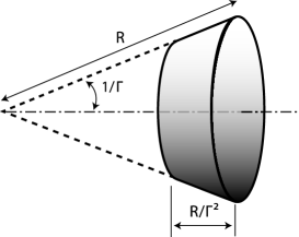
Figure 1.— We consider sources that move along or close enough to the line of sight. Due to relativistic beaming, we can only detect emission within an angle of $1/\Gamma$ with respect to the line of sight. Therefore, unless the jet is very narrow with $\theta_{j}<1/\Gamma$, the effective half-opening angle of the outflow emitting region is $\approx 1/\Gamma$. At a fixed observed time, the emission can only be observed from a lab-frame width of order $R/\Gamma^{2}$, where the distance from the origin of the outflow is $R$. Thus, the region from which emission can be observed (shaded region of this figure) has area $\pi R^{2}/\Gamma^{2}$ and volume $\pi R^{3}/\Gamma^{4}$. We denote this region as the “observed region”. For systems with a different geometry, the emitting region of the outflow, with area $A$ and volume $V$, can be parameterized in terms of the fractions $f_{A}\equiv A/(\pi R^{2}/\Gamma^{2})$ and $f_{V}\equiv V/(\pi R^{3}/\Gamma^{4})$.

We assume a power-law electron energy distribution, which is characterized by a minimal electron LF and a power-law index $p$, assumed to be $p>2$ (the exact value of $p$ will only be relevant when we consider the synchrotron-self-Compton case and the case when $\nu_{m}<\nu_{a}$ – see below). Most of the electrons have energies around this minimal electron LF and they emit at the synchrotron frequency $\nu_{m}$. The synchrotron self-absorption frequency, $\nu_{a}$, could be either above or below $\nu_{m}$. For $\nu_{m}<\nu_{a}$, then the peak frequency is $\nu_{p}=\nu_{a}$, in which case $F_{\nu}\propto\nu^{5/2}$ for $\nu_{m}<\nu<\nu_{a}$ and $F_{\nu}\propto\nu^{2}$ for $\nu<\nu_{m}$. For $\nu_{a}<\nu_{m}$, then $\nu_{p}=\nu_{m}$, in which case $F_{\nu}\propto\nu^{1/3}$ for $\nu_{a}<\nu<\nu_{m}$ and $F_{\nu}\propto\nu^{2}$ for $\nu<\nu_{a}$. Thus, $\nu_{p}=\max(\nu_{a},\nu_{m})$. To take account of these two possibilities, if both $\nu_{a}$ and $\nu_{m}$ can be identified in the spectrum, we define

$$\eta\equiv\left\{\begin{array}[]{ll}{\nu_{m}}/{\nu_{a}}&\textrm{if $\nu_{a}<\nu_{m}$}\\ 1&\textrm{if $\nu_{a}>\nu_{m}$},\\ \end{array}\right.$$ (1)

or $\eta\equiv\nu_{p}/\nu_{a}$. This allows us to consider the most general spectral shape. We assume that the observed peak frequency, $\nu_{p}$, is smaller than the cooling frequency, and we ignore the effect of electron cooling.

In the rest of this section, we will present, without derivation, a summary of the main equations describing relativistic equipartition. These include the estimates of the radius, Lorentz factor and minimal energy. The derivation of these equations, as well as other quantities, is presented in §3.

Energy minimization arguments, which result in a rough equipartition between the electrons and the magnetic field, allow us to constrain four of the five physical parameters of the system. Therefore, we can express the equipartition radius, $R_{eq}$, and minimal total energy, $E_{eq}$, as functions of the observables ($F_{p}$, $d_{L}$, $\nu_{p}$, $\eta$, $z$), the geometrical parameters ($f_{A}$ and $f_{V}$) and one of the physical parameters (we choose the bulk LF of the source) as:

$$R_{eq}\approx(1.7\times 10^{17}{\rm cm})\,\left[F_{p,mJy}^{\frac{8}{17}}\,d_{L,28}^{\frac{16}{17}}\,\nu_{p,10}^{-1}\,\eta^{\frac{35}{51}}\,(1+z)^{-\frac{25}{17}}\right]\,\frac{\Gamma^{\frac{10}{17}}}{f_{A}^{\frac{7}{17}}\,f_{V}^{\frac{1}{17}}},$$ (2)

$$E_{eq}\approx(2.5\times 10^{49}{\rm erg})\,\left[F_{p,mJy}^{\frac{20}{17}}\,d_{L,28}^{\frac{40}{17}}\,\nu_{p,10}^{-1}\,\eta^{\frac{15}{17}}\,(1+z)^{-\frac{37}{17}}\right]\,\frac{f_{V}^{\frac{6}{17}}}{f_{A}^{\frac{9}{17}}\,\Gamma^{\frac{26}{17}}}.$$ (3)

Here, we have used $F_{p,mJy}=F_{\nu,p}/{\rm mJy}$ and, throughout the paper, we use the usual notation $Q_{n}=Q/10^{n}$ in cgs units. For clarity, here and elsewhere, the observed quantities are grouped and written between square brackets to distinguish them clearly from the physical parameters of the system. The next step is to estimate the LF of the source. If it is related to the time since the onset of the relativistic outflow as $t\approx R(1+z)/(2c\Gamma^{2})$, then the radius, bulk LF and minimal total energy are given by:

$$R_{eq}\approx(7.5\times 10^{17}{\rm cm})\,\left[F_{p,mJy}^{\frac{2}{3}}\,d_{L,28}^{\frac{4}{3}}\,\nu_{p,10}^{-\frac{17}{12}}\,\eta^{\frac{35}{36}}\,(1+z)^{-\frac{5}{3}}\,t_{d}^{-\frac{5}{12}}\right]\,f_{A}^{-\frac{7}{12}}\,f_{V}^{-\frac{1}{12}},$$ (4)

$$\Gamma\approx 12\,\left[F_{p,mJy}^{\frac{1}{3}}\,d_{L,28}^{\frac{2}{3}}\,\nu_{p,10}^{-\frac{17}{24}}\,\eta^{\frac{35}{72}}\,(1+z)^{-\frac{1}{3}}\,t_{d}^{-\frac{17}{24}}\right]\,f_{A}^{-\frac{7}{24}}\,f_{V}^{-\frac{1}{24}},$$ (5)

$$E_{eq}\approx(5.7\times 10^{47}{\rm erg})\,\left[F_{p,mJy}^{\frac{2}{3}}\,d_{L,28}^{\frac{4}{3}}\,\nu_{p,10}^{\frac{1}{12}}\,\eta^{\frac{5}{36}}\,(1+z)^{-\frac{5}{3}}\,t_{d}^{\frac{13}{12}}\right]\,f_{A}^{-\frac{1}{12}}\,f_{V}^{\frac{5}{12}},$$ (6)

where the time, $t_{d}$, is measured in days. With $f_{A}=f_{V}=1$ these equations describe the energy within an outflow with a half-opening angle $\theta_{j}=1/\Gamma$ (see Figs. 1 and 2). In §4.1.1 and §4.1.2 we discuss the implications of a narrow jet ($\theta_{j}<1/\Gamma$) and a wider ($\theta_{j}>1/\Gamma$) outflow. We also have not considered here the energy of the electrons that radiate at $\nu_{m}$ when $\nu_{m}<\nu_{a}$, which is discussed in §4.2.1. In addition, a similar analysis can be done for a source for which we know its size but ignore the location of $\nu_{a}$, as discussed in §5.

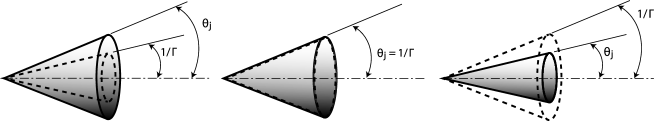
Figure 2.— Different types of relativistic outflows. From left to right: A wide jet, where $\theta_{j}>1/\Gamma$; a jet, where $\theta_{j}\approx 1/\Gamma$, and a narrow jet, where $\theta_{j}<1/\Gamma$. With $f_{A}=f_{V}=1$ all equations in this paper correspond to a jet with $\theta_{j}\approx 1/\Gamma$; however, any general geometry can be considered by using appropriate values for $f_{A}$ and $f_{V}$ (for the case of a narrow and a wide jet see §4.1.1 and §4.1.2).

Alternatively, if a measurement of the synchrotron-self-Compton (SSC) component is available (and securely identified), then one can abandon the energy minimization argument (see §6). In this case, we can express the radius of emission as a function of $\Gamma$ as:

$$R \approx (1\times 10^{17}{\rm cm})\,[5(525)^{p-3}]^{\frac{1}{2(2+p)}}\,\Bigg{[}F_{p,mJy}^{\frac{1}{2}}\,d_{L,28}\,\nu_{p,10}^{-\frac{3+2p}{2(2+p)}}\,\eta^{\frac{5(1+p)}{6(2+p)}}$$ (7)

$$\times(1+z)^{-\frac{5+3p}{2(2+p)}}\,\left(\frac{F_{\nu,p}}{F_{\nu}^{SSC}}\right)^{\frac{1}{2(2+p)}}\,\left(\frac{\nu_{p}}{\nu_{obs}^{SSC}}\right)^{\frac{p-1}{4(2+p)}}\Bigg{]}\,f_{A}^{-\frac{1+p}{2(2+p)}}\,\Gamma^{\frac{1+p}{2(2+p)}},$$

where $\nu_{obs}^{SSC}$ and $F_{\nu}^{SSC}$ are the measured frequency and specific flux of the SSC component, and the measured frequency is above the SSC peak. In a similar way as done above, relating the bulk LF of the source to the time since the onset of the relativistic explosion allows us to determine $R$ (and all other physical parameters) only as function of observables. Here, we show $R$ and $\Gamma$:

$$R \approx (1\times 10^{17}{\rm cm})\,C_{1}^{\frac{2}{7+3p}}\,C_{2}^{\frac{2(1+p)}{7+3p}}\,\Bigg{[}F_{p,mJy}^{\frac{2(2+p)}{7+3p}}\,d_{L,28}^{\frac{4(2+p)}{7+3p}}\,\nu_{p,10}^{-\frac{2(3+2p)}{7+3p}}\,\eta^{\frac{10(1+p)}{3(7+3p)}}$$ (8)

$$\times(1+z)^{-\frac{9+5p}{7+3p}}\,t_{d}^{-\frac{1+p}{7+3p}}\,\left(\frac{F_{\nu,p}}{F_{\nu}^{SSC}}\right)^{\frac{2}{7+3p}}\,\left(\frac{\nu_{p}}{\nu_{obs}^{SSC}}\right)^{\frac{p-1}{7+3p}}\Bigg{]}\,f_{A}^{-\frac{2(1+p)}{7+3p}},$$

$$\Gamma \approx C_{1}^{\frac{1}{7+3p}}\,C_{2}^{\frac{4(2+p)}{7+3p}}\,\Bigg{[}F_{p,mJy}^{\frac{2+p}{7+3p}}\,d_{L,28}^{\frac{2(2+p)}{7+3p}}\,\nu_{p,10}^{-\frac{3+2p}{7+3p}}\,\eta^{\frac{5(1+p)}{3(7+3p)}}$$ (9)

$$\times(1+z)^{-\frac{1+p}{7+3p}}\,t_{d}^{-\frac{2(2+p)}{7+3p}}\,\left(\frac{F_{\nu,p}}{F_{\nu}^{SSC}}\right)^{\frac{1}{7+3p}}\,\left(\frac{\nu_{p}}{\nu_{obs}^{SSC}}\right)^{\frac{p-1}{2(7+3p)}}\Bigg{]}f_{A}^{-\frac{1+p}{7+3p}},$$

where $C_{1}\approx 5(525)^{p-3}$ and $C_{2}\approx 4.4$, and the rest of the parameters can be found in the Appendix, including the total energy in electrons and magnetic field.

3. Derivation of the radius estimate and the minimal total energy

A synchrotron emitting system is characterized by three equations: the synchrotron frequency, the synchrotron flux and the black-body flux. The observed synchrotron frequency is

$$\nu_{p}=\frac{eB\gamma_{e}^{2}\Gamma}{2\pi m_{e}c(1+z)},$$ (10)

where $e$ is the electron charge, $m_{e}$ is the electron mass, $c$ is the speed of light and $z$ is the redshift. The observed synchrotron maximum specific flux, at $\nu_{p}$, is

$$F_{\nu,p}=\frac{\sqrt{3}e^{3}BN_{e}\Gamma^{3}(1+z)}{\pi d_{L}^{2}m_{e}c^{2}},$$ (11)

where we have used the fact that the emission is beamed into a solid angle of $\pi/\Gamma^{2}$. This expression is different than eq. (5) of Sari et al. (1998; see, also, Kumar & Narayan 2009) that uses $N_{e,iso}$, the isotropic equivalent number of electrons, rather than $N_{e}$, the number of electrons within the observed region ($N_{e,iso}=4\Gamma^{2}N_{e}$). This additional factor of $4$ introduces small corrections when taking the Newtonian limit ($\Gamma=1$): Eqs. (21), (25), (27), (28), (29) and (30), should be multiplied by $4^{1/17}$, $4^{11/17}$, $4^{{1/(13+2p)}}$, $4^{{11/(13+2p)}}$, $4^{2/7}$ and $4^{4/7}$, respectively.

The black-body specific flux, at frequency $\nu\leq\nu_{a}$, is given by

$$F_{\nu,BB}=2\nu^{2}(1+z)^{3}\Gamma m_{e}\gamma_{e}\frac{A}{d_{L}^{2}},$$ (12)

where $A=f_{A}\pi R^{2}/\Gamma^{2}$ and we have used an equivalent effective black-body temperature, $kT$, as the energy of the electrons radiating at the peak, $kT\approx m_{e}c^{2}\gamma_{e}$. The flux at $\nu_{a}$ is:

$$F_{\nu_{a},BB}=F_{\nu,p}\eta^{-\frac{1}{3}}.$$ (13)

Using eqs. (10)–(13) we can solve for three of the five physical parameters, $\gamma_{e}$, $N_{e}$ and $B$, as functions of the observables ($F_{p}$, $d_{L}$, $\nu_{p}$, $\eta$, $z$), the remaining two physical parameters ($R$ and $\Gamma$), and the geometrical parameters ($f_{A}$ and $f_{V}$):

$$\gamma_{e}=\frac{3F_{\nu,p}d_{L}^{2}\eta^{\frac{5}{3}}\Gamma}{2\pi\nu_{p}^{2}(1+z)^{3}m_{e}f_{A}R^{2}}\approx 525\,\left[F_{p,mJy}\,d_{L,28}^{2}\,\nu_{p,10}^{-2}\,\eta^{\frac{5}{3}}\,(1+z)^{-3}\right]\,\frac{\Gamma}{f_{A}\,R_{17}^{2}},$$ (14)

$$N_{e}=\frac{9cF_{\nu,p}^{3}d_{L}^{6}\eta^{\frac{10}{3}}}{8\sqrt{3}\pi^{2}e^{2}m_{e}^{2}\nu_{p}^{5}(1+z)^{8}f_{A}^{2}R^{4}}\approx 1\times 10^{54}\,\left[F_{p,mJy}^{3}\,d_{L,28}^{6}\,\nu_{p,10}^{-5}\,\eta^{\frac{10}{3}}\,(1+z)^{-8}\right]\,\frac{1}{f_{A}^{2}\,R_{17}^{4}},$$ (15)

$$B=\frac{8\pi^{3}m_{e}^{3}c\nu_{p}^{5}(1+z)^{7}f_{A}^{2}R^{4}}{9eF_{\nu,p}^{2}d_{L}^{4}\eta^{\frac{10}{3}}\Gamma^{3}}\approx(1.3\times 10^{-2}\,{\rm G})\,\left[F_{p,mJy}^{-2}\,d_{L,28}^{-4}\,\nu_{p,10}^{5}\,\eta^{-\frac{10}{3}}\,(1+z)^{7}\right]\,\frac{f_{A}^{2}\,R_{17}^{4}}{\Gamma^{3}}.$$ (16)

The energy in electrons within the observed region is

$$E_{e} = N_{e}m_{e}c^{2}\gamma_{e}\Gamma=\frac{27c^{3}F_{\nu,p}^{4}d_{L}^{8}\eta^{5}\Gamma^{2}}{16\sqrt{3}\pi^{3}e^{2}m_{e}^{2}\nu_{p}^{7}(1+z)^{11}f_{A}^{3}R^{6}}$$ (17)

$$\approx (4.4\times 10^{50}{\rm erg})\,\Big{[}F_{p,mJy}^{4}\,d_{L,28}^{8}\,\nu_{p,10}^{-7}\,\eta^{5}\,(1+z)^{-11}\Big{]}\,\frac{\Gamma^{2}}{f_{A}^{3}\,R_{17}^{6}},$$

while the energy in the magnetic field is

$$E_{B} = \frac{(B\Gamma)^{2}}{8\pi}V=\frac{8\pi^{6}m_{e}^{6}c^{2}\nu_{p}^{10}(1+z)^{14}f_{A}^{4}f_{V}R^{11}}{81e^{2}F_{\nu,p}^{4}d_{L}^{8}\eta^{\frac{20}{3}}\Gamma^{8}}$$ (18)

$$\approx (2.1\times 10^{46}{\rm erg})\,\left[F_{p,mJy}^{-4}\,d_{L,28}^{-8}\,\nu_{p,10}^{10}\,\eta^{-\frac{20}{3}}\,(1+z)^{14}\right]\,\frac{f_{A}^{4}\,f_{V}\,R_{17}^{11}}{\Gamma^{8}},$$

where $V=f_{V}\pi R^{3}/\Gamma^{4}$.

Eqs. (14)–(18) are reduced to the Newtonian case for $\Gamma=f_{A}=1$ (note, however, that additional factors of powers of 4, mentioned following eq. (11), should be added, and that $f_{V}=4/3$ in the spherical Newtonian case). In the Newtonian analysis $\eta=1$ is generally used. According to the classical Newtonian equipartition argument, we minimize the total energy to obtain the Newtonian equipartition radius and minimal total energy in terms of the observables:

$$R_{N} \approx (1.7\times 10^{17}{\rm cm})\,\left[F_{p,mJy}^{\frac{8}{17}}\,d_{L,28}^{\frac{16}{17}}\,\nu_{p,10}^{-1}\,\eta^{\frac{35}{51}}\,(1+z)^{-\frac{25}{17}}\right],$$

$$E_{N} \approx (2.5\times 10^{49}{\rm erg})\,\left[F_{p,mJy}^{\frac{20}{17}}\,d_{L,28}^{\frac{40}{17}}\,\nu_{p,10}^{-1}\,\eta^{\frac{15}{17}}\,(1+z)^{-\frac{37}{17}}\right].$$ (19)

Generalizing to the relativistic non-spherical symmetric case we can express, now, the total energy using $R_{N}$ and $E_{N}$ as:

$$E=E_{e}+E_{B}=E_{N}\left(\frac{f_{V}^{\frac{6}{17}}}{f_{A}^{\frac{9}{17}}\Gamma^{\frac{26}{17}}}\right)\left[\frac{11}{17}\left(\frac{R}{R_{eq}}\right)^{-6}+\frac{6}{17}\left(\frac{R}{R_{eq}}\right)^{11}\right].$$ (20)

$R_{eq}$ (in the Newtonian case $R_{eq}=R_{N}$) is the relativistic equipartition radius:

$$R_{eq}\equiv\,R_{N}\,\frac{\Gamma^{\frac{10}{17}}}{f_{A}^{\frac{7}{17}}\,f_{V}^{\frac{1}{17}}}\approx(1.7\times 10^{17}{\rm cm})\,\left[F_{p,mJy}^{\frac{8}{17}}\,d_{L,28}^{\frac{16}{17}}\,\nu_{p,10}^{-1}\,\eta^{\frac{35}{51}}\,(1+z)^{-\frac{25}{17}}\right]\,\frac{\Gamma^{\frac{10}{17}}}{f_{A}^{\frac{7}{17}}\,f_{V}^{\frac{1}{17}}}.$$ (21)

The total energy is minimized with respect to $R$ at $R_{eq}$, with $E_{B}\approx(6/11)E_{e}$. Since the total energy is a very strong function of radius, $R_{eq}$ provides a robust estimate of $R$, unless we allow the total energy to be significantly higher than the minimal allowed total energy.

Examination of eq. (21) reveals that $R_{eq}$ varies only weakly with variation in the geometry. Specifically, it is insensitive to the volume filling factor, $f_{V}$, and it depends only weakly on the area filling factor $f_{A}$. A considerable deviation from spherical symmetry is required to affect the radius estimate. Moreover, $R_{eq}$ increases with $\Gamma$, thus the application of the Newtonian estimate to an ultrarelativistic source results in a significant underestimate of its radius.

In the relativistic case, the total energy, eq. (20), depends on two unknowns: $R$ and $\Gamma$. For any given $\Gamma$ the energy is minimized at $R=R_{eq}$. However, if we choose $R=R_{eq}(\Gamma)$ then the value in square brackets of eq. (20) is just unity and $E\propto\Gamma^{-26/17}$ Hence there is no global minimum for this function and we must determine $\Gamma$ independently. We need now another relation that will enable us to express $\Gamma$ as a function of $R$. To obtain this relation we introduce an extra observable, $t$, the time, in the observer frame, since the onset of the relativistic outflow. In most astrophysical scenarios $\Gamma$ evolves on a time scale comparable to, or longer than, $t$ and:

$$t\approx\frac{R(1-\beta)(1+z)}{\beta c},$$ (22)

where $\beta$ is the velocity of the outflow at observer time $t$. If the time of the onset of the outflow is known then a single measurement of the synchrotron spectrum is enough and eqs. (21) and (22) are solved simultaneously to determine $R$ and $\Gamma$. In the extreme relativistic limit $\Gamma\gg 1$, $t\approx R(1+z)/(2c\Gamma^{2})$ and we find a radius

$$R_{eq}\approx(7.5\times 10^{17}{\rm cm})\,\left[F_{p,mJy}^{\frac{2}{3}}\,d_{L,28}^{\frac{4}{3}}\,\nu_{p,10}^{-\frac{17}{12}}\,\eta^{\frac{35}{36}}\,(1+z)^{-\frac{5}{3}}\,t_{d}^{-\frac{5}{12}}\right]\,f_{A}^{-\frac{7}{12}}\,f_{V}^{-\frac{1}{12}},$$ (23)

and a bulk LF given by

$$\Gamma\approx 12\,\left[F_{p,mJy}^{\frac{1}{3}}\,d_{L,28}^{\frac{2}{3}}\,\nu_{p,10}^{-\frac{17}{24}}\,\eta^{\frac{35}{72}}\,(1+z)^{-\frac{1}{3}}\,t_{d}^{-\frac{17}{24}}\right]\,f_{A}^{-\frac{7}{24}}\,f_{V}^{-\frac{1}{24}},$$ (24)

where $t_{d}$ is the time measured in days.

If the onset of the outflow is unknown, then we need at least two epochs, $t_{1}$ and $t_{2}$, at which $F_{\nu,p}$ and $\nu_{p}$ (and $\nu_{a}$ if it is not the peak frequency) are measured. If $\Gamma(t_{1})\sim\Gamma(t_{2})$, we solve eqs. (21) and (22) for $R(t_{2})$ and $R(t_{1})$ and $t_{2}$ and $t_{1}$. However, $\Gamma$ may evolve on a time scale comparable to $t$. Therefore if $t_{2}\gg t_{1}$ it is possible that $\Gamma(t_{1})\nsim\Gamma(t_{2})$. This case is identified if the above procedure results in $R(t_{2})\gg R(t_{1})$. Then $t_{2}-t_{1}\sim t$ and $R(t_{2})-R(t_{1})\sim R$, and we can approximate the solution at $t_{2}$ using $t_{2}\approx t$. In this case the solution of $R(t_{1})$ cannot be trusted.

Substitution of $R_{eq}$ into eq. (20) yields the absolute minimal total energy of the system. This energy accounts only for the electrons that radiate at $\nu_{p}$ and for the corresponding magnetic field. For both components we consider only the energy within the observed region:

$$E_{eq}=E_{N}\,\frac{f_{V}^{\frac{6}{17}}}{f_{A}^{\frac{9}{17}}\,\Gamma^{\frac{26}{17}}}\approx(2.5\times 10^{49}{\rm erg})\,\left[F_{p,mJy}^{\frac{20}{17}}\,d_{L,28}^{\frac{40}{17}}\,\nu_{p,10}^{-1}\,\eta^{\frac{15}{17}}\,(1+z)^{-\frac{37}{17}}\right]\,\frac{f_{V}^{\frac{6}{17}}}{f_{A}^{\frac{9}{17}}\,\Gamma^{\frac{26}{17}}}.$$ (25)

This lower limit decreases with $\Gamma$, and, therefore, it is less stringent for relativistic sources. This is driven mostly by the increased beaming, and thus the reduced area and volume within an angle of $\sim 1/\Gamma$. In the relativistic limit, $\Gamma\gg 1$, we can use eq. (24) to obtain:

$$E_{eq}\approx(5.7\times 10^{47}{\rm erg})\,\left[F_{p,mJy}^{\frac{2}{3}}\,d_{L,28}^{\frac{4}{3}}\,\nu_{p,10}^{\frac{1}{12}}\,\eta^{\frac{5}{36}}\,(1+z)^{-\frac{5}{3}}\,t_{d}^{\frac{13}{12}}\right]\,f_{A}^{-\frac{1}{12}}\,f_{V}^{\frac{5}{12}}.$$ (26)

The radius $R_{eq}$ that was obtained by minimizing the energy and assuming equipartition is a robust estimate even if the system is out of equipartition. We define the microphysical parameters, $\epsilon_{e}$ and $\epsilon_{B}$, as the fractions of the total energy in electrons and magnetic field, respectively. The energy is minimal for $\epsilon_{B}/\epsilon_{e}\approx 6/11$. The ratio, $\epsilon\equiv(\epsilon_{B}/\epsilon_{e})/(6/11)$, parameterizes the deviation from equipartition. The radius is multiplied by $\epsilon^{1/17}$ for the Newtonian case, and by a factor of $\epsilon^{1/12}$ (and consequently $\Gamma$ is multiplied by a factor of $\epsilon^{1/24}$) in the relativistic ($\Gamma\gg 1$) case. While the emission radius depends extremely weakly on $\epsilon$, the total energy is a strong function of $\epsilon$ and deviations from equipartition increase significantly the overall energy budget. The energy is larger than the minimal total energy by $\approx(11/17)\epsilon^{-6/17}+(6/17)\epsilon^{11/17}$ in the Newtonian case and by $\approx(11/17)\epsilon^{-5/12}+(6/17)\epsilon^{7/12}$ if the system is relativistic.

4. The minimal (equipartition) energy

Eq. (25) provides an absolute lower limit to the energy of the system. This expression includes the energy of the electrons emitting at $\nu_{p}$ and the corresponding magnetic field. Both terms are calculated within the observed region of half-opening angle of $\sim 1/\Gamma$. We examine several cases in which additional energy is “hidden” in the system and is not observed directly, but it influences, of course, the overall energy budget. However, before doing so we consider the effect of the geometrical factors on the system.

4.1. Geometrical effects

The effect of deviation from spherical geometry is opposite for $f_{A}$ and $f_{V}$, for both the Newtonian, $E_{eq}\propto f_{A}^{-9/17}f_{V}^{6/17}$, and the relativistic, $E_{eq}\propto f_{A}^{-1/12}f_{V}^{5/12}$, cases; see eqs. (25) and (26), respectively.

4.1.1 Narrow jets

A particularly interesting geometric effect is the one in a relativistic narrow jet with half-opening angle $\theta_{j}$ that is smaller than $1/\Gamma$ (see Fig. 2). In this case we define $f_{\theta}\equiv(\theta_{j}\Gamma)^{2}$ and both geometric factors satisfy: $f_{A}=f_{V}=f_{\theta}$. Substituting these values into eqs. (23), (24) and (26) we find $R\propto f_{\theta}^{-2/3}$, $\Gamma\propto f_{\theta}^{-1/3}$ and $E_{eq}\propto f_{\theta}^{1/3}$. Since $f_{\theta}<1$, this implies that the radius and bulk LF of a narrow jet will be larger than in the case with $f_{A}=f_{V}=1$; however, the resulting minimal energy will be smaller. Specifically, these quantities scale with $\theta_{j}$ as $R\propto\theta_{j}^{-4/5}$, $\Gamma\propto\theta_{j}^{-2/5}$ and $E_{eq}\propto\theta_{j}^{2/5}$. Thus, a jet narrower than $1/\Gamma$ requires lower energy to produce the observed emission (although the decrease in energy is small given the weak $\theta_{j}$-dependence of the minimal energy). The reason for this effect is not trivial (as there are competing effects), but the main driver is the reduction in the area, which reduces $B$ and leads to a significant increase of $R_{eq}$ and $\Gamma$. This results in a lower $E_{eq}$ than in the $f_{A}=f_{V}=1$ case, see eq. (25).

4.1.2 Wide outflows

The outflow’s half-opening angle could be larger than $1/\Gamma$ (see Fig. 2). In this case the overall energy of the source is larger, as additional energy at the region $\theta_{j}>1/\Gamma$ has negligible contribution to the observed emission . The flow will carry an energy larger than the one calculated in eq. (25), with $f_{A}=f_{V}=1$, by a factor of $4\Gamma^{2}(1-\cos\theta_{j})$. The “true” energy can be determined only if an independent estimate of the jet opening angle is available (such as in GRBs, when a “jet break” takes place and $\theta_{j}$ can be estimated, e.g., Sari et al. 1999).

4.2. Unaccounted-for energy

4.2.1 Electrons that radiate at $\nu_{m}$

Above we considered only the electrons that radiate at $\nu_{p}$. These electrons are likely to carry most of the relativistic electron energy if $\nu_{p}=\nu_{m}$. However, if $\nu_{m}<\nu_{a}$ most of the electrons’ energy is carried by the electrons with the minimal Lorentz factor, $\gamma_{m}$ (and whose emission is self-absorbed). In this case the electrons’ energy will be larger than that of eq. (17) (with $\eta=1$), by a factor of $(\gamma_{m}/\gamma_{e})^{2-p}$, where $p$ is the electron energy distribution power-law and $p>2$. In rare cases $\nu_{m}$ can be identified in the spectrum. This can be done if spectra at different epochs are available and one observes a transition in the spectrum from $F_{\nu}\propto\nu^{2}$ to $F_{\nu}\propto\nu^{5/2}$. In these cases $(\gamma_{m}/\gamma_{e})^{2-p}=(\nu_{m}/\nu_{a})^{(2-p)/2}$, so the radius estimate is hardly modified, since it is only multiplied by $(\nu_{m}/\nu_{a})^{(2-p)/34}$ in eq. (21) (with $\eta=1$). The total minimal energy is somewhat increased, since it is multiplied by $(\nu_{m}/\nu_{a})^{11(2-p)/34}$ in eq. (25) (with $\eta=1$). In the most common case where $\nu_{m}$ is not measured it must be evaluated theoretically. This can be done if the electrons are known to be accelerated by a shock with LF similar to that of the source, $\Gamma$. In that case $\gamma_{m}=\chi_{e}(\Gamma-1)$ where $\chi_{e}=\frac{p-2}{p-1}\epsilon_{e}\frac{m_{p}}{m_{e}}$ and $\epsilon_{e}$ is the fraction of the protons energy that goes into electrons and $m_{p}$ is the proton mass (if $\gamma_{m}$ is found to be $\gamma_{m}<2$, then one should use $\gamma_{m}=2$). With this, and following the same procedure as above of setting $E_{B}\approx(6/11)E_{e}$, the radius where the energy is minimal becomes

$$R_{eq} \approx (1\times 10^{17}{\rm cm})\,[21.8(525)^{p-1}]^{\frac{1}{13+2p}}\,\chi_{e}^{\frac{2-p}{13+2p}}\,\Big{[}F_{p,mJy}^{\frac{6+p}{13+2p}}\,d_{L,28}^{\frac{2(p+6)}{13+2p}}$$ (27)

$$\times\,\nu_{p,10}^{-1}\,(1+z)^{-\frac{19+3p}{13+2p}}\Big{]}\,f_{A}^{-\frac{5+p}{13+2p}}\,f_{V}^{-\frac{1}{13+2p}}\,\Gamma^{\frac{p+8}{13+2p}}\,(\Gamma-1)^{\frac{2-p}{13+2p}}.$$

The corresponding minimal total energy within the observed region is:

$$E_{eq} \approx (1.3\times 10^{48}{\rm erg})\,[21.8]^{-\frac{2(p+1)}{13+2p}}\,[(525)^{p-1}\chi_{e}^{2-p}]^{\frac{11}{13+2p}}\,\Big{[}F_{p,mJy}^{\frac{14+3p}{13+2p}}\,d_{L,28}^{\frac{2(3p+14)}{13+2p}}$$ (28)

$$\times\,\nu_{p,10}^{-1}\,(1+z)^{-\frac{27+5p}{13+2p}}\Big{]}\,f_{A}^{-\frac{3(p+1)}{13+2p}}\,f_{V}^{\frac{2(p+1)}{13+2p}}\,\Gamma^{-\frac{5p+16}{13+2p}}\,(\Gamma-1)^{-\frac{11(p-2)}{13+2p}}.$$

The last two expressions reduce to eqs. (21) and (25) with $\eta=1$ for $p=2$ (when all electrons carry a similar amount of energy). For the Newtonian case, $\gamma_{m}=2$ and $p=3$, one obtains the solution found by Chevalier (1998).

4.2.2 Hot protons

If the source contains protons it is reasonable to expect that these take a significant share of the total internal and bulk energy. For example, observations indicate that in shock heated gas (for example, in GRB afterglows, see, e.g., Panaitescu & Kumar 2002) most of the energy is carried by hot protons. The exact fraction of the total energy carried by other components is unknown, but these observations suggest that the fraction carried by electrons, $\epsilon_{e}$, is typically $\sim 0.1$ in relativistic shocks and lower in Newtonian shocks. Using this parameterization, the energy carried by the hot protons is $E_{p}\approx E_{e}/\epsilon_{e}$. This implies a total matter energy of $E_{e}+E_{p}=\xi E_{e}$, where $\xi\equiv 1+\epsilon_{e}^{-1}$. Similarly, the parameters at which the energy is minimal are found by setting $E_{B}\approx(6/11)\xi E_{e}$. The radius estimate is hardly modified, since it is only multiplied by $\xi^{1/17}$, $\xi^{1/12}$ and $\xi^{1/(13+2p)}$ in eqs. (21), (23) and (27), respectively. The total minimal energy is somewhat increased, since it is multiplied by $\xi^{11/17}$, $\xi^{7/12}$ and $\xi^{11/(13+2p)}$ in eqs. (25), (26) and (28), respectively.

5. Systems with measured $R$ but unknown self-absorption frequency

.

There are cases, especially for Galactic and local universe sources, in which we can resolve and measure the source’s size on the sky and determine $R\psi=\theta_{obs}d_{A}$, where $\psi\equiv\min(1/\Gamma,\theta_{j})$, $\theta_{obs}$ is the half-angular extent of the source and $d_{A}=d_{L}(1+z)^{-2}$ is the angular distance. However, for these sources we do not always have a measurement of $\nu_{a}$. We can still estimate a minimal total energy carried by the magnetic field and by electrons that radiate at the observed frequency $\nu$ at a flux $F_{\nu}$. This was first done in the Newtonian case by Burbidge (1959; see, e.g., Nakar et al. 2005, for a recent example) and the relativistic case, without considering any geometrical factors, was discussed in Dermer & Atoyan (2004; see also Dermer & Menon 2009). Determining the LF of electrons radiating at $\nu$ with (10) and the number of radiating electrons within $1/\Gamma$ with (11), we can determine the total energy of the system. It is minimized once $E_{B}\approx(3/4)E_{e}$, which yields an equipartition magnetic field (see, e.g., Dermer & Menon 2009)

$$B_{eq}\approx(5\times 10^{-3}{\rm G})\,\left[F_{\nu,mJy}^{\frac{2}{7}}\,\left(\frac{d_{L}}{10{\rm kpc}}\right)^{-\frac{2}{7}}\,\nu_{10}^{\frac{1}{7}}\,(1+z)^{\frac{11}{7}}\,\left(\frac{\theta_{obs}}{10{\rm mas}}\right)^{-\frac{6}{7}}\right]\,f_{V}^{-\frac{2}{7}}\,\psi^{\frac{6}{7}}\,\Gamma^{-\frac{1}{7}}.$$ (29)

The energy in the magnetic field can be determined with $B_{eq}$, and the total minimal energy within the observed region, which is given by $E_{e}+E_{B}=(7/3)E_{B}$, is

$$E_{eq}\approx(2.8\times 10^{40}{\rm erg})\,\left[F_{\nu,mJy}^{\frac{4}{7}}\,\left(\frac{d_{L}}{10{\rm kpc}}\right)^{\frac{17}{7}}\,\nu_{10}^{\frac{2}{7}}\,(1+z)^{-\frac{20}{7}}\,\left(\frac{\theta_{obs}}{10{\rm mas}}\right)^{\frac{9}{7}}\right]\,f_{V}^{\frac{3}{7}}\,\psi^{-\frac{9}{7}}\,\Gamma^{-\frac{16}{7}},$$ (30)

where $F_{\nu,mJy}=F_{\nu}/mJy$. For these nearby sources we usually have the time of the onset of the outflow and can estimate $\Gamma$. This allows us to use (30) to estimate the absolute minimum total energy.

6. Synchrotron-self-Compton emission

If synchrotron-self-Compton (SSC) emission is also observed, then there is no need to minimize the total energy. This introduces two additional observables that allow us to determine all parameters of the system without the need of minimizing the total energy. This was done by Chevalier & Fransson (2006) and later by Katz (2012) for the Newtonian case. Here, we extend these estimates to the relativistic case, again, following the spirit of Kumar & Narayan (2009; see also Dermer & Atoyan 2004). If the synchrotron emission peaks in the radio band and the SSC observed emission is in the X-rays, then it is safe to assume, as we do in the following, that the Klein-Nishina effects can be neglected.

The SSC peak frequency, $\nu_{p}^{SSC}$, and the ratio of the synchrotron to the SSC luminosities are

$$\nu_{p}^{SSC}\approx\nu_{p}\gamma_{e}^{2},$$ (31)

and

$$\frac{B^{2}/8\pi}{U_{ph}}\approx\frac{\nu_{p}F_{\nu,p}}{\nu_{p}^{SSC}F_{\nu,p}^{SSC}},$$ (32)

where $U_{ph}$ is the photon energy density (in the co-moving frame) and $F_{\nu,p}^{SSC}$ is the SSC peak flux. Note that eq. (31) is correct for both $\nu_{a}<\nu_{m}$ or $\nu_{m}<\nu_{a}$, since $\gamma_{e}$ corresponds to the electrons radiating at $\nu_{p}=\max(\nu_{a},\nu_{m})$. The photon energy density can be approximated as $U_{ph}=\frac{\nu_{p}F_{\nu,p}}{\Gamma^{2}c}\frac{d_{L}^{2}}{R^{2}}$.

Consider an observed SSC frequency $\nu_{obs}^{SSC}$, such that $\nu_{p}^{SSC}<\nu_{obs}^{SSC}$, with observed flux $F_{\nu}^{SSC}$. These observations are related to the peak of the SSC component as

$$F_{\nu}^{SSC}=F_{\nu,p}^{SSC}\left(\frac{\nu_{obs}^{SSC}}{\nu_{p}^{SSC}}\right)^{-\frac{p-1}{2}}.$$ (33)

Using eqs. (14), (16), and (31)–(33), we can solve for the radius of emission

$$R \approx (1\times 10^{17}{\rm cm})\,[5(525)^{p-3}]^{\frac{1}{2(2+p)}}\,\Bigg{[}F_{p,mJy}^{\frac{1}{2}}\,d_{L,28}\,\nu_{p,10}^{-\frac{3+2p}{2(2+p)}}\,\eta^{\frac{5(1+p)}{6(2+p)}}$$ (34)

$$\times(1+z)^{-\frac{5+3p}{2(2+p)}}\,\left(\frac{F_{\nu,p}}{F_{\nu}^{SSC}}\right)^{\frac{1}{2(2+p)}}\,\left(\frac{\nu_{p}}{\nu_{obs}^{SSC}}\right)^{\frac{p-1}{4(2+p)}}\Bigg{]}\,f_{A}^{-\frac{1+p}{2(2+p)}}\,\Gamma^{\frac{1+p}{2(2+p)}}.$$

This expression and eq. (22) allow us to determine the radius of emission and $\Gamma$ of the source. We can then substitute the obtained values for $R$ and $\Gamma$ in eqs. (14)-(18) and obtain all physical parameters of the emitting region. In the extreme relativistic limit $\Gamma\gg 1$, we can solve for all these parameters analytically (see the Appendix for these expressions).

Finally, we note that for $\Gamma=1$ and $p=3$, eq. (34) reduces to the radius estimate in Katz (2012) for the Newtonian case, within a factor of $\sim 2$. This small discrepancy appears simply because our expression for the synchrotron frequency, eq. (10), is larger than the one used by Katz (2012) by this same factor.

7. Summary

We have extended the equipartition arguments of Newtonian synchrotron sources in spherical geometry to include relativistic sources in general geometry. This enables to derive robust estimates of the radius and of the minimal total energy of the emitting region of a large variety of synchrotron transient sources. It also enables to quantify the effect of the, typically unknown, geometry on the robustness of these estimates.

We find that in the relativistic case the estimate of the emission radius is increased by a factor of $\Gamma^{10/17}$ compared with the Newtonian case. The lower limit on the energy (within a region of $\sim 1/\Gamma$) is lower by $\Gamma^{-26/17}$ compared with the Newtonian one. Therefore, using the Newtonian formalism for a relativistic source underestimates (overestimates) the emission radius (lower limit on the energy). We show that in order to find if relativistic corrections are needed, and to estimate $\Gamma$, at least two epochs of measurements are needed, or alternatively the time since the onset of the outflow should be known.

The collimation of relativistic sources affects the energy lower limit. Throughout the paper we considered an observed region of $\sim 1/\Gamma$; however, considering a source with half-opening angle smaller (larger) than $1/\Gamma$ yields smaller (higher) lower limits. A wider jet involves additional energy that we do not observe directly as it is beamed elsewhere, while the reason why a narrower jet requires lower energy is less trivial and is discussed above.

The energy estimates discussed above involve the minimal energy (of the electrons and the magnetic field) required to produce the observed radiation. However, additional components in which energy is “hidden” may exist in the system. These include: 1. The extra energy carried by electrons with minimal Lorentz Factor $\gamma_{m}$ and whose synchrotron frequency $\nu_{m}$ is self-absorbed, such that $\nu_{m}<\nu_{a}$, and 2. the energy carried by protons, if they are present in the source. We consider their possible effect on the total energy required. We find that these extra sources of energy hardly change the emission radius, while the total minimal energy is increased.

Finally, we extend the Newtonian equipartition formalism to relativistic sources in two other scenarios. First, for nearby sources, where we are able to identify the angular size of the source on the sky, but the self-absorption frequency is not identified. Second, for when a synchrotron-self-Compton component is identified, in addition to the synchrotron self-absorption, and there are two additional observables that enable us to directly determine all parameters of the emitting region. Overall we find that relativistic corrections can be important and that using the Newtonian formula for a relativistic source would lead to significantly inaccurate results.

Appendix

If a reliable measurement of the SSC flux is available, then there is no need to minimize the total energy; all parameters of the emitting region can be uniquely determined (see §6). In the extreme relativistic limit $\Gamma\gg 1$, eq. (22) is $t\approx R(1+z)/(2c\Gamma^{2})$, and we can solve for all these parameters analytically as follows. The radius of emission will be given by eq. (34) as

$$R \approx (1\times 10^{17}{\rm cm})\,C_{1}^{\frac{2}{7+3p}}\,C_{2}^{\frac{2(1+p)}{7+3p}}\,\Bigg{[}F_{p,mJy}^{\frac{2(2+p)}{7+3p}}\,d_{L,28}^{\frac{4(2+p)}{7+3p}}\,\nu_{p,10}^{-\frac{2(3+2p)}{7+3p}}\,\eta^{\frac{10(1+p)}{3(7+3p)}}$$ (A1)

$$\times(1+z)^{-\frac{9+5p}{7+3p}}\,t_{d}^{-\frac{1+p}{7+3p}}\,\left(\frac{F_{\nu,p}}{F_{\nu}^{SSC}}\right)^{\frac{2}{7+3p}}\,\left(\frac{\nu_{p}}{\nu_{obs}^{SSC}}\right)^{\frac{p-1}{7+3p}}\Bigg{]}\,f_{A}^{-\frac{2(1+p)}{7+3p}},$$

and $\Gamma$ will be given by

$$\Gamma \approx C_{1}^{\frac{1}{7+3p}}\,C_{2}^{\frac{4(2+p)}{7+3p}}\,\Bigg{[}F_{p,mJy}^{\frac{2+p}{7+3p}}\,d_{L,28}^{\frac{2(2+p)}{7+3p}}\,\nu_{p,10}^{-\frac{3+2p}{7+3p}}\,\eta^{\frac{5(1+p)}{3(7+3p)}}$$ (A2)

$$\times(1+z)^{-\frac{1+p}{7+3p}}\,t_{d}^{-\frac{2(2+p)}{7+3p}}\,\left(\frac{F_{\nu,p}}{F_{\nu}^{SSC}}\right)^{\frac{1}{7+3p}}\,\left(\frac{\nu_{p}}{\nu_{obs}^{SSC}}\right)^{\frac{p-1}{2(7+3p)}}\Bigg{]}f_{A}^{-\frac{1+p}{7+3p}},$$

where $C_{1}\approx 5(525)^{p-3}$ and $C_{2}\approx 4.4$. With these two expressions, the rest of the parameters can be determined by substituting them in eqs. (14)-(18) as follows:

$$\gamma_{e} \approx 525C_{1}^{-\frac{3}{7+3p}}\,C_{2}^{\frac{4}{7+3p}}\,\Bigg{[}F_{p,mJy}^{\frac{1}{7+3p}}\,d_{L,28}^{\frac{2}{7+3p}}\,\nu_{p,10}^{-\frac{5}{7+3p}}\,\eta^{\frac{20}{3(7+3p)}}$$ (A3)

$$\times(1+z)^{-\frac{4}{7+3p}}\,t_{d}^{-\frac{2}{7+3p}}\,\left(\frac{F_{\nu,p}}{F_{\nu}^{SSC}}\right)^{-\frac{3}{7+3p}}\,\left(\frac{\nu_{p}}{\nu_{obs}^{SSC}}\right)^{\frac{3(1-p)}{2(7+3p)}}\Bigg{]}f_{A}^{-\frac{4}{7+3p}},$$

$$N_{e} \approx 1\times 10^{54}\,C_{1}^{-\frac{8}{7+3p}}\,C_{2}^{-\frac{8(1+p)}{7+3p}}\,\Bigg{[}F_{p,mJy}^{\frac{5+p}{7+3p}}\,d_{L,28}^{\frac{2(5+p)}{7+3p}}\,\nu_{p,10}^{-\frac{11-p}{7+3p}}\,\eta^{\frac{10(3-p)}{3(7+3p)}}$$ (A4)

$$\times(1+z)^{-\frac{4(5+p)}{7+3p}}\,t_{d}^{\frac{4(1+p)}{7+3p}}\,\left(\frac{F_{\nu,p}}{F_{\nu}^{SSC}}\right)^{-\frac{8}{7+3p}}\,\left(\frac{\nu_{p}}{\nu_{obs}^{SSC}}\right)^{\frac{4(1-p)}{7+3p}}\Bigg{]}f_{A}^{-\frac{2(3-p)}{7+3p}},$$

$$B \approx (1.3\times 10^{-2}\,{\rm G})\,C_{1}^{\frac{5}{7+3p}}\,C_{2}^{-\frac{4(4+p)}{7+3p}}\,\Bigg{[}F_{p,mJy}^{-\frac{4+p}{7+3p}}\,d_{L,28}^{-\frac{2(4+p)}{7+3p}}\,\nu_{p,10}^{\frac{5(4+p)}{7+3p}}\,\eta^{-\frac{5(9+p)}{3(7+3p)}}$$ (A5)

$$\times(1+z)^{\frac{4(4+p)}{7+3p}}\,t_{d}^{\frac{2(4+p)}{7+3p}}\,\left(\frac{F_{\nu,p}}{F_{\nu}^{SSC}}\right)^{\frac{5}{7+3p}}\,\left(\frac{\nu_{p}}{\nu_{obs}^{SSC}}\right)^{-\frac{5(1-p)}{2(7+3p)}}\Bigg{]}f_{A}^{\frac{9+p}{7+3p}},$$

$$E_{e} \approx (4.4\times 10^{50}\,{\rm erg})\,C_{1}^{-\frac{10}{7+3p}}\,C_{2}^{\frac{4(1-p)}{7+3p}}\,\Bigg{[}F_{p,mJy}^{\frac{2(4+p)}{7+3p}}\,d_{L,28}^{\frac{4(4+p)}{7+3p}}\,\nu_{p,10}^{-\frac{19+p}{7+3p}}\,\eta^{\frac{5(11-p)}{3(7+3p)}}$$ (A6)

$$\times(1+z)^{-\frac{5(5+p)}{7+3p}}\,t_{d}^{-\frac{2(1-p)}{7+3p}}\,\left(\frac{F_{\nu,p}}{F_{\nu}^{SSC}}\right)^{-\frac{10}{7+3p}}\,\left(\frac{\nu_{p}}{\nu_{obs}^{SSC}}\right)^{\frac{5(1-p)}{7+3p}}\Bigg{]}f_{A}^{-\frac{11-p}{7+3p}},$$

$$E_{B} \approx (2.1\times 10^{46}\,{\rm erg})\,C_{1}^{\frac{14}{7+3p}}\,C_{2}^{-\frac{2(21+5p)}{7+3p}}\,\Bigg{[}F_{p,mJy}^{\frac{2p}{7+3p}}\,d_{L,28}^{\frac{4p}{7+3p}}\,\nu_{p,10}^{\frac{2(14+p)}{7+3p}}\,\eta^{-\frac{10(7-p)}{3(7+3p)}}$$ (A7)

$$\times(1+z)^{\frac{7-5p}{7+3p}}\,t_{d}^{\frac{21+5p}{7+3p}}\,\left(\frac{F_{\nu,p}}{F_{\nu}^{SSC}}\right)^{\frac{14}{7+3p}}\,\left(\frac{\nu_{p}}{\nu_{obs}^{SSC}}\right)^{-\frac{7(1-p)}{7+3p}}\Bigg{]}f_{A}^{\frac{2(7-p)}{7+3p}}\,f_{V}.$$

References

- (1) Burbidge G.R., 1959, ApJ, 129, 849
- (2) Chevalier R.A., 1998, ApJ, 499, 810
- (3) Chevalier R.A., Fransson C., 2006, ApJ, 651, 381
- (4) Dermer C.D., Atoyan A., 2004, ApJ, 611, L9
- (5) Dermer C.D., Menon G., 2009, High Energy Radiation from Black Holes (Princeton: Princeton University Press)
- (6) Katz B., 2012, MNRAS, 420, L6
- (7) Krolik J.H., 1998, Active Galactic Nuclei: From the Central Black Hole to the Galactic Environment (Princeton: Princeton University Press)
- (8) Kulkarni S.R. et al., 1998, Nature, 395, 663
- (9) Kumar P., Narayan R., 2009, MNRAS, 395, 472
- (10) Li Z., Chevalier R.A., 1999, ApJ, 526, 716
- (11) Nakar E., Piran T., Sari R., 2005, ApJ, 635, 516
- (12) Pacholczyk A. G., 1970, Radio Astrophysics (San Francisco: Freeman)
- (13) Panaitescu A., Kumar P., 2002, ApJ, 571, 779
- (14) Piran T., 2004, RvMP, 76, 1143
- (15) Sari R., Piran T., Narayan R., 1998, ApJ, 497, L17
- (16) Sari R., Piran T., Halpern, J.P., 1999, ApJ, 519, L17
- (17) Scott M.A., Readhead A.C.S., 1977, MNRAS, 180, 539
- (18) Shen R.-F., Zhang B., 2009, MNRAS, 398, 1936
- (19) Shklovskii I.S., 1985, Sov. Astron. Lett., 11, 105
- (20) Slysh V.I., 1990, Sov. Astron. Lett., 16, 339
- (21) Soderberg A.M., Brunthaler A., Nakar E., Chevalier R.A., Bietenholz M.F., 2010a, ApJ, 725, 922
- (22) Soderberg A.M. et al., 2010b, Nature, 463, 513
- (23) Wijers R.A.M.J., Galama T.J., 1999, ApJ, 523, 177
- (24) Zauderer B.A. et al., 2011, Nature 476, 425