Progress in the Determination of the
Partonic Structure of the Proton

Abstract

We review the current state of the art in the determination of the parton substructure of the nucleon, as expressed in terms of parton distribution functions (PDFs), and probed in high-energy lepton–hadron and hadron–hadron collisions, and we assess their implications for current precision collider phenomenology, in particular at the Large Hadron Collider (LHC). We review the theoretical foundations of PDF determination: the way cross sections are expressed in terms of PDFs using perturbative QCD factorization and evolution, the methodology used to extract PDFs from experimental data, and the way in which different physical processes can be used to constrain different PDFs. We summarize current knowledge of PDFs and the limitations in accuracy currently entailed for the computation of hadron collider processes, in particular at the LHC. We discuss the current main sources of theoretical and phenomenological uncertainties, and the direction of progress towards their reduction in the future.

1 PARTON DISTRIBUTIONS IN PERTURBATIVE QCD

Parton distribution functions (PDFs) encode the information on the substructure of hadrons, and in particular the nucleon, in terms of partons. Partons are quarks and gluons, the basic degrees of freedom of quantum chromodynamics (QCD), the theory of strong interactions, as probed in “hard” processes, i.e., high-energy processes which admit a perturbative description. The physical, measurable cross section for any process with hadrons in the initial state is determined by folding PDFs with the perturbatively computable cross section that describes the interaction between partons. It follows that essentially no theoretical prediction at a hadron collider is possible without PDFs: indeed, the recent observation Aad:2012gk ; Chatrchyan:2012gu of a Higgs-like particle at the Large Hadron Collider (LHC) crucially relied on the knowledge of PDFs. The importance of an accurate knowledge of PDFs has thus enormously increased with the advent of the LHC as the frontier accelerator for the study of fundamental interactions. For example, PDF uncertainties are essential for precision determination of Standard Model parameters, and in making predictions for the production of possible new heavy particles in theories beyond the Standard Model.

At the current stage of knowledge of strong interactions, parton distributions cannot be computed from first principles. They are instead determined by comparing the PDF-dependent prediction for one or more physical processes with its actual measured value: in this sense, their determination is akin to the problem of the measurement of fundamental constants, with the important complication that one has to determine a set of functions, rather than a set of numbers.

The determination of PDFs has gone through various stages which mirror the evolution of the theoretical and phenomenological understanding of QCD. At a very early stage McElhaney:1973nj ; Kawaguchi:1976wm ; DeRujula:1976tz ; Johnson:1976xc ; Gluck:1976iz ; Hinchliffe:1977jy ; Buras:1977yj , parton distributions were determined through a combination of model assumptions and the first experimental results on deep-inelastic electron–nucleon scattering (DIS). These determinations were semi-quantitative at best, and they were aimed at showing the compatibility of the data with the partonic interpretation of hard processes.

As the accuracy of the data and confidence in perturbative QCD improved, a first determination of the gluon distribution was achieved Gluck:1980cp : this is nontrivial, because the gluon does not couple to leptonic probes, and it was thus determined indirectly, from the scale dependence of deep-inelastic structure functions. Soon thereafter, the first PDF sets Duke:1983gd ; Eichten:1984eu were produced, based on consistent “global fits”, i.e., the data–theory comparison for a set of different lepton–hadron and hadron–hadron scattering processes, chosen in order to maximize the information on PDFs. These analyses were all performed at leading order (LO), namely, using the lowest perturbative order in QCD calculations, which was accurate enough for these sets to be widely used for phenomenology in the ensuing decade, despite the early availability of next-to-leading order (NLO) tools Devoto:1983sh .

However, thanks to the availability of high-precision deep-inelastic scattering and hadron collider data, the use of NLO theory soon became mandatory. Correspondingly, fairly wide sets of data of a varied nature were increasingly used as an input to the PDF determination, in order to minimize as much as possible the rôle of theoretical prejudice Martin:1987vw ; dflm ; Gluck:1989ze ; Morfin:1990ck . NLO parton sets evolved into standard analysis tools and were constantly updated throughout the ensuing decade. In particular, the wealth of deep-inelastic data from the HERA collider led to a considerable increase of both accuracy and kinematic coverage, and eventually led to global parton sets (such as CTEQ5 Lai:1999wy and MRST2001 Martin:2001es ) which could provide an input at an adequate level of accuracy to the NLO QCD computations used both in tests of the Standard Model and in searches for new physics. These sets of PDFs, while differing in many technical details, shared the basic underlying approach: a functional form for PDFs is assumed, parametrized by a relatively small number of parameters, that are determined by optimizing the fit of the computed observables to the experimental data. The PDF set of Reference Gluck:1989ze was produced along the same lines, but introducing the extra “dynamical” assumption that at a sufficiently low scale parton distributions become valence-like.

Once PDFs became a tool for precision physics, an estimate of the uncertainty on their knowledge became mandatory. Previously, the only way of estimating the uncertainty related to the parton distribution was to compare results obtained with several parton sets: an especially unsatisfactory procedure given that many possible sources of systematic bias are likely to be common to several parton determinations. The first determinations of parton distributions with uncertainties were obtained by only fitting to restricted data sets (typically from a subset of deep-inelastic experiments), but retaining all the information on the correlated uncertainties in the underlying data, and propagating it through the fitting procedure dflm ; Alekhin:1996za ; Barone:1999yv ; Botje:1999dj . The need for a systematic approach to the determination of PDFs with reliable uncertainties was stressed in the seminal papers of References Giele:1998gw ; Giele:2001mr , where an entirely different approach to parton determination was suggested, based on Bayesian inference. This approach was never fully implemented, but the need for PDFs with uncertainties based on global fits was generally recognized.

The problem was tackled in References Pumplin:2002vw ; Martin:2002aw , where it was shown that in order to obtain statistically meaningful results the conventional methodology had to be supplemented with an unorthodox treatment of uncertainties, where the standard approach must be supplemented by a suitable “tolerance” rescaling. Once this is done, it is possible to determine “error” PDF sets along with the central best-fit, which allow for a determination of a one-sigma contour in parameter space about the best fit. PDFs with uncertainties have become the standard ever since, and more refined versions of the tolerance method have been used in subsequent global fits from the MSTW Martin:2009iq and CTEQ Lai:2010vv groups.

An alternative approach to PDF fitting was proposed in Reference Forte:2002fg , and eventually led the NNPDF collaboration to produce a first PDF set based on DIS data Ball:2008by and then a PDF set from a global fit Ball:2010de . This approach differs in two main respects from the standard one. The first is that PDFs are represented as a Monte Carlo sample, from which the central value and uncertainty can be computed respectively as a mean and standard deviation, rather than from a best-fit and error sets. The second is that the functional form used for the PDF parametrization, based on neural networks, has a very large number of parameters (more than 250 for the PDF sets of References Ball:2008by ; Ball:2010de , to be compared to about 30 for sets based on a standard parametrization). Therefore, the best-fit is not determined as an absolute minimum of a figure of merit (such as the $\chi^{2}$), which, given the large number of parameters, would involve also fitting statistical noise, but rather by stopping the minimization before the noise starts being fitted, through a suitable criterion.

PDF sets with uncertainties, based at least on NLO QCD theory, and relying on a global set of data, had thus become the standard by the late 2000s. However, the demands of precision phenomenology, specifically at the LHC, have led to several further theoretical and phenomenological improvements. Firstly, with the increasing availability of calculations to next-to-next-to-leading order (NNLO) in QCD, now all PDF sets have been extended to include also sets which use NNLO QCD theory in their determination. Furthermore, all sets now include heavy-quark mass effects. Finally, most sets are now available for a variety of values of the strong coupling.

There are presently at least three sets of PDFs with all these features which are being maintained and updated, from the CTEQ/CT, MSTW and NNPDF collaborations. Further PDFs based on smaller data sets have been produced recently: by the GJR/JR group Gluck:2007ck ; JimenezDelgado:2008hf , following the “dynamical” approach of Reference Gluck:1989ze ; by the ABKM/ABM group Alekhin:2009ni ; Alekhin:2012ig , using mostly DIS data, following the approach of References Alekhin:1996za ; Alekhin:2002fv ; Alekhin:2005gq ; and by the HERAPDF group, which only uses HERA DIS data Aaron:2009aa ; HERA:2010 ; HERA:2011 .

Several benchmarking exercises involving various sets of PDFs have been performed recently Alekhin:2010dd ; Alekhin:2011sk ; Watt:2011kp ; Watt:2012np ; Ball:2012wy , and in particular the benchmarking of Reference Alekhin:2011sk has led to the so-called PDF4LHC recommendation Botje:2011sn which suggested the use of an envelope of the CTEQ/CT, MSTW and NNPDF PDFs for the purposes of searches, calibration (e.g., acceptance computations) and precision tests of the Standard Model at the LHC, and in particular for Higgs searches Dittmaier:2011ti .

The purpose of this review is twofold. On the one hand it aims to provide an accessible introduction to the theory and phenomenology of parton distributions. In this respect the current review is more concise and pedagogical than other recent reviews Forte:2010dt ; DeRoeck:2011na ; Perez:2012um of the same or related topics. On the other hand, it aims to review the current state of the art in PDF determination, to provide an assessment of their accuracy and of the main sources of systematic and theoretical uncertainty on them, and to discuss the impact they have on LHC phenomenology. In this respect, it provides a more concise and critical snapshot than other recent benchmark papers mentioned above. This review updates the previous one, over 20 years old and by now somewhat dated, of Reference Owens:1992hd .

The structure of the remainder of the review is the following. In Section 2 we will briefly review the theoretical framework which underlies the definition of PDFs, the methodology used in their determination, and the way in which individual data sets control different aspects of PDFs. In Section 3 we will summarize the current PDF fits, their main features, and provide detailed comparisons between them. In Section 4 we will discuss the impact of PDFs, and particularly their uncertainties, on LHC phenomenology, specifically by computing and comparing the computation of various precision LHC observables (“standard candles”) with different PDF sets. Finally, we comment on future prospects in Section 5.

2 PDF DETERMINATION

A PDF determination involves first, obtaining a theoretical prediction for various processes (at some given perturbative accuracy), and then comparing this prediction to the data. The second step involves, in particular, a methodology in order to extract PDFs and their uncertainties from this comparison, and also, a choice of measurable processes in order to maximize the information on the various PDFs.

2.1 Theoretical Framework

The basic property which enables the perturbative computation of cross sections for processes with hadrons in the initial state is their factorization into a partonic cross section — computed in perturbation theory, using the quark and gluon degrees of freedom of the QCD Lagrangian, and independent of the incoming hadron — and parton distributions, which characterize the hadronic bound states, and are universal, i.e., do not depend on the specific process. Thanks to universality, it is possible to determine PDFs using the experimental information on a particular set of processes, and then use them to obtain predictions for different processes. Here we will review some basic results, while referring to Reference Ellis:1991qj for a textbook treatment, and to Reference Collins:2011zzd for detailed proofs of the underlying factorization theorems.

2.1.1 Factorization for Hadroproduction

The cross section for a generic hadroproduction process which depends on a single scale $M^{2}_{X}$ can be written in factorized form as

$$\sigma_{X}(s,M_{X}^{2}) = \sum_{a,b}\int_{x_{\rm min}}^{1}{\rm d}x_{1}\,{\rm d}x_{2}\,f_{a/h_{1}}(x_{1},M_{X}^{2})\,f_{b/h_{2}}(x_{2},M_{X}^{2})\,{\hat{\sigma}_{ab\to X}}\left(x_{1}x_{2}s,M_{X}^{2}\right)$$

$$= \sum_{a,b}\sigma^{0}_{ab}\int_{\tau}^{1}\frac{{\rm d}x_{1}}{x_{1}}\int_{\tau/x_{1}}^{1}\frac{{\rm d}x_{2}}{x_{2}}\,f_{a/h_{1}}(x_{1},M_{X}^{2})\,f_{b/h_{2}}(x_{2},M_{X}^{2})\,C_{ab}\left(\frac{\tau}{x_{1}x_{2}},\alpha_{S}(M^{2}_{X})\right)$$

$$= \sum_{a,b}\sigma^{0}_{ab}\int_{\tau}^{1}\frac{{\rm d}x}{x}\,{\cal L}_{ab}\left(x,M^{2}_{X}\right)\,C_{ab}\left(\frac{\tau}{x},\alpha_{S}(M^{2}_{X})\right),$$ (2)

where $s$ is the center-of-mass energy of the hadronic collision, $f_{a/h_{i}}(x_{i},M_{X}^{2})$ is the distribution of partons of type $a$ in the $i$th incoming hadron, ${\hat{\sigma}_{ab\to X}}$ is the parton-level cross section for the production of the desired final state $X$, the minimum value of $x_{i}$ is $x_{\rm min}=\tau$,

$$\tau\equiv\frac{M^{2}_{X}}{s}$$ (3)

is the scaling variable of the hadronic process, and in the last step leading to Equation 2 we defined the parton luminosity

$${\cal L}_{ab}(x,M^{2}_{X})\equiv\int_{x}^{1}\frac{{\rm d}z}{z}\,f_{a/h_{1}}\left(z,M_{X}^{2}\right)\,f_{b/h_{2}}\left(\frac{x}{z},M_{X}^{2}\right)=\int_{x}^{1}\frac{{\rm d}z}{z}\,f_{a/h_{1}}\left(\frac{x}{z},M_{X}^{2}\right)\,f_{b/h_{2}}\left(z,M_{X}^{2}\right).$$ (4)

Equation 2.1.1 also holds for factorizable multi-scale processes (such as, say, Higgs production in $W$ fusion), with $\sigma$ evaluated as a function of the incoming hadron momenta $p_{1}$ and $p_{2}$, and $\hat{\sigma}$ evaluated as a function of the incoming parton momenta $x_{1}p_{1}$ and $x_{2}p_{2}$.

The hard coefficient function $C_{ab}\left(z,\alpha_{S}(M^{2}_{X})\right)$ is a function of the scale $M_{X}^{2}$ and the dimensionless ratio of this scale to the center-of-mass energy $\hat{s}$ of the partonic subprocess:

$$z=\frac{M_{X}^{2}}{\hat{s}}=\frac{\tau}{x_{1}x_{2}},$$ (5)

where $\tau$ is given by Equation 3. A prefactor $\sigma^{0}_{ab}$ has been extracted, so that at leading perturbative order the coefficient function is either zero (for partons that do not couple to the given final state at leading order), or else just a Dirac delta:

$$\hat{\sigma}_{ab\to X}=\sigma_{0}\,C_{ab}\left(z,\alpha_{S}(M^{2}_{X})\right),\qquad C_{ab}\left(z,\alpha_{S}(M^{2}_{X})\right)=c_{ab}\,\delta(1-z)+\mathcal{O}(\alpha_{S}),$$ (6)

where the matrix $c_{ab}$ depends on the specific process. For example, for virtual photon (Drell–Yan) production, $c_{ab}$ is nonzero when $ab$ is a pair of a quark and an antiquark of the same flavor, and in this case $\sigma_{0}=\frac{4}{9}\pi\alpha\frac{1}{s}$. Equation 5 then implies that at leading order

$$\tau_{\rm LO}=x_{1}x_{2}.$$ (7)

The factorized result of Equation 2.1.1 generally holds both for inclusive cross sections and rapidity distributions. In the latter case, however, there is an extra kinematic constraint which relates the hadronic and partonic kinematic variables. In particular, at leading order the rapidity $Y$ of the final state is related to the momentum fractions of the two partons by

$$Y_{\rm LO}=\frac{1}{2}\ln\frac{x_{1}}{x_{2}},$$ (8)

which are thus completely determined by knowledge of $Y$ and $\tau$.

2.1.2 Factorization for Electroproduction

For electroproduction, specifically deep-inelastic scattering, Equation 2.1.1 is replaced by a factorized expression for the structure functions $F_{i}(x,Q^{2})$ that parametrize the inclusive deep-inelastic scattering cross section:

$$\frac{{\rm d}^{2}\sigma^{{\rm NC},\ell^{\pm}}}{{\rm d}x\,{\rm d}Q^{2}}(x,y,Q^{2})=\frac{2\pi\alpha^{2}}{xQ^{4}}\left[Y_{+}\,F_{2}^{\rm NC}(x,Q^{2})\mp Y_{-}\,xF_{3}^{\rm NC}(x,Q^{2})-y^{2}\,F_{L}^{\rm NC}(x,Q^{2})\right],$$ (9)

for neutral-current charged-lepton ($\ell^{\pm}$) DIS, where the longitudinal structure function is defined as

$$F_{L}(x,Q^{2})\equiv F_{2}(x,Q^{2})-2xF_{1}(x,Q^{2}),$$ (10)

and

$$Y_{\pm}\equiv 1\pm(1-y)^{2},$$ (11)

in terms of the electron momentum fraction

$$y\equiv\frac{p\cdot q}{p\cdot k}=\frac{Q^{2}}{xs},$$ (12)

and $p$ and $k$ are respectively the incoming proton and lepton momenta, $q$ is the virtual photon momentum ($q^{2}=-Q^{2}$), and in the last step, which holds neglecting the proton mass, $s$ is the center-of-mass energy of the lepton–proton collision. Similar expressions hold for charged-current scattering.

The factorized expression for the structure functions is

$$F_{i}(x,Q^{2})=x\sum_{a}\int_{x}^{1}\frac{{\rm d}z}{z}\,C_{i,a}\left(\frac{x}{z},\alpha_{S}(Q^{2})\right)\,f_{a}(z,Q^{2}).$$ (13)

Here, in the argument of the structure function $x=\frac{Q^{2}}{2p\cdot q}$ is the standard Bjorken variable, the hard coefficient function $C_{i,a}$ is the structure function computed with an incoming parton, and $f_{a}(z,Q^{2})$ is the distribution of the parton $a$ in the only incoming hadron. Also in this case at lowest $\mathcal{O}(\alpha_{S}^{0})$, the coefficient function $C_{i,a}$ is either zero (for incoming gluons) or a constant (an electroweak charge) times a Dirac delta.

2.1.3 Perturbative Computations

The factorized expressions in Equations 2.1.1 and 13 express the hadronic cross section in terms of PDFs at the same scale, $M^{2}_{X}$ or $Q^{2}$, at which the hadronic cross section is evaluated. However, PDFs at different scales are related by perturbative evolution equations, namely the integro-differential equations

$$\frac{\partial}{\partial\ln Q^{2}}\ \left(\begin{matrix}\Sigma(x,Q^{2})\\ g(x,Q^{2})\end{matrix}\right)=\int_{x}^{1}\frac{{\rm d}y}{y}\left(\begin{matrix}P_{qq}^{S}\left(\frac{x}{y},\alpha_{S}(Q^{2})\right)&2n_{f}P_{qg}^{S}\left(\frac{x}{y},\alpha_{S}(Q^{2})\right)\\ P_{gq}^{S}\left(\frac{x}{y},\alpha_{S}(Q^{2})\right)&P_{gg}^{S}\left(\frac{x}{y},\alpha_{S}(Q^{2})\right)\end{matrix}\right)\left(\begin{matrix}\Sigma(y,Q^{2})\cr g(y,Q^{2})\end{matrix}\right),$$

$$\frac{\partial}{\partial\ln Q^{2}}\ q^{\rm NS}_{ij}\left(x,Q^{2}\right)=\int_{x}^{1}\frac{{\rm d}y}{y}P^{\rm NS}_{ij}\left(\frac{x}{y},\alpha_{S}(Q^{2})\right)q^{\rm NS}_{ij}(y,Q^{2}),$$ (14)

where $g$ is the gluon distribution, $\Sigma$ denotes the singlet quark distribution defined as

$$\Sigma(x,Q^{2})\equiv\sum_{i=1}^{n_{f}}\left(q_{i}(x,Q^{2})+\bar{q}_{i}(x,Q^{2})\right),$$ (15)

and the nonsinglet quark distributions are defined as any linearly independent set of $2n_{f}-1$ differences of quark and antiquark distributions, $q^{\rm NS}_{ij}(x,Q^{2})=q_{i}(x,Q^{2})-q_{j}(x,Q^{2})$. The splitting functions $P_{ab}$ are perturbative series in $\alpha_{S}$, that start at order $\alpha_{S}$ at LO.

There are some constraints on perturbative evolution due to conservation laws, which hold at all scales: specifically the conservation of baryon number

$$\int_{0}^{1}\!{\rm d}x\left(q_{i}(x,Q^{2})-\bar{q}_{i}(x,Q^{2})\right)=n_{i}\qquad(n_{u}=2,n_{d}=1,n_{s,c,b,t}=0),$$ (16)

and the conservation of total energy-momentum

$$\int_{0}^{1}\!{\rm d}x\,x\left[\sum_{i=1}^{n_{f}}\left(q_{i}(x,Q^{2})+\bar{q}_{i}(x,Q^{2})\right)+g(x,Q^{2})\right]=1.$$ (17)

Combining the factorized expressions in Equations 2.1.1 and 13 with the solution to the evolution equations, physical observables can be written as the convolution of a prefactor, which contains both the coefficient functions and the kernel that solves the evolution equations, with PDFs defined at some reference scale. In all available determinations, PDFs are parametrized at a fixed reference scale $Q_{0}^{2}$, and the solution to the evolution equations is used to produce tables of PDFs as a function of $x$ and $Q^{2}$ that are delivered to users, for example, through the standard lhapdf interface Whalley:2005nh .

Several public codes for the solution of the evolution equations are available pegasus ; hoppet ; QCDnum : these codes, as well as most of the codes used internally by the various collaborations performing PDF determinations, are benchmarked against standard tables lh2 ; heralhc , originally produced by using two of these codes pegasus ; hoppet to evolve a set of reference toy PDFs.

Because PDFs are extracted from a particular set of processes, and then used to make predictions for other processes, the perturbative accuracy of the predictions is limited by the perturbative accuracy of the computation of the processes used in PDF determination. The accuracy of a perturbative QCD computation is fixed by the number of orders which are included in the computation of the coefficient functions in Equation 6 (and their deep-inelastic counterparts in Equation 13), and of the splitting functions $P_{ab}$ which enter the evolution equations. Leading order means that both are computed to the lowest nonvanishing order, so splitting functions to order $\alpha_{S}$ and coefficient functions to order $\alpha_{S}^{0}$ for deep-inelastic scattering or Drell–Yan production, to order $\alpha_{S}^{2}$ for Higgs production via gluon fusion, and so on.

Currently, splitting functions are known up to NNLO Moch:2004pa ; Vogt:2004mw , and coefficient functions are known up to NNLO for several processes used for PDF determination, such as Drell–Yan rapidity distributions Anastasiou:2003yy , though not yet for jet production (for DIS they are even known up to N³LO Vermaseren:2005qc ; Moch:2008fj ). PDFs may thus be determined up to NNLO accuracy, although NLO PDFs are also important because several collider processes are only known up to NLO. LO PDFs can be useful for use in conjunction with Monte Carlo event generators Campbell:2006wx ; Buckley:2011ms , and are thus often optimized for this purpose Sherstnev:2007nd ; Lai:2009ne ; Kasemets:2010sg , for example, by introducing some modifications of the standard LO expressions which partly simulates the missing higher-order terms.

2.1.4 Treatment of Heavy Quarks

An important subtlety involves the treatment of heavy quarks. Indeed, decoupling arguments Appelquist:1974tg imply that the contribution of heavier quark flavors to any process are power-suppressed at scales which are below the threshold for their production Collins:1978wz . Therefore, whereas in principle the QCD Lagrangian contains six quark flavors, in practice only a smaller number of “active” flavors are included in loops, and thus in particular when determining the running of $\alpha_{S}$ and solving the evolution equations. When expressing predictions for processes at various disparate scales in terms of a single set of PDFs it is thus necessary to use a so-called variable-flavor number (VFN) scheme, whereby different numbers of active flavors are adopted at different scales. Use of a fixed-flavor number (FFN) scheme only allows comparison with the data in a restricted range of scales.

In all PDF sets currently in use, the PDFs for charm and heavier quarks are not independently parametrized. Rather, heavy-quark distributions are generated as the result of pair production from gluons, which, at higher perturbative orders, can in turn be radiated from quarks. Such terms may appear as contributions to the coefficient functions, or as a result of perturbative evolution. If one varies the scale $M^{2}_{X}$ or $Q^{2}$ at which PDFs are evaluated in the factorized expressions of Equations 2.1.1 or 13, they are reshuffled between the coefficient function and the solution to perturbative evolution equations.

This entails a further complication because, in the vicinity of the threshold for heavy-quark production, the quark mass cannot be neglected. Whereas there is no difficulty in principle in including the full dependence on the heavy-quark masses in coefficient functions, the solution of evolution equations only generates terms which depend logarithmically on the heavy-quark mass itself. It is thus necessary to explicitly include terms suppressed by powers of the heavy-quark mass in the coefficient functions, while subtracting the logarithmically enhanced, unsuppressed terms that are already generated by solving the evolution equations in order to avoid double counting.

At present, there exist at least three different schemes to do so, all of which have been worked out up to NNLO, i.e., including the exact dependence on the heavy-quark mass up to $\mathcal{O}(\alpha_{S}^{2})$, and all of which are based on the renormalization scheme with explicit quark decoupling of Reference Collins:1978wz : ACOT Aivazis:1993pi ; Collins:1998rz , recently extended to NNLO Guzzi:2011ew , TR Thorne:1997ga ; Thorne:1997uu ; Thorne:2006qt , and FONLL, originally proposed for hadronic processes Cacciari:1998it and more recently extended to DIS Forte:2010ta . These schemes have been benchmarked in Reference LHhq (except ACOT at NNLO, then not available), where they were shown to differ by subleading terms, which may not be entirely negligible at NLO in the vicinity of the quark threshold, but rapidly decrease at NNLO. Specifically, at NLO FONLL and ACOT coincide exactly while TR differs by $\mathcal{O}(\alpha_{S}^{2}(m^{2}_{c}))$ terms; at NNLO FONLL and TR differ by $\mathcal{O}(\alpha_{S}^{3}(m^{2}_{c}))$ terms LHhq , while FONLL and ACOT are expected Guzzi:2011ew to differ by $\mathcal{O}(\alpha_{S}^{3}(Q^{2}))$. There also exists a scheme (BMSN Buza:1996wv ) which enables the inclusion of a heavy flavor as active in the running of the coupling, while not including it among the active flavors when solving evolution equations.

2.1.5 Electroweak Corrections

So far we have only discussed higher order perturbative corrections in the strong interactions. However, any process which involves electroweak interactions, such as deep-inelastic scattering or Drell–Yan production, also receives higher-order corrections in the electromagnetic or weak interactions. These will enter in both coefficient functions and evolution equations. Roughly, because at the electroweak scale the fine structure constant $\alpha\sim\alpha^{2}_{S}\sim\frac{1}{100}$, one expects NLO corrections in the electromagnetic interaction to become relevant when computing at the NNLO order of the strong interaction. Such corrections are not included in any of the most recent PDF determinations, though in particular the effect of QED corrections to evolution equations has been discussed in References Roth:2004ti ; Martin:2004dh .

2.2 Fitting Methodology

Parton distributions are determined by comparing factorized expressions of the form of Equations 2.1.1 and 13 with experimental data. A confidence interval in the space of PDFs is then determined by minimizing a suitable measure of goodness-of-fit. This is nontrivial, because it involves defining a probability measure on a space of functions Giele:2001mr . Two main methodologies to represent such a probability measure are currently used: the Hessian approach and the Monte Carlo approach. In any case, the infinite-dimensional problem of representing a space of functions must be reduced to a finite-dimensional form to be manageable, and this is done by introducing a PDF parametrization, for which several choices are possible.

2.2.1 Goodness-of-fit

Goodness-of-fit is measured by a $\chi^{2}$ function (see, e.g., Reference cowan )

$$\chi^{2}\;=\;\sum_{i=1}^{N_{\rm dat}}\sum_{i^{\prime}=1}^{N_{\rm dat}}(D_{i}-T_{i})\left(V^{-1}\right)_{ii^{\prime}}(D_{i^{\prime}}-T_{i^{\prime}}).$$ (18)

Here, $D_{i}$ are the data points, $T_{i}$ are the theory predictions, and the experimental covariance matrix

$$V_{ii^{\prime}}\;=\;\delta_{ii^{\prime}}\,(\sigma_{i}^{\rm uncorr})^{2}\;+\;\sum_{k=1}^{N_{\rm corr}}\sigma_{k,i}^{\rm corr}\,\sigma_{k,i^{\prime}}^{\rm corr},$$ (19)

$i=1,\ldots,N_{\rm dat}$ labels the individual data points, generally affected by uncorrelated (statistical and systematic) uncertainties $\sigma_{i}^{\rm uncorr}$, and $k=1,\ldots,N_{\rm corr}$ sources of correlated systematic uncertainty $\sigma_{k,i}^{\rm corr}$.

Diagonal entries in the covariance matrix are simply the sum in quadrature of all correlated and uncorrelated uncertainties: if information on correlations is unavailable one may thus simply add correlated and uncorrelated uncertainties in quadrature. However, proper inclusion of correlations is necessary in order for the $\chi^{2}$ to provide a faithful measure of goodness-of-fit, as neglecting correlations leads to an overestimation of uncertainties that may be substantial. A typical situation where this may happen is when the correlated and uncorrelated uncertainties are comparable in size, and $N_{\rm dat}\gg N_{\rm corr}$.

The $\chi^{2}$ of Equation 18 can be rewritten by introducing $N_{\rm corr}$ shift (or nuisance) parameters $r_{k}$ Stump:2001gu ; Pumplin:2002vw :

$$\chi^{2}\;=\;\sum_{i=1}^{N_{\rm dat}}\left(\frac{\hat{D}_{i}-T_{i}}{\sigma_{i}^{\rm uncorr}}\right)^{2}\;+\;\sum_{k=1}^{N_{\rm corr}}r_{k}^{2},$$ (20)

where

$$\hat{D}_{i}\equiv D_{i}-\sum_{k=1}^{N_{\rm corr}}r_{k}\,\sigma_{k,i}^{\rm corr}.$$ (21)

Minimizing the $\chi^{2}$ in Equation 20 with respect to the shift parameters $r_{k}$ gives back Equation 18, so that these two expressions are completely equivalent, and either can be used in practice. The advantage of the expression in Equation 21 is that it is possible to study the behavior of the shifts $r_{k}$ at the minimum: specifically, their distribution ought to be univariate Gaussian with mean zero.

There is a subtlety related to the possibility that some of the uncertainties may be multiplicative, which becomes relevant if the best fit is determined by minimizing the $\chi^{2}$ of Equation 18. An uncertainty is multiplicative if the size of the uncertainty is proportional to the measured value, as is the case, for example, for an overall normalization uncertainty. In such case, it can be shown D'Agostini:1993uj that minimization of the $\chi^{2}$ in Equation 18 would lead to biased results. Various ways of dealing with this problem are discussed in Reference Ball:2009qv , and a recent summary of the approach adopted by various PDF fitting groups is in the appendix of Reference Ball:2012wy .

2.2.2 Parton Parametrization

A set of PDFs is a set of functions, one for each parton entering the factorized expressions in Equations 2.1.1 and 13. Because PDFs at different scales are related by the evolution equations, the goal is to determine a set of functions for $0<x<1$ at some reference scale $Q_{0}^{2}$.

There are in principle thirteen independent PDFs in a given hadron (six quarks and antiquarks and the gluon); however, in practice, charm and heavier quark PDFs in the nucleon are not independently determined in all current PDF sets, and are instead assumed only to be generated by QCD radiation. The (moderate) impact of introducing an independent (non-perturbative) charm PDF, so that charm does not vanish below the threshold for its radiation (“intrinsic” charm Brodsky:1980pb ) has been studied in References Pumplin:2007wg ; Martin:2009iq . While in the past some relations between PDFs (such as, for example, equality of the strange and antistrange PDFs) have been introduced by assumption, the standard for current precision studies is to have a set of seven independent PDFs. In practice, in many cases, it turns out to be convenient to express the six light quark PDFs as suitable linear combinations, like the singlet combination of Equation 15.

Once a suitable set of basis PDFs has been chosen, all existing PDF determinations are based on choosing a parametrization of PDFs at the reference scale. A standard choice, adopted by most PDF fitting groups, is to assume that

$$f_{i}(x,Q_{0}^{2})=x^{\alpha_{i}}(1-x)^{\beta_{i}}g_{i}(x),$$ (22)

where $g_{i}(x)$ tends to a constant for both $x\to 0$ and $x\to 1$. This choice is motivated by the expectation that PDFs behave as a power of $x$ as $x\to 0$ due to Regge theory, and as a power of $(1-x)$ as $x\to 1$ due to quark counting rules (see, e.g., Reference roberts and references therein). Specific choices for the function $g_{i}(x)$ differ between groups. Common choices are a polynomial or the exponential of a polynomial in $x$ or $\sqrt{x}$, with more parameters used to describe PDFs for which more information is available (such as the gluon) in comparison to those (such as the strange PDF) that are poorly constrained by the data. Typical contemporary PDF sets based on this choice of functional form are parametrized by about 20–30 parameters (see Section 3 for a detailed discussion).

An altogether different option is to parametrize PDFs with a general functional form which does not incorporate any theoretical prejudice. Two options that have been considered recently are neural networks Forte:2002fg ; Ball:2008by ; Ball:2010de and Chebyshev polynomials Glazov:2010bw , though only in the former case has a full-fledged PDF set been constructed. In this context, neural networks just provide a convenient unbiased set of (nonlinear) basis functions. The neural networks used for PDF parametrization in References Forte:2002fg ; Ball:2008by ; Ball:2010de are multilayer feed-forward neural networks, one for each PDF and all with a fixed architecture (and thus number of parameters), determined to be greatly redundant for the problem at hand. In this case, the number of free parameters is of order of 200–300. The intermediate option of supplementing a parametrization of the form of Equation 22 by a prefactor written as an expansion over Chebyshev polynomials in order to study potential parametrization bias has recently been explored in References Pumplin:2009bb ; Martin:2012da .

When unbiased PDF parametrizations are adopted, and specifically when the number of free parameters is very large, the absolute minimum of the figure of merit is not necessarily the best fit, as this may correspond to a result that might reproduce random fluctuations in the data, or display oscillations which are unlikely to be present in the (unknown) true result — we will discuss briefly in Section 2.2.3 how this difficulty may be circumvented. This clearly shows that the determination of a set of functions from a finite set of data points is mathematically an ill-posed problem, and thus that the choice of a PDF parametrization is a necessity. Whereas in all PDF determinations one tries to minimize all sources of theoretical bias, a certain amount of theoretical prejudice is thus always necessary in order to get a definite answer.

2.2.3 Representation of PDF Uncertainties

There exist (at least) two commonly used ways of representing probability distributions in the space of PDFs. The first (so-called Hessian) option is based on the standard least-squares method cowan . This is the procedure that is most commonly adopted when using a parametrization with a relatively small number of parameters. It is based on the assumption that the probability distribution in the space of PDFs is a multi-Gaussian in parameter space. Given a set of experimental data points for a collection of processes that depend on PDFs through factorized expressions of the form of Equations 2.1.1 and 13, one first determines a most likely PDF as the best-fit PDF, in turn given by the set of parameters which minimizes the $\chi^{2}$ in Equation 18 for the data–theory comparison (the way in which individual processes constrain specific PDFs is discussed in Section 2.3 below).

Once the best-fit has been determined, a confidence level (C.L.) about it is determined by expanding the $\chi^{2}$ in parameter space about its minimum to lowest nontrivial order. The desired confidence level is obtained as the volume in parameter space about the minimum that corresponds to a fixed increase of the $\chi^{2}$. For Gaussian uncertainties, the 68% (or one-sigma) confidence level corresponds to the volume enclosed by the $\chi^{2}=\chi^{2}_{\rm min}+1$ surface. This is called the Hessian method, because the confidence level is entirely determined by the covariance matrix in parameter space, which is the inverse of the (Hessian) matrix of second derivatives of the $\chi^{2}$ with respect to the parameters, evaluated at the minimum.

In practice, in actual PDF fits involving large numbers of experimental data points from different experiments, it turns out that the textbook criterion of varying $\chi^{2}$ by $\Delta\chi^{2}=1$ in order to determine the one-sigma contour leads to unrealistic results. This conclusion was arrived at Collins:2001es ; Pumplin:2002vw by comparing the parameter values that provide the best fit to each set of experimental data: it is found that these best-fit values fluctuate much more than one would expect if $\Delta\chi^{2}=1$ did actually provide a 68% confidence level in parameter space. We will come back to the explanation for this fact, but we note immediately that it could be due to neglect or underestimate of one or more sources of data uncertainty. More realistic results are obtained thus by assuming that the 68% confidence level is obtained by letting $\Delta\chi^{2}=T^{2}$, where $T$ is a “tolerance” parameter, in turn determined by studying the distribution of best-fit parameter values among experiments, e.g., imposing that indeed 90% of experiments approximately fall within the 90% confidence level. More refined methods involve determining a different tolerance Martin:2009iq along each Hessian eigenvector (“dynamical” tolerance).

An obvious advantage of the Hessian method is that it allows for a compact representation and computation of PDF uncertainties, by simply providing eigenvectors of the Hessian matrix rescaled by their respective eigenvalues, i.e., in practice, PDF sets which correspond to the variation by a fixed amount (such as one-sigma, or 90% C.L.) along the direction of each eigenvector. PDF uncertainties on the PDFs themselves, or any observables that depend on them, are then simply found by adding in quadrature the variation along each direction. So in a Hessian approach one delivers a central set of PDFs $S_{0}$, and $N_{\rm par}$ one-sigma error sets $S_{i}$, corresponding to the variation of each eigenvector in turn. The best-fit value of any quantity $F(S)$ which depends on the PDF set (such as a cross section, or a PDF itself), and its one-sigma uncertainty, are respectively:

$$F_{0}=F(S_{0}),\quad\sigma_{F}=\sqrt{\sum_{i=1}^{N_{\rm par}}\left[F(S_{i})-F(S_{0})\right]^{2}}.$$ (23)

(In practice, a slightly more complicated formula is often used that gives asymmetric uncertainties). The price to pay for this (besides the need to use linearized error propagation) is that Hessian determination and diagonalization rapidly become unmanageable if the number of parameters is too large.

An alternative way of representing probability distributions in the space of PDFs is the Monte Carlo method, whereby the probability distribution of PDFs is given by assigning a Monte Carlo sample of PDF replicas, namely $N_{\rm rep}$ PDF sets $S^{k}$. Any feature of the probability distribution can be determined from the Monte Carlo sample. So, the best-fit value of any quantity $F(S)$ which depends on the PDF set (such as a cross section, or a PDF itself) is now determined as its expected value, namely as the mean over the replica sample:

$$F_{0}=\frac{1}{N_{\rm rep}}\sum_{k=1}^{N_{\rm rep}}F(S^{k}),$$ (24)

while the one-sigma interval is now computed as a standard deviation

$$\sigma_{F}=\sqrt{\frac{1}{N_{\rm rep}-1}\sum_{k=1}^{N_{\rm rep}}\left[F(S^{k})-F_{0}\right]^{2}}.$$ (25)

The obvious advantage of the Monte Carlo method is that it does not require assumptions to be made on the form of the probability distribution in parameter space, and also that it provides a direct representation of the probability distribution, which is convenient for many applications, as we shall see shortly.

There are various ways of constructing a Monte Carlo PDF replica sample. One possibility Forte:2002fg ; Ball:2008by ; Ball:2010de is to first construct a Monte Carlo representation of the starting data sample. This means that, instead of giving a list of data points $D_{i}$ with the covariance matrix $V_{ij}$ of Equation 19, one constructs a set of $N_{\rm rep}$ data replicas $D_{i}^{k}$, with $i=1,\dots,N_{\rm dat}$ and $k=1,\dots,N_{\rm rep}$, that reproduce the probability distribution of the data, i.e., such that the data points $D_{i}$ and the generic element of the covariance matrix can be respectively found by computing the average or the covariance over the replica sample:

$$\langle D_{i}\rangle \equiv \frac{1}{N_{\rm rep}}\sum_{k=1}^{N_{\rm rep}}D_{i}^{k},$$ (26)

$${\rm cov}_{ij} \equiv \frac{1}{N_{\rm rep}-1}\sum_{i=1}^{N_{\rm rep}}\sum_{j=1}^{N_{\rm rep}}\left(D_{i}^{k}-\langle D_{i}\rangle\right)\left(D_{j}^{k}-\langle D_{j}\rangle\right).$$ (27)

One may verify a posteriori that when $N_{\rm rep}$ is large enough, then $\langle D_{i}\rangle$ tends to the experimental data points $D_{i}$, and ${\rm cov}_{ij}$ tends to the experimental covariance matrix $V_{ij}$ of Equation 19. The Monte Carlo sample of PDFs is then determined by fitting a PDF set $S^{k}$ to each data replica, which can be done as above by minimizing a suitable figure of merit. The set of data replicas is thus mapped onto a set of PDF replicas.

This procedure is especially advantageous if PDFs are parametrized with a very large number of parameters so that a reliable determination of the Hessian matrix is impractical or impossible, because it only requires the determination of a best-fit PDF set for each data replica, without full knowledge of the Hessian.

However, even the determination of this best-fit may be nontrivial if the number of parameters is very large: in this case, as mentioned, false minima and spurious fluctuations may arise. Two methods to avoid this have been considered in the literature. One is the cross-validation method DelDebbio:2007ee : the data are randomly divided into two sets (“training” and “validation”); the $\chi^{2}$ is then computed for both sets separately, but only the $\chi^{2}$ of the training set is minimized. Initially both the training and validation $\chi^{2}$ decrease, but at some point the training $\chi^{2}$ keeps decreasing while the $\chi^{2}$ of the data in the validation set starts increasing. The point at which this happens defines the best fit. Picking a different partition of the data into training and validation sets for each replica ensures that there is no information loss, though of course this is only true in the limit of a large number of replicas. The other method consists of adding to the $\chi^{2}$ a penalty term that disfavors functional forms which are too complex: an option that has been considered in the literature Glazov:2010bw is to penalize PDFs which are longer with respect to a suitable metric (and thus fluctuate too much). This procedure is perhaps more efficient, but it entails some subjectivity in the choice of metric. At present, only the cross-validation method has been implemented in a full-fledged PDF determination Ball:2008by ; Ball:2011mu ; Ball:2011uy

Alternatively, one may view the Monte Carlo method as a different way of delivering results that have already been obtained by means of the Hessian method. In this case, one may construct Watt:2012tq the PDF replicas $S^{k}$ by generating a multi-Gaussian distribution of parameter values, centered at the best fit and with width provided by the Hessian matrix itself, which is easily done by choosing a basis in which the Hessian matrix is diagonal, i.e.,

$$F(S^{k})=F(S_{0})+\sum_{j=1}^{N_{\rm par}}\left[F(S_{j})-F(S_{0})\right]R_{j}^{k},$$ (28)

where $R_{j}^{k}$ is a random number taken from a univariate Gaussian distribution with mean zero, and $S_{0}$ and $S_{j}$ are the usual best-fit and eigenvector PDF sets. In this case, it is possible to verify a posteriori that the number of Monte Carlo PDF replicas $N_{\rm rep}$ is large enough that the original central value and Hessian covariance matrix are reproduced. In practice it turns out that $N_{\rm rep}\sim 50-100$ replicas are necessary and sufficient to either reproduce the input data set of a typical present-day global fit Ball:2008by ; Ball:2011mu ; Ball:2011uy , or its output Hessian PDFs Watt:2012tq .

There are several reasons why it is useful to construct a Monte Carlo representation of a PDF set, even if it has been determined in a Hessian approach. One reason is that once a Monte Carlo representation of a given PDF set is available, new data can be included without performing a new fit, through Bayesian reweighting, whereby the original Monte Carlo replicas are supplemented by a weight which takes into account the effect of the new data. The correct implementation of this technique, originally suggested in Reference Giele:1998gw , was worked out in References Ball:2010gb ; Ball:2011gg , while in Reference Watt:2012tq it was shown how it can be implemented in a Hessian fit: its only limitation is that as new data are added, the number of starting replicas should be increasingly large for the accuracy of the Monte Carlo prediction to be preserved. On the other hand, it was pointed out in Reference Giele:2001mr that if the number of new data included in this way is increasingly large, then the dependence on the original PDF set and parametrization becomes increasingly weak, and thus all issues related to the choice of PDF parametrization (such as potential bias) become increasingly less relevant.

Another reason why a Monte Carlo representation is useful is that it provides a simple way of combining results obtained by different groups. If, in particular, different groups arrive at independent PDF determinations using the same (or almost the same) data and theory, with differences only being due to either methodological choices, or theoretical differences which are beyond the accuracy of the calculation (such as, for example, different NNLO terms in a NLO computation) there is a priori no way of deciding which group provides the most reliable determination. An effective way of combining results, while keeping into account the possibility of methodological differences, and thus arriving at a more reliable result, is to simply produce a Monte Carlo set in which an equal fraction of replicas comes from each of the various groups Watt:2012tq ; Forte:2010dt , as we shall see more explicitly in Section 4.1.3 below. This statistical combination is meaningful even, or especially, if the PDF sets from the different groups are strongly correlated. Moreover, the fraction taken from each group need not be equal if it is desired to include the PDF set from one or more groups with a different weight from the others.

2.2.4 PDF Uncertainties: the State of the Art

The availability of several distinct methodologies for PDF parametrization and determination allows for a comparison of results. Detailed comparisons will be presented in Section 3 below, but we note immediately that results obtained with parametrizations of the form of Equation 22 and a Hessian method with a tolerance criterion to determine uncertainty bands are generally in reasonably good agreement with those obtained using very general parametrizations and a Monte Carlo method with a stopping criterion to determine replica best fits. Also, both seem in good agreement with results obtained using Bayesian reweighting, which do not depend on a fitting procedure. This provides good evidence that current estimates of PDF uncertainties are not too far off the mark.

However, it would be interesting to understand in more detail how the statistical features of the underlying data propagate onto the statistical features of PDF sets. In particular, it would be interesting to understand the detailed reasons for the need to introduce tolerance in the Hessian procedure, and how it relates to the distribution of best-fit replicas when the Monte Carlo method is used in conjunction with a very general PDF parametrization. Note that, in principle, tolerance could be introduced also in the Monte Carlo approach simply by rescaling experimental uncertainties during the generation of data replicas.

It is clear that (at least) two different reasons may explain the need for tolerance. One is the presence of data inconsistencies, or equivalently, neglected or underestimated sources of uncertainty in PDF fits based on very broad data sets. The second is the fact that the choice of PDF parametrization is restricting the space of accessible PDFs. Various investigations of the relative importance of these effects have been presented: based on the Hessian approach with a standard Pumplin:2009sc or extended Chebyshev Pumplin:2009bb ; Martin:2012da parametrization, or on the Monte Carlo approach with a standard Watt:2012tq or neural network Ball:2011eq parametrization. These studies shed light on the relevant issues, but no consensus has yet emerged on the relative impact of these effects on tolerance and on the precise relation between tolerance and the way in which cross-validated fits explore the space of PDF minima. While the current accuracy in the determination of PDF uncertainties is most likely acceptable if compared to other sources of uncertainty in the computation of collider processes, the needs for greater accuracy which come from the availability of higher-order computations, and the hope of discovering new physics effects in small deviations between the data and current predictions, will require a deeper level of understanding of these issues.

PDF uncertainties, as we have discussed them so far, are those that follow from propagation of the uncertainty of the experimental data that underlie the PDF determination. As the accuracy increases, however, other sources of uncertainties, and in particular all uncertainties related to the theory used in PDF determination, become relevant. At present, the only way of dealing with such uncertainties is to make sure that they are small enough. For example, the impact of different choices of treatment of heavy-quark masses was studied in References LHhq ; Thorne:2012az . The impact of higher order corrections is studied by comparing NLO to NNLO PDFs. Higher-twist (power-suppressed) corrections are kept under control by removing data below some low cutoff scale that may be affected by them, and their impact can be studied by varying this cutoff Martin:2003sk . Nuclear corrections, that affect some deep-inelastic scattering data in which targets are deuterons or heavier nuclei, rather than just protons, have been studied by including such corrections according to various models Martin:2009iq ; Ball:2009mk , or by attempting to fit the corrections directly Martin:2009iq ; Martin:2012da . In the future, a more systematic approach to each of these sources of theoretical uncertainty may be desirable, and in particular it may become necessary to provide PDF sets with an estimate of the theoretical PDF uncertainty.

2.3 Data Constraints Before the LHC

We have seen that a typical PDF set includes seven different PDFs. This means that at least seven independent physical processes for given kinematics are needed in order to determine all the PDFs. In principle, this could be done by using deep-inelastic scattering alone, though in practice it is convenient to use a broad combination of data from both electro- and hadroproduction in order to obtain accurate results. Here we will discuss how pre-LHC data can be used to determine PDFs, while the impact of LHC data will be discussed in Section 4 below.

A primary rôle is played by DIS and Drell–Yan data. To see this, note that the factorized expressions in Equations 2.1.1 and 13 immediately imply that at leading order deep-inelastic structure functions and Drell–Yan rapidity distributions provide a direct handle on individual quark and antiquark PDFs (DIS), or pairs of PDFs (Drell–Yan). It is thus possible to understand what is dominantly measured by each individual process by looking at the leading order expressions.

The leading order contributions to the DIS structure functions $F_{1}$ and $F_{3}$ are (at leading order $F_{2}=2xF_{1}$):

NC $$F_{1}^{\gamma}=\sum_{i}e^{2}_{i}\left(q_{i}+\bar{q}_{i}\right)$$

NC

NC

CC

CC ,

(29)

where NC and CC denotes neutral- or charged-current scattering and the contributions coming from $Z$ exchange and from $\gamma Z$ interference have couplings

$$B_{q}(M^{2}_{X}) = -2e_{q}V_{\ell}V_{q}P_{Z}+(V_{\ell}^{2}+A_{\ell}^{2})(V_{q}^{2}+A_{q}^{2})P_{Z}^{2},$$

$$D_{q}(M^{2}_{X}) = -2e_{q}A_{\ell}A_{q}P_{Z}+4V_{\ell}A_{\ell}V_{q}A_{q}P_{Z}^{2},$$ (30)

where the electroweak couplings of quarks and leptons can be found, e.g., in Reference Forte:2010dt and $P_{Z}=M^{2}_{X}/(M^{2}_{X}+M_{Z}^{2})$. The leading order contribution to Drell–Yan production is

$$\gamma$$

(31)

in terms of the differential leading order parton luminosity

$$L^{ij}\left(x_{1},x_{2}\right)\equiv q_{i}(x_{1},M_{X}^{2})\,\bar{q}_{j}(x_{2},M_{X}^{2})+q_{i}(x_{2},M_{X}^{2})\,\bar{q}_{j}(x_{1},M_{X}^{2})$$ (32)

and the CKM matrix elements $V_{ij}$.

It follows that a determination of deep-inelastic structure functions $F_{1}$ and $F_{3}$ for charged-current deep-inelastic scattering provides four independent linear combinations of quark distributions (if $W^{\pm}$ can be distinguished), with two more linear combinations provided by neutral-current structure functions: all individual light quark and antiquark flavors can then be determined by linear combination. This situation would be realistic at a neutrino factory with both neutrino and antineutrino beams and the possibility of identifying the charge of the final state lepton on an event-by-event basis Mangano:2001mj . Unfortunately, this theoretically and phenomenologically very clean option is at best far in the future, so at present the information on individual PDFs can only be achieved by combining information from different processes, each of which provides independent information, as we shall now discuss.

2.3.1 Isospin Singlet and Triplet

In neutral-current deep-inelastic scattering, only the charge-conjugation even combination $q_{i}+\bar{q}_{i}$ can be determined. Specifically, photon DIS data only determine the fixed combination in which each flavor is weighted by the square of the electric charge, see Equation 29. However, an independent combination may be accessed by also measuring DIS on a neutron (in practice deuterium) target, and using isospin symmetry to relate the quark and antiquark distributions of the proton and neutron:

$${u}^{p}(x,Q^{2})={d}^{n}(x,Q^{2}),\quad{d}^{p}(x,Q^{2})={u}^{n}(x,Q^{2}).$$ (33)

One then has

$${F_{2}^{p}(x,Q^{2})-F_{2}^{n}(x,Q^{2})=\frac{2}{3}\left[\left(u^{p}+\bar{u}^{p}\right)-\left(d^{p}+\bar{d}^{p}\right)\right]\left[1+\mathcal{O}(\alpha_{S})\right]}$$ (34)

so that the difference of proton and neutron structure functions provides a leading-order handle on the isospin triplet combination

$$T_{3}(x,Q^{2})\equiv u(x,Q^{2})+\bar{u}(x,Q^{2})-\left[d(x,Q^{2})+\bar{d}(x,Q^{2})\right].$$ (35)

2.3.2 Light Quarks and Antiquarks

DIS data from HERA are available both for NC and CC scattering, both with electron and positron beams. Unfortunately, collider data only provide a fixed combination of the structure functions $F_{1}$ and $F_{3}$, because for given $x$ and $Q^{2}$ Equation 9 implies that $y$ can be varied only by changing the center-of-mass energy of the lepton–hadron collision. Hence, HERA data only provide three independent combinations of structure functions and thus of parton distributions (NC and CC with positively or negatively charged leptons). However, a fourth combination may be obtained because the $Q^{2}$ dependence of the $\gamma^{*}$ and $Z$ contributions to NC scattering is different (see Equation 30). It follows that the very precise HERA data can determine four independent linear combinations of PDFs, which can be chosen as the two lightest flavors and antiflavors.

Currently, neutrino deep-inelastic scattering data are available on heavy, approximately isoscalar, nuclear targets. The energy of the neutrino beam usually has a spectrum, so the value of $y$ given by Equation 12 is not fixed, and the contributions of $F_{1}$ and $F_{3}$ to the cross section can be disentangled. On an isoscalar target at leading order

$$F_{2}^{\nu} = x(u+\bar{u}+d+\bar{d}+2s+2\bar{c})+\mathcal{O}(\alpha_{S}),$$

$$F_{2}^{\bar{\nu}} = x(u+\bar{u}+d+\bar{d}+2\bar{s}+2c)+\mathcal{O}(\alpha_{S}),$$

$$F_{3}^{\nu} = u-\bar{u}+d-\bar{d}+2s-2\bar{c}+\mathcal{O}(\alpha_{S}),$$

$$F_{3}^{\bar{\nu}} = u-\bar{u}+d-\bar{d}-2\bar{s}+2c+\mathcal{O}(\alpha_{S}),$$ (36)

so neutrino data provide an accurate handle on the total valence component

$$V(x,Q^{2})=\sum_{i=1}^{n_{f}}(q_{i}(x,Q^{2})-\bar{q}_{i}(x,Q^{2})).$$ (37)

A more direct determination of the light flavor decomposition can be obtained using the Drell–Yan process, and in particular by selecting different PDF combinations, by looking at different final states. Specifically Ellis:1990ti , for neutral-current Drell–Yan production on proton and neutron (or deuteron) targets, using the isospin symmetry in Equation 33 one gets at leading order

$$\frac{\sigma^{pn}}{\sigma^{pp}}\sim\frac{\frac{4}{9}u^{p}\bar{d}^{p}+\frac{1}{9}d^{p}\bar{u}^{p}}{\frac{4}{9}u^{p}\bar{u}^{p}+\frac{1}{9}d^{p}\bar{d}^{p}}+\mathcal{O}(\alpha_{S})+\hbox{heavier quarks},$$ (38)

where “heavier quarks” denotes strange and heavier flavors, which give a smaller contribution at least in the region of $x\gtrsim 0.1$. In particular, in the “valence” region $x\gtrsim 0.1$ the up distribution is roughly twice as large as the down distribution (assuming $\bar{u}\sim\bar{d}$), so the first term in both the numerator and the denominator of Equation 38 gives the dominant contribution, and the ratio reduces to $\frac{\sigma^{pn}}{\sigma^{pp}}\approx\frac{\bar{d}^{p}}{\bar{u}^{p}}$. Hence this particular combination of cross sections provides a sensitive probe of the $\bar{u}/\bar{d}$ ratio.

In the charged-current case, one may exploit the fact that using charge-conjugation symmetry to relate the $p$ and $\bar{p}$ PDFs,

$$q_{i}^{p}=\bar{q}_{i}^{\bar{p}},$$ (39)

at leading order one gets

$$\frac{\sigma^{p\bar{p}}_{W^{+}}}{\sigma^{p\bar{p}}_{W-}}=\frac{u^{p}(x_{1})d^{p}(x_{2})+\bar{d}^{p}(x_{1})\bar{u}^{p}(x_{2})}{d^{p}(x_{1})u^{p}(x_{2})+\bar{u}^{p}(x_{1})\bar{d}^{p}(x_{2})}+\mathcal{O}(\alpha_{S})+\hbox{ Cabibbo suppressed}+\hbox{ heavy quarks}$$ (40)

where heavy quarks denotes charm and heavier flavors, and we have assumed that cross sections are differential in rapidity. If the kinematics are chosen in such a way that $x_{i}$ are in the “valence” region, where quark distributions are sizably larger than antiquark ones, then the ratio of Equation 40 is mostly sensitive to the light quark ratio $u/d$ Berger:1988tu ; Martin:1988aj .

2.3.3 Strangeness

Strangeness is nontrivial to determine, because it has the same electroweak couplings as the down distribution, while it is typically smaller than it. The only way of determining it accurately from DIS is to include semi-inclusive information. A simple way of doing this is to use data for neutrino deep-inelastic charm production (known as “dimuon” production). At leading order the structure functions are then

$$F_{2}^{\nu p,c}(x,Q^{2})=xF_{3}^{\nu p,c}(x,Q^{2})=2x\,\big{(}|V_{cd}|^{2}\,d(x)\,+|V_{cs}|^{2}\,s(x)+|V_{cb}|^{2}\,b(x)\big{)}+\mathcal{O}(\alpha_{S}),$$ (41)

while $F_{2}^{\bar{\nu}p,c}(x,Q^{2})=-xF_{3}^{\bar{\nu}p,c}(x,Q^{2})$ probes the corresponding antiquarks.

Drell–Yan data also constrain strangeness. Specifically, the cross-section ratio of Equation 40 receives a contribution from strange and charm quarks which, up to CKM matrix elements, coincides with the contribution from down and up quarks respectively. Well above the charm threshold this contribution is sizable, so comparing high- and low-scale Drell–Yan data potentially leads to a rather accurate determination of strangeness Ball:2010de .

2.3.4 Gluons

The determination of the gluon distribution is nontrivial because the gluon does not couple to electroweak final states. It does, however, mix at leading order through perturbative evolution: so even in LO expressions for cross sections and structure functions, the gluon does determine their scale dependence. Indeed

$$\frac{\partial}{\partial\ln Q^{2}}F_{2}^{S}(x,Q^{2})=\int_{x}^{1}\frac{{\rm d}y}{y}\left[{P_{qq}^{S}\left(\frac{x}{y},\alpha_{S}(Q^{2})\right)}{F_{2}^{S}(y,Q^{2})}+2\,n_{f}{P_{qg}^{S}\left(\frac{x}{y},\alpha_{S}(Q^{2})\right)g(y,Q^{2})}\right]+\mathcal{O}(\alpha_{S}^{2}),$$ (42)

where by $F^{S}_{2}(x,Q^{2})$ we denote the singlet component (defined as in Equation 15) of the $F_{2}$ structure function.

It follows that the gluon is mostly determined by scaling violations, or by its coupling to strongly-interacting final states, i.e., jets. The main shortcoming of the determination from scaling violations is that the gluon only couples strongly to other PDFs for sufficiently small $x$: specifically, at large $x$, $P_{qg}^{S}$ in Equation 14 rapidly becomes negligible in comparison to $P_{qq}^{S}$. Hence, the large $x$ gluon is likely affected by large uncertainties, which can only be reduced by looking at hadronic (jet) final states.

2.3.5 Global Fits

In current state of the art “global” fits, information on PDFs is maximized by combining experimental information on an array of different physical processes, which provide a handle on different PDFs or combinations of PDFs, in various kinematic regions. In Table 1, taken from Reference Martin:2009iq , we list the processes that are included in a typical present-day global fit (MSTW08), and the PDFs they constrain.

Process	Subprocess	Partons	$x$ range
$\ell^{\pm}\,\{p,n\}\to\ell^{\pm}\,X$	$\gamma^{*}q\to q$	$q,\bar{q},g$	$x\gtrsim 0.01$
$\ell^{\pm}\,n/p\to\ell^{\pm}\,X$	$\gamma^{*}\,d/u\to d/u$	$d/u$	$x\gtrsim 0.01$
$pp\to\mu^{+}\mu^{-}\,X$	$u\bar{u},d\bar{d}\to\gamma^{*}$	$\bar{q}$	$0.015\lesssim x\lesssim 0.35$
$pn/pp\to\mu^{+}\mu^{-}\,X$	$(u\bar{d})/(u\bar{u})\to\gamma^{*}$	$\bar{d}/\bar{u}$	$0.015\lesssim x\lesssim 0.35$
$\nu(\bar{\nu})\,N\to\mu^{-}(\mu^{+})\,X$	$W^{*}q\to q^{\prime}$	$q,\bar{q}$	$0.01\lesssim x\lesssim 0.5$
$\nu\,N\to\mu^{-}\mu^{+}\,X$	$W^{*}s\to c$	$s$	$0.01\lesssim x\lesssim 0.2$
$\bar{\nu}\,N\to\mu^{+}\mu^{-}\,X$	$W^{*}\bar{s}\to\bar{c}$	$\bar{s}$	$0.01\lesssim x\lesssim 0.2$
$e^{\pm}\,p\to e^{\pm}\,X$	$\gamma^{*}q\to q$	$g,q,\bar{q}$	$0.0001\lesssim x\lesssim 0.1$
$e^{+}\,p\to\bar{\nu}\,X$	$W^{+}\,\{d,s\}\to\{u,c\}$	$d,s$	$x\gtrsim 0.01$
$e^{\pm}p\to e^{\pm}\,c\bar{c}\,X$	$\gamma^{*}c\to c$, $\gamma^{*}g\to c\bar{c}$	$c$, $g$	$0.0001\lesssim x\lesssim 0.01$
$e^{\pm}p\to\text{jet}+X$	$\gamma^{*}g\to q\bar{q}$	$g$	$0.01\lesssim x\lesssim 0.1$
$p\bar{p}\to\text{jet}+X$	$gg,qg,qq\to 2j$	$g,q$	$0.01\lesssim x\lesssim 0.5$
$p\bar{p}\to(W^{\pm}\to\ell^{\pm}\nu)\,X$	$ud\to W,\bar{u}\bar{d}\to W$	$u,d,\bar{u},\bar{d}$	$x\gtrsim 0.05$
$p\bar{p}\to(Z\to\ell^{+}\ell^{-})\,X$	$uu,dd\to Z$	$d$	$x\gtrsim 0.05$

Table 1: The main processes included in the MSTW 2008 global PDF analysis ordered in three groups: fixed-target experiments, HERA and the Tevatron. For each process we give an indication of their dominant partonic subprocesses, the primary partons which are probed and the approximate range of $x$ constrained by the data.

The CTEQ and NNPDF global fits, to be discussed below in Section 3, have similar features.

Based on this table and the previous discussion we conclude that:

• information on the overall shape of quarks and gluons at medium $x$, as well as on the isosinglet–isotriplet separation, come from fixed-target DIS data on proton and deuterium targets (dominated by $\gamma^{*}$ exchange);

• an accurate determination of the behavior of the gluon and quark at small $x$ (where it is dominated by the singlet in this region) and by individual light flavors at medium $x$ (where NC and CC data play a rôle in separating individual flavors) is found from the very precise HERA NC and CC data;

• information on the flavor separation at small $x$ comes from Tevatron Drell–Yan data (in particular the $W$ asymmetry, as discussed above);

• the flavor separation at medium $x$ is mostly controlled by the Drell–Yan data for fixed proton and nucleus targets;

• the total valence component is constrained by the neutrino inclusive DIS data;

• strangeness is controlled by neutrino dimuon data, as well as by the interplay of the $W$ and $Z$ production data with lower-scale DIS and Drell–Yan data;

• the large $x$ gluon, only weakly determined by DIS scaling violations, is further constrained by Tevatron jet data.

3 STATUS OF PDF SETS

Various fitting groups currently produce general-purpose sets of PDFs of the nucleon, with most of the groups having a long history which goes back at least a couple of decades, as summarized in the introduction. Six of these groups have been providing regular updates of their PDFs, and here we will discuss their most recent NNLO sets: MSTW08 Martin:2009iq , CT10 Nadolsky:2012ia , NNPDF2.3 Ball:2012cx , HERAPDF1.5 HERA:2011 , ABM11 Alekhin:2012ig and JR09 JimenezDelgado:2008hf . All of these sets are publicly available though the standard lhapdf interface Whalley:2005nh , though CT10 NNLO and HERAPDF1.5 have not been presented in a journal publication. We will not discuss PDFs which are not available from lhapdf. Also, we will not discuss PDFs for different kinds of targets or with more specialized or limited goals: PDFs for nuclei or other hadrons (such as pions); PDFs partly or entirely determined based on models of hadrons rather than (or in addition to) data; PDFs for medium-energy physics which incorporate non-perturbative or higher-twist effects.

The main feature which distinguishes PDF sets is the data on which they are based. These are summarized in Table 2.

	MSTW08	CT10	NNPDF2.3	HERAPDF1.5	ABM11	JR09
HERA DIS	✔	✔	✔	✔	✔	✔
Fixed-target DIS	✔	✔	✔	✗	✔	✔
Fixed-target DY	✔	✔	✔	✗	✔	✔
Tevatron $W$+$Z$+jets	✔	✔	✔	✗	✗	✗
LHC $W$+$Z$+jets	✗	✗	✔	✗	✗	✗

Table 2: Data included in various NNLO PDF sets.

Only three groups (MSTW08 Martin:2009iq , CT10 Nadolsky:2012ia , and NNPDF2.3 Ball:2012cx ) make a fully global fit, defined here to be a fit including HERA and fixed-target DIS data, fixed-target Drell-Yan production, and Tevatron data on $W$, $Z$ and jet production. The NLO version of the JR09 fit, GJR08 Gluck:2007ck , does include some Tevatron jet data. The NNPDF2.3 set is the only one to include LHC data; in order to assess the impact of the additional LHC data, we will also compare to a variant of the NNPDF2.3 analysis without LHC data. Concerning HERA data, note that CT10 and NNPDF2.3 include the combined HERA I inclusive data Aaron:2009aa , MSTW08 and JR09 instead include the older separate data from H1 and ZEUS, ABM11 includes combined HERA I data but only with the cut $Q^{2}<1000$ GeV², and HERAPDF1.5 additionally includes the preliminary combined HERA II inclusive data HERA:2010 . The kinematical coverage of the NNPDF2.3 data set is shown in Figure 1, with the $x$ and $Q^{2}$ values shown determined using leading-order parton kinematics.

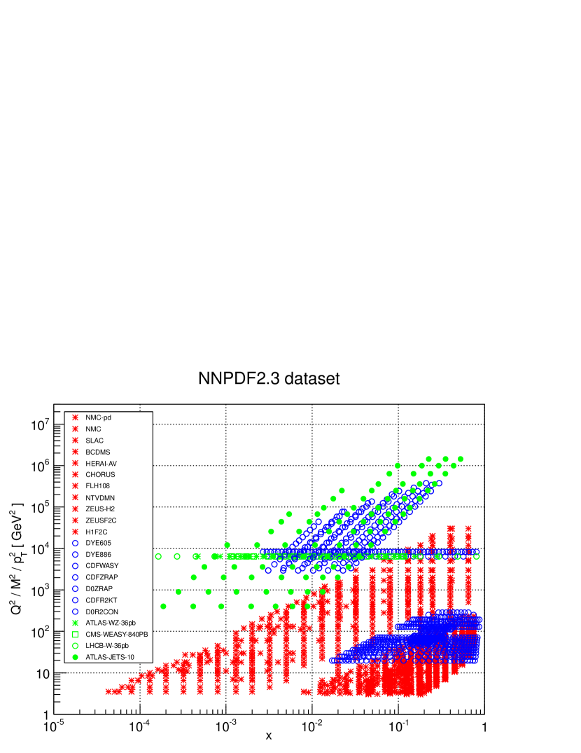
Figure 1: The kinematical coverage of the experimental data used in the NNPDF2.3 PDF determination, from Reference Ball:2012cx .

As discussed in Section 2, various alternative choices are possible in PDF determination both in terms of theory and methodology. The main choices which underlie the PDF sets we consider here are summarized in Table 3.

	MSTW08	CT10	NNPDF2.3	HERAPDF1.5	ABM11	JR09
No. of PDFs	7	6	7	5	6	5
Statistics	Hess.+DT	Hess.+DT	MC	Hess.+Model+Parm.	Hess.	Hess.+T
PDF parms.	20+8	25	259	14	24	12
Heavy quarks	VFN TR	VFN ACOT	VFN FONLL	VFN TR	FFN	FFN

Table 3: Main features of various NNLO PDF sets (see text for details).

All sets are now available at NLO and NNLO, and all but HERAPDF also have a LO version, though, as mentioned in Section 2.1.3, LO PDFs are often optimized for use with Monte Carlo event generators, and thus we will not discuss them further. The number of independently parametrized PDFs varies between seven (the three lighter quarks and antiquarks and the gluon), six (the total strangeness is independently parametrized, but not the strange and antistrange separately) or five (strangeness not fitted, and assumed to be a fixed fraction of the sea). The methodology for uncertainty representation and determination is Hessian, based on a parametrization of the form of Equation 22 for all groups except NNPDF, which uses a Monte Carlo representation based on a neural network parametrization (see Section 2.2). In order to determine confidence levels, CT and MSTW use dynamical tolerance, denoted in the table as “DT” (recall Section 2.2), JR use simple tolerance, denoted by “T”, HERAPDF uses $\Delta\chi^{2}=1$ but supplemented by an estimate of model and parametrization uncertainties, and ABM just use $\Delta\chi^{2}=1$. In each case the total number of free parameters at NNLO is as given in the table; the number of parameters at NLO is the same for all groups but CT10, which at NLO has 26 parameters, and HERAPDF1.5, which at NLO has only 10 parameters. MSTW08 uses 28 free parameters for the determination of the best fit, 8 of which are fixed when determining uncertainties. JR09 introduces the further “dynamical” assumption that PDFs are valence-like at a low scale $Q_{0}^{2}<1$ GeV². All groups but ABM and JR use variable-flavor number schemes, with heavy-quark masses included using one of the matching methods discussed in Section 2.1. The treatment of $\alpha_{S}$ will be discussed in more detail below.

3.1 Values and Uncertainties of Strong Coupling

An important issue which distinguishes PDF sets is the treatment of the strong coupling $\alpha_{S}(M_{Z}^{2})$. Because the value of $\alpha_{S}$ is strongly correlated with PDFs, one should always use in cross-section calculations PDFs which have been determined with the same value of $\alpha_{S}$ that is adopted for the calculation itself.

The value of $\alpha_{S}(M_{Z}^{2})$, and its uncertainty, can either be determined simultaneously with the PDFs or imposed as an external constraint. Furthermore, if the value of $\alpha_{S}$ is determined simultaneously with the PDFs, the quoted value of the PDF uncertainties may refer strictly to the PDF-only uncertainty as $\alpha_{S}$ is kept fixed at its best-fit value, or it may also include the uncertainty due to the variation of $\alpha_{S}$ itself.

The values of $\alpha_{S}(M_{Z}^{2})$ used by different NNLO PDF fitting groups are shown in Figure 2, where the larger symbols represent the default value used by each group, that is used for the determination of PDF uncertainties.

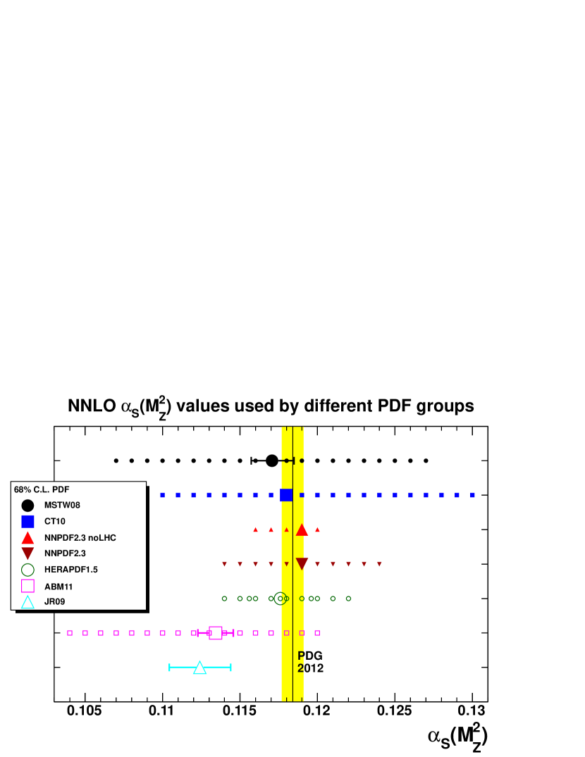
Figure 2: $\alpha_{S}(M_{Z}^{2})$ values for which NNLO PDFs are provided by various groups. The larger symbols denote the values used in subsequent plots.

For MSTW08, ABM11 and JR09, this value is determined from the fit with uncertainties shown by the horizontal error bars, while for CT it is chosen as a fixed value close to the PDG world average Beringer:1900zz , also shown in the plot. NNPDF do not have a default value and provide a full Monte Carlo replica set for each of the $\alpha_{S}$ values shown, though they have also presented an $\alpha_{S}$ determination Ball:2011us based on their previous NNPDF2.1 set, with results consistent with the PDG average. For NNPDF, which does not have a default value, we arbitrarily choose $\alpha_{S}(M_{Z}^{2})=0.119$ as default to be used in all plots, so that the MSTW08 and NNPDF $\alpha_{S}$ values bracket the CT10 value by providing a variation of $\Delta\alpha_{S}=0.001$ about it, for reasons to be discussed in Section 4.1.3 below.

The smaller symbols in Figure 2 indicate the PDF sets with alternative values of $\alpha_{S}(M_{Z}^{2})$ provided by each group. All groups provide only the best-fit PDF set for each of these values, except NNPDF which instead provide a full set for each value. The PDF uncertainties provided by MSTW and CT at the reference value of $\alpha_{S}$, and by NNPDF for all values of $\alpha_{S}$, do not include the $\alpha_{S}$ uncertainty, though MSTW also provide additional sets allowing combined PDF+$\alpha_{S}$ uncertainties Martin:2009bu . JR and ABM only provide combined PDF+$\alpha_{S}$ uncertainties.

3.2 Comparison of PDFs

A typical set of PDFs (MSTW08) at two different scales is shown in Figure 3.

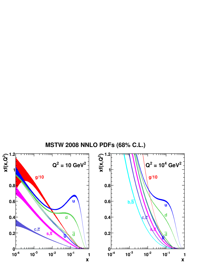
Figure 3: MSTW 2008 NNLO PDFs at $Q^{2}=10$ GeV² and $Q^{2}=10^{4}$ GeV², from Reference Martin:2009iq .

It is clear from Equation 2.1.1, however, that, in order to understand properties of hadronic cross sections and the impact of PDFs on them, it is more useful to consider the relevant parton–parton luminosities, defined as in Equation 4, rather than the PDFs themselves.

A detailed study would involve comparison of the luminosity for all parton combinations: for example, $\mathcal{L}_{u\bar{d}}$, relevant for $W^{+}$ production, and so forth. Here we only compare the $q\bar{q}$ luminosity summed over quark flavors, i.e.,

$$\sum_{q=u,d,s,c,b}\left(\mathcal{L}_{q\bar{q}}+\mathcal{L}_{\bar{q}q}\right),$$ (43)

where $\mathcal{L}_{ab}$ is defined in Equation 4.

(a)

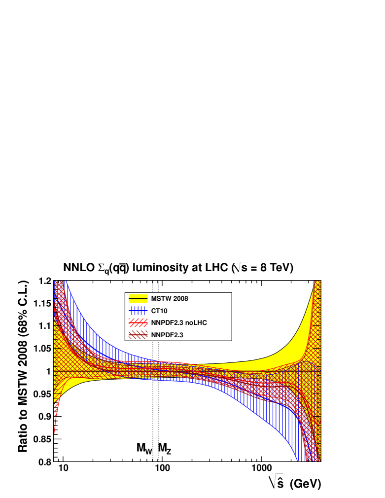
(b)

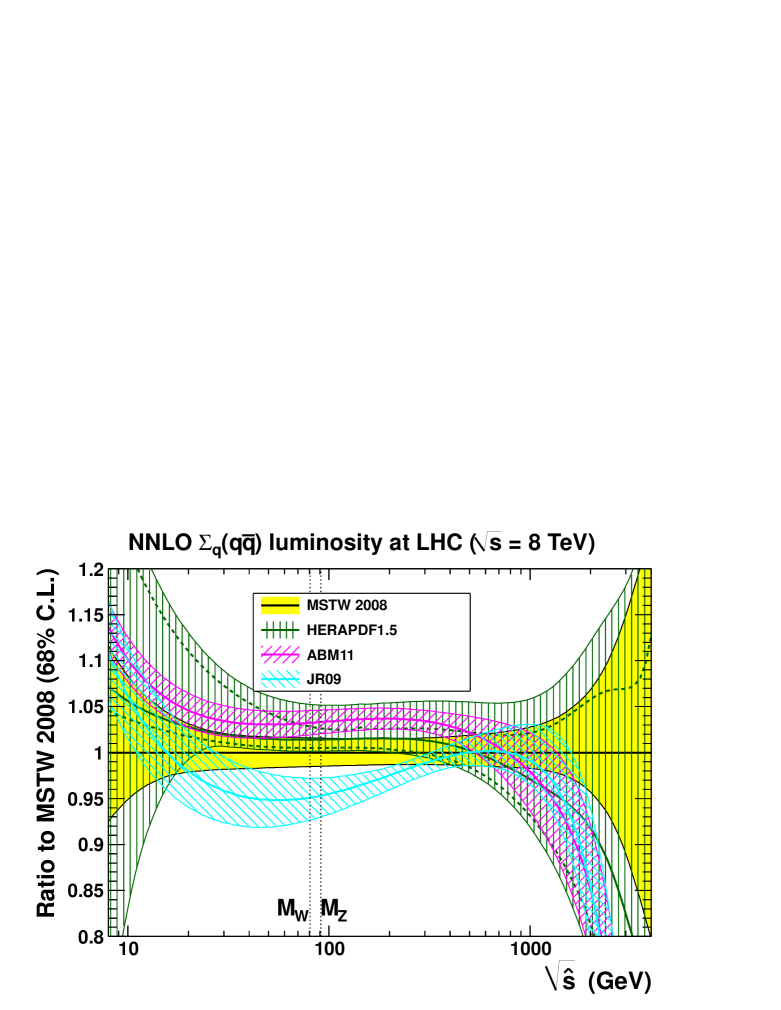
Figure 4: NNLO $q\bar{q}$ luminosity functions taken as the ratio to MSTW08. (a) MSTW08 vs. CT10 vs. NNPDF2.3noLHC vs. NNPDF2.3, then (b) MSTW08 vs. ABM11 vs. HERAPDF1.5 vs. JR09.

(a)

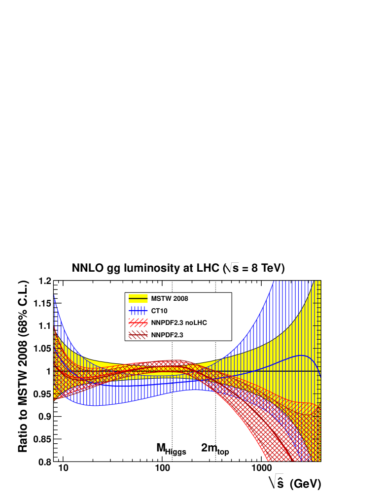
(b)

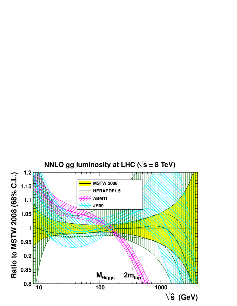
Figure 5: NNLO $gg$ luminosity functions taken as the ratio to MSTW08. (a) MSTW08 vs. CT10 vs. NNPDF2.3noLHC vs. NNPDF2.3, then (b) MSTW08 vs. ABM11 vs. HERAPDF1.5 vs. JR09.

In Figure 4 and Figure 5 we show, respectively, the NNLO $q\bar{q}$ and $gg$ luminosities, displayed as a ratio to the MSTW 2008 NNLO luminosities, for the LHC at $\sqrt{s}=8$ TeV, and in Figure 5 we show the corresponding NNLO $gg$ luminosities. We use the $\alpha_{S}$ values for each set shown in Figure 2. Note that all uncertainty bands are shown at 68% C.L., requiring the CT10 uncertainties (corresponding to a nominal 90% C.L.) to be divided by a factor of 1.64485. Similar plots, using a common value of $\alpha_{S}(M_{Z}^{2})=0.118$, can be found in Reference Ball:2012wy .

The relevant values of $\sqrt{\hat{s}}=M_{W,Z}$ are indicated for the $q\bar{q}$ luminosities, and the relevant values of $\sqrt{\hat{s}}=M_{H},2m_{t}$ (for $M_{H}=126$ GeV and $m_{t}=173.18$ GeV) are indicated for the $gg$ luminosities. There is fairly good agreement for the three global fits (MSTW08, CT10 and NNPDF2.3), but more variation for the other sets, which confirms that the dominant factor in determining the features of the PDFs is the choice of data set. There is little difference between the luminosities computed using NNPDF2.3 and NNPDF2.3noLHC, which shows that the impact of the LHC data is moderate. We will see in Section 4 that this is often but not always the case. The NLO trend between groups is similar to the NNLO trend, with the exception of HERAPDF at large $\hat{s}$ values, where the HERAPDF1.5 NLO set HERA:2010 has a much larger $q\bar{q}$ luminosity, and a much softer $gg$ luminosity, than other NLO PDF groups.

These luminosities are the basic input to LHC phenomenology, as we will discuss shortly. Current recommendations Botje:2011sn to use global fits for LHC searches and calibration, already mentioned in Section 1 and to be discussed in Section 4 below, were based on similar, more detailed comparisons of luminosities and PDFs made in 2010 Alekhin:2011sk . However, the situation is much improved now than in 2010, when only MSTW08 had a NNLO PDF set from a global fit, and differences at NLO between MSTW08, CTEQ6.6 and NNPDF2.0 were larger, due to, for example, the use of a less flexible gluon parametrization in CTEQ6.6 and the lack of inclusion of terms suppressed by powers of the charm-quark mass in NNPDF2.0.

A recent thorough analysis of PDFs and luminosities Ball:2012wy shows that the general features of NNLO global PDF sets, at a scale of order of $Q^{2}\sim M_{W}^{2}$, are the following, bearing in mind that experimental information is not available outside the region $10^{-4}\lesssim x\lesssim 0.4$ (see Figure 1). Up and down quark and antiquark distributions are known to an accuracy better than about $5\%$ in a wide range of $x$, roughly $10^{-4}\lesssim x\lesssim 0.3$ for the up distribution, $10^{-4}\lesssim x\lesssim 0.1$ for the down and the antiup distribution, $10^{-4}\lesssim x\lesssim 0.01$ for the antidown distribution, and there is good agreement between the three global sets. For smaller values of $x$, uncertainties gradually blow up, but there remains good agreement between sets as the behavior in this region is mostly driven by perturbative evolution, while, for larger values of $x$, uncertainties blow up and widely different behaviors are observed between sets: already for $x\sim 0.5$ uncertainties are likely to be bigger than $10\%$, and perhaps underestimated especially as $x$ grows. Strangeness is nominally known to about 10–15% accuracy in the region $0.003\lesssim x\lesssim 0.1$. However, it should be kept in mind that strangeness is largely determined by neutrino dimuon data (see Section 2.3.3), which are subject to various poorly controlled systematics, and also, one of the three global sets does not parametrize independently the $s$ and $\bar{s}$ distribution, while another only has a small number of parameters. Indeed, disagreement between different sets are up to the 30% level. The gluon distribution is known with an accuracy which is comparable or marginally worse than that of light quarks, i.e., $\sim 5\%$ at small $10^{-4}\lesssim x\lesssim 0.1$, but rapidly deteriorates at larger $x$, where it is only constrained by jet data. As already mentioned, here the agreement between global sets is not as good as one might hope, and discrepancies up to the level of 1.5–2 sigma between global fits are observed in the region $x\sim 0.02$, which is relevant for Higgs production.

Comparison of NLO and NNLO PDFs suggests that uncertainties related to higher-order corrections are smaller than $5\%$ in the region where PDFs are currently determined, meaning that the neglected theory uncertainties are likely to be smaller than the experimental PDF uncertainties at NNLO, whereas at NLO they might be comparable.

4 LHC PHENOMENOLOGY

The first LHC proton run was completed in December 2012, after a remarkable three years, with a center-of-mass energy of 7 TeV in 2010/2011 and 8 TeV in 2012. Data have been collected for a vast array of Standard Model processes. Many of these are already leading to new significant constraints on PDFs, with others holding the promise to do so in the very near future, and the knowledge of PDFs has played a significant rôle in the discovery of a Higgs-like particle Aad:2012gk ; Chatrchyan:2012gu . In this section, we confront LHC data with the predictions of various PDF sets for some key Standard Model total cross sections, specifically $W$, $Z$, Higgs boson and top-pair production, then we discuss methods for combining the predictions made using the PDF sets from different groups. We finally assess the current constraints on PDFs provided by LHC data and we examine the prospects for future improvements.

4.1 Predictions for LHC Cross Sections

A comprehensive study of the PDF dependence of key LHC cross sections has recently been made in Reference Ball:2012wy , following earlier work in References Alekhin:2011sk ; Watt:2011kp ; Watt:2012np . Here we will present some selected results from a continuation of the earlier study Alekhin:2011sk ; Watt:2011kp ; Watt:2012np , but now updated to account for the latest PDF sets and LHC data. The impact of LHC data will be discussed in more detail in Section 4.2, but we will already show here results with the two variants of NNPDF2.3, with and without LHC data, which will give us an indication of their current impact.

4.1.1 $W$ and $Z$ Production

The $W^{+}$, $W^{-}$ and $Z$ cross sections at the LHC differ from those at the Tevatron discussed in Section 2.3 because the LHC is a $pp$ rather than a $p\bar{p}$ collider. Hence, somewhat different combinations of the light quark and antiquark distributions are measured. To understand this, it is useful to consider the $W^{\pm}\equiv W^{+}+W^{-}$ to $Z^{0}$ cross-section ratio, and the $W^{+}$ to $W^{-}$ cross-section ratio. Assuming that very roughly $\bar{u}(x_{2})\approx\bar{d}(x_{2})$, and neglecting heavier quarks, one gets

$$\frac{\sigma_{W^{+}}+\sigma_{W^{-}}}{\sigma_{Z^{0}}}\sim\frac{u(x_{1})+d(x_{1})}{0.29\,u({x}_{1})+0.37\,d({x}_{1})},$$ (44)

$$\frac{\sigma_{W^{+}}}{\sigma_{W^{-}}}\sim\frac{u(x_{1})\,\bar{d}(x_{2})}{d(x_{1})\,\bar{u}(x_{2})}\sim\frac{u(x_{1})}{d(x_{1})},$$ (45)

where $x_{1}$ and $x_{2}$ are fixed when measuring a rapidity distribution, and we have assumed that $x_{1,2}$ are in a region where $q(x_{1})\bar{q}(x_{2})$ dominates over $\bar{q}(x_{1})q(x_{2})$. Equation 44 shows that the $W^{\pm}$ and $Z$ cross sections are very highly correlated (so that their ratio depends very little on the PDFs), while Equation 44 (to be compared to its counterpart at a $p\bar{p}$ collider, Equation 40) shows that the ratio of $W^{+}$/$W^{-}$ cross sections is a sensitive probe of the $u/d$ ratio.

We now consider explicitly predictions for $W$ and $Z$ production, where, for definiteness, we show results only for total cross sections. However, as mentioned, only rapidity distributions probe fixed leading-order parton kinematics. Furthermore, only around half of the total $W^{\pm}$ and $Z^{0}$ cross sections lie inside the acceptance of the ATLAS and CMS detectors, so that a theory calculation is needed to extrapolate the measurement over the whole phase space, introducing an additional uncertainty on the total cross sections. Therefore, data-to-theory comparisons for precision physics are best made at the level of the fiducial cross section (i.e., within the acceptance), which is possible at NNLO using the public fewz Gavin:2010az ; Gavin:2012sy and dynnlo Catani:2009sm codes, and indeed was done in the ATLAS publication Aad:2011dm .

(a)

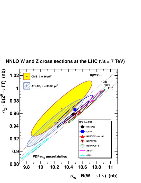
(b)

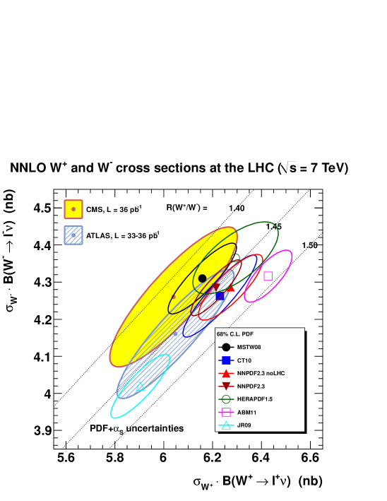
Figure 6: (a) $W^{\pm}$ vs. $Z^{0}$ and (b) $W^{+}$ vs. $W^{-}$ total cross sections at NNLO, compared to data from CMS CMS:2011aa and ATLAS Aad:2011dm . Lines (dotted) of constant ratio are also drawn for reference.

In Figure 6 we show $W^{\pm}\equiv W^{+}+W^{-}$ versus $Z^{0}$ and $W^{+}$ versus $W^{-}$ total cross sections. We also compare to the experimental measurements using the 2010 LHC data from ATLAS Aad:2011dm and CMS CMS:2011aa . The measured $Z^{0}$ cross sections have been corrected Watt:2011kp for the small $\gamma^{*}$ contribution and the finite invariant-mass range of the lepton pair (different for ATLAS and CMS) using a theory calculation at NNLO Anastasiou:2003ds . The ellipses are drawn to account for the correlations between the two cross sections, both for the experimental measurements and for the theoretical predictions, in such a way that the projection onto either axis gives the one-sigma uncertainty for the individual cross sections, so that the area of the two-dimensional ellipse corresponds to a confidence-level somewhat smaller than the conventional 68% cowan .

The spread in predictions using the different PDF sets is comparable to the (dominant) luminosity uncertainty of 4% (CMS) or 3.4% (ATLAS), with the JR09 prediction being a clear outlier. The correlation of $W^{\pm}$ and $Z$ cross sections is clearly visible from the plot. The impact of LHC data can be gauged by comparing the NNPDF2.3noLHC and NNPDF2.3 predictions: while for the $W^{\pm}$ and $Z$ cross sections there is essentially no difference, consistent with the stability of the $q\bar{q}$ luminosity of Figure 4, there is a clear reduction of uncertainty in the $W^{+}/W^{-}$ cross-section ratio, seen as a shrinking of the corresponding ellipse, which comes from an improved knowledge of the light flavor separation.

4.1.2 Higgs and Top-pair Production

Whereas the cross sections for production of $W$ and $Z$ bosons are sensitive to the quark distributions, we now turn to processes that are sensitive to the gluon distribution. The dominant production mechanism for both Standard Model Higgs bosons, or top-pairs, at the LHC is through gluon–gluon fusion. The $gg\to H$ process proceeds mainly through a top-quark loop, so both processes start at $\mathcal{O}(\alpha_{S}^{2})$ at LO and are directly sensitive to the value of $\alpha_{S}(M_{Z}^{2})$. Indeed, the CMS measurement of the $t\bar{t}$ cross section has even been used to extract $\alpha_{S}$ CMS:2012sxa . Moreover, the gluon PDF itself, being necessarily determined through strong-interaction processes, is the most sensitive to the value of $\alpha_{S}$. Therefore, for these observables we will present predictions for cross sections as a function of $\alpha_{S}(M_{Z}^{2})$.

(a)

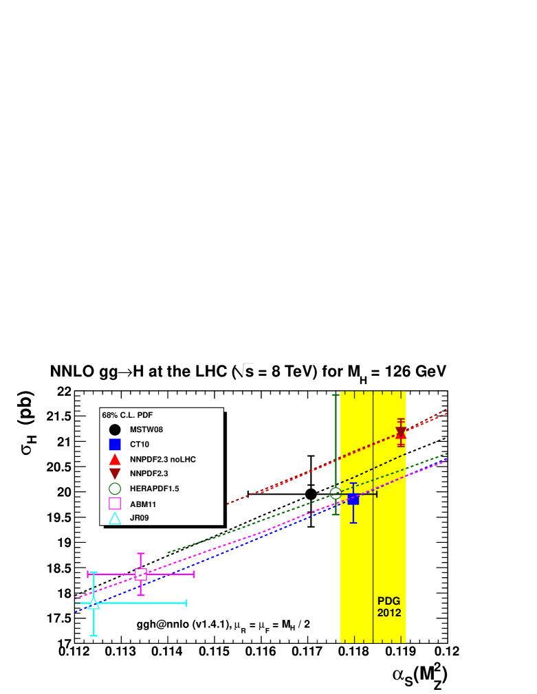
(b)

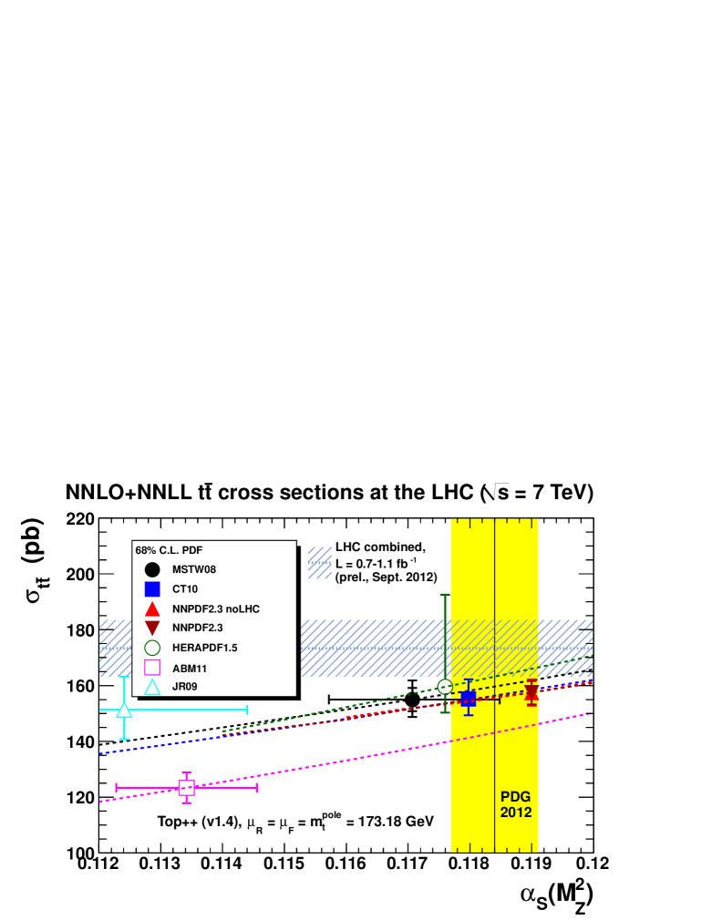
Figure 7: (a) NNLO $gg\to H$ total cross sections for $M_{H}=126$ GeV, and (b) NNLO_approx.+NNLL $t\bar{t}$ total cross sections for $m_{t}=173.18$ GeV, both plotted as a function of $\alpha_{S}(M_{Z}^{2})$.

The $gg\to H$ and $t\bar{t}$ cross sections are shown in Figure 7 for a Higgs mass $M_{H}=126$ GeV and a top-quark pole mass of $m_{t}=173.18$ GeV Aaltonen:2012ra , for the LHC at $8$ TeV and $7$ TeV, respectively, probing the gluon distribution at different $x\sim M_{H}/\sqrt{s}=0.02$ and $x\gtrsim 2m_{t}/\sqrt{s}=0.05$. For Higgs production we use the ggh@nnlo (version 1.4.1) code Harlander:2002wh with a scale choice of $\mu_{R}=\mu_{F}=M_{H}/2$, while for top-pair production we use the top++ (version 1.4) code Czakon:2012pz with a scale choice of $\mu_{R}=\mu_{F}=m_{t}$. Higgs production at NNLO, in the limit of a heavy top-quark mass, was originally calculated in References Harlander:2002wh ; Anastasiou:2002yz ; Ravindran:2003um . The top-pair calculations Czakon:2012pz include exact NNLO corrections for all quark-initiated processes (and $qg\to t\bar{t}$), with approximate NNLO for $gg\to t\bar{t}$, together with soft-gluon resummation to next-to-next-to-leading logarithmic accuracy. The markers in Figure 7 are centered on the $\alpha_{S}(M_{Z}^{2})$ values of Figure 2 and the corresponding predicted cross section of each PDF fitting group. The horizontal error bars span the $\alpha_{S}(M_{Z}^{2})$ uncertainty, while the vertical error bars span the PDF uncertainty, which (recall Section 3.1) for ABM11 and JR09 necessarily correspond to a combined PDF+$\alpha_{S}$ uncertainty. For MSTW08, the inner vertical error bars span the PDF only uncertainty and the outer vertical error bars span the PDF+$\alpha_{S}$ uncertainty.

The $\alpha_{S}$ dependence of results is shown from the dashed lines, which interpolate the cross-section predictions calculated using the sets with different $\alpha_{S}(M_{Z}^{2})$ values provided by each group. The vertical shaded band indicates the PDG world average value Beringer:1900zz of $\alpha_{S}(M_{Z}^{2})$, while the horizontal shaded band in Figure 7(b) indicates the preliminary combination of ATLAS and CMS $t\bar{t}$ cross-section measurements ATLAS:2012dpa ; CMS:2012dya . The scale dependence, obtained by varying $\mu_{R}$ and $\mu_{F}$ by factors of two, subject to the constraint $1/2\leq\mu_{R}/\mu_{F}\leq 2$, leads to a theoretical uncertainty of ${}^{+5.6}_{-4.9}\%$, while the top-mass dependence obtained by varying $m_{t}=173.18\pm 0.94$ GeV Aaltonen:2012ra leads to an uncertainty on the predicted cross section of $\pm 2.8\%$, where these percentage uncertainties were obtained using the central MSTW08 PDF set.

The strong dependence on the value of $\alpha_{S}$ is clearly seen. For the Higgs cross section it is interesting to observe (comparing also the $gg$ luminosity plot in Figure 5) that the value of $M_{H}\sim 126$ GeV with $\sqrt{s}=8$ TeV is especially unlucky, in that predictions obtained using global fits maximally disagree. Note that the NNPDF2.3 and NNPDF2.3noLHC in these plots are essentially identical: this shows that, unlike the $W$ data discussed above, the LHC jet data included in the NNPDF2.3 fit have a very moderate impact.

We see from Figure 7(b) that, even after accounting for all uncertainties, the ABM11 PDF set is strongly disfavored by both the LHC top-pair cross section and the world average value of $\alpha_{S}(M_{Z}^{2})$. The ABM11 prediction of $\sigma_{t\bar{t}}=123.3\pm 5.5(\mathrm{PDF+}\alpha_{S})^{+6.2}_{-5.6}(\textrm{scales})^{+3.6}_{-3.5}(m_{t})~{}\textrm{pb}$ is almost 30% below the measured cross section of $\sigma_{t\bar{t}}=173.3\pm 10.1~{}\textrm{pb}$, whereas adding all experimental and theoretical uncertainties in quadrature still gives a total uncertainty of less than 8%. We note also from Figure 7 that the HERAPDF1.5 NNLO predictions have a very large model uncertainty in the upwards direction, due to varying the minimum $Q^{2}$ cut from the default value of $Q^{2}_{\rm min}=3.5~{}{\rm GeV}^{2}$ to a slightly higher value of $Q^{2}_{\rm min}=5~{}{\rm GeV}^{2}$. This sensitivity is not observed in global fits, where the Tevatron jet data stabilize the fit and so lessen sensitivity to the fine details of the treatment of the DIS data Thorne:2011kq ; Watt:2012np .

4.1.3 Combination of Results from Different PDF Groups

Whereas it is often advisable to check experimental results against predictions obtained using the widest available set of PDFs, there are situations where a unique reliable prediction is needed. Typical examples are searches for new physics, or acceptance calculations, where one does not want to inflate uncertainties unnaturally, but also does not want to mistake an underestimated systematic effect for a new physics effect, as has sometimes happened in the past.

This suggests that use of PDF sets based on significantly smaller data sets is not advisable, as these necessarily have larger uncertainties (and indeed sometimes have appeared as outliers, as seen above). As mentioned in Section 1, the PDF4LHC group recommended therefore Botje:2011sn the use of the CTEQ, MSTW and NNPDF PDFs based on global fits for these purposes at the LHC. This recommendation was adopted by the Higgs working group Dittmaier:2011ti , and used for Higgs searches and discovery Aad:2012gk ; Chatrchyan:2012gu .

The problem however arises of the best way to combine results from different groups. The PDF4LHC group originally recommended taking an envelope of various predictions, i.e., taking as a 68% C.L. the range between the top of the highest one-sigma bands, and the bottom of the lowest, with the midpoint as a central value. This choice is simple to implement, but it has no clear-cut statistical meaning. A better option is to take a statistical combination as originally proposed in Reference Forte:2010dt and discussed in Section 2.2.3. Results obtained either way are shown in Figure 8, where in order to construct the statistical combination 100 Monte Carlo replicas were generated for MSTW08 and CT10 from the original Hessian sets using the method described in Reference Watt:2012tq ; see Equation 28. It is clear that the two methods actually produce fairly similar results, though the envelope method is somewhat more conservative, especially when there is some disagreement between predictions.

(a)                                                                  (b)

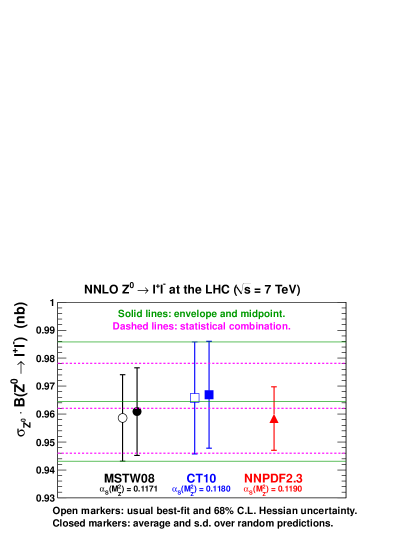
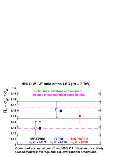
(c)                                                                  (d)

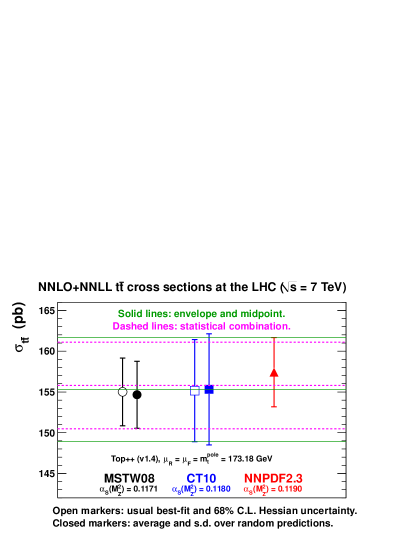
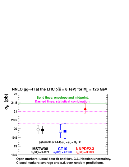
Figure 8: NNLO (a) $Z^{0}$, (b) $W^{+}/W^{-}$, (c) $t\bar{t}$ and (d) $gg\to H$ cross sections from MSTW08, CT10 and NNPDF2.3, combined either by taking the envelope of the three predictions, or from the statistical combination of 100 random predictions from each group.

A separate issue is how to treat the $\alpha_{S}$ uncertainty. The original PDF4LHC prescription recommended a very conservative approach in which one takes the envelope of three PDF+$\alpha_{S}$ uncertainties, each centered at a different central value of $\alpha_{S}$: this was motivated by the feeling that the PDG $\alpha_{S}(M_{Z}^{2})$ uncertainty of $\Delta\alpha_{S}=0.0007$ might be somewhat underestimated. The uncertainties shown in Figure 8 are PDF-only uncertainties for a fixed $\alpha_{S}$ value. However, results for the three PDF sets are obtained using the three different central values shown in Figure 2, so the combination implicitly includes an additional uncertainty arising from the different $\alpha_{S}$ values of $\alpha_{S}(M_{Z}^{2})=0.118\pm 0.001$, without going into the complication of computing explicit PDF+$\alpha_{S}$ uncertainties on each separate prediction.

4.2 PDF Constraints From the LHC

The LHC data have already started bringing in new information on PDFs. This is expected to be even more the case in the coming years as more processes will be studied thoroughly. Indeed, as mentioned in Section 2.2.1, full information on the correlations between the systematic uncertainties is necessary if data are to be used for PDF determination. This is at present only available for a handful of measurements (in particular those used in NNPDF2.3, see Figure 1), but this situation is rapidly changing. In fact, it is likely that in the next one or two decades most information on PDFs, which will be crucial for new physics searches at the LHC, will be coming from the LHC itself. The only possible exception is if the proposed Large Hadron–electron Collider (LHeC) AbelleiraFernandez:2012cc were to be built. This would lead to a very substantial increase in knowledge of high-energy deep-inelastic scattering which, using separate information on charged- and neutral-current processes, together with charm tagging, would allow complete flavor separation from DIS alone (as discussed in Section 2.3), while the large lever arm in $Q^{2}$ would allow an accurate determination of the gluon from scaling violations. More accurate results on flavor separation could only be obtained at a neutrino factory Mangano:2001mj .

4.2.1 Light Flavors

The strongest constraint on light flavor PDF at the LHC comes from the combination of rapidity distributions for the production of various gauge bosons: as repeatedly mentioned, a rapidity distribution fixes entirely the leading-order parton kinematics. If full information on the correlation between different processes is retained, a global fit including all of them effectively uses the information provided by all the various cross-section ratios that are sensitive to different PDF combinations, such as Equations 44 and 45, or, equivalently the asymmetry

$$\frac{\sigma_{W^{+}}-\sigma_{W^{-}}}{\sigma_{W^{+}}+\sigma_{W^{-}}}\sim\frac{u_{v}(x_{1})-d_{v}(x_{1})}{u(x_{1})+d(x_{1})}.$$ (46)

It is important to observe that many sources of systematics are common (such as for instance the normalization) to these cross sections and cancel in the ratio: hence the availability of full correlations leads to potentially much more precise results. Given that the LHC energy is being increased in stages, it is also possible to form ratios or double ratios between measurements at different energies which further increase the potential for precision Mangano:2012mh .

The most discriminating data on $W$ production so far are the CMS asymmetry data Chatrchyan:2012xt , included in the NNPDF2.3 fit, and which are mostly responsible for the sizable reduction in uncertainty seen in Figure 6(b) when comparing the NNPDF2.3 and NNPDF2.3noLHC fits. These measurements have in particular shown that the asymmetry is underestimated by the MSTW08 fit, implying that $u_{v}-d_{v}$ is too small at $x\sim M_{W}/\sqrt{s}\sim 0.01$.

(a)

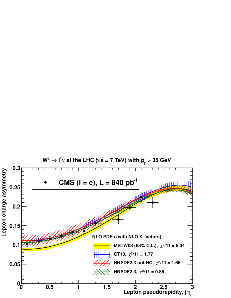
(b)

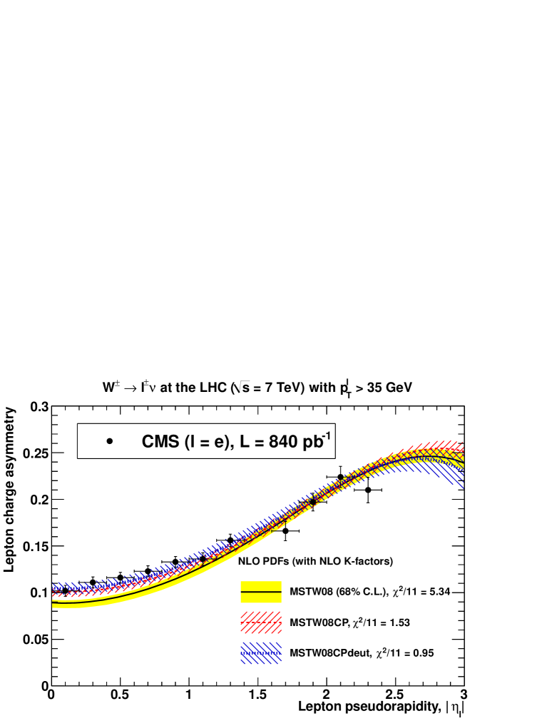
Figure 9: Description of CMS electron asymmetry Chatrchyan:2012xt using (a) various NLO PDF sets, and (b) improved variants of the MSTW08 analysis Martin:2012da .

In Figure 9 we show the CMS data from Reference Chatrchyan:2012xt with $p_{T}^{\ell}>35$ GeV. It is apparent that inclusion of these data in the NNPDF2.3 analysis resulted in a more than three-fold reduction in the NLO PDF uncertainty on the asymmetry at central pseudorapidity. They prompted a reexamination of the PDF parametrization (and also deuteron corrections) used in the MSTW08 fit, where an extended Chebyshev parametrization form and more flexible deuteron corrections were found to automatically improve the description of the CMS electron asymmetry data Martin:2012da ; see Figure 9(b). (Figure 9 shows only NLO PDF sets since the main studies of Reference Martin:2012da were done at this order). This is an example of how present and future LHC data may help in resolving discrepancies which are still present between PDF sets.

In addition to $W$ and $Z$ production, measurements of Drell–Yan processes ($Z/\gamma^{*}\to\ell\ell$ or $W\to\ell\nu$) away from the resonance peaks at $M_{\ell\ell}=M_{Z}$ or $M_{\ell\nu}=M_{W}$ in either direction can provide complementary constraints on different PDF combinations and $x$ values.

4.2.2 Gluon

The NNPDF2.3 analysis also includes inclusive jet data from ATLAS Aad:2011fc . These could in principle result in a reduction of uncertainties on the gluon distribution at the $x$ values in the intermediate region shown in Figure 1, though in practice their impact is very moderate, as seen from the luminosity plot in Figure 5 and the Higgs and top production cross sections in Figure 7. This situation is likely to change in the future, as jet data become more abundant and precise. For example, the recent CMS jet data Chatrchyan:2012bz are expected to place more stringent constraints on the gluon distribution than the available ATLAS data Aad:2011fc .

As is clear from Figure 7, data for top-pair production, especially differential distributions Chatrchyan:2012qka , will provide stringent constraints on the gluon. The process is only known at NLO at the differential level, but at the inclusive level the full NNLO result is just around the corner Czakon:2012pz . Eventually, once all aspects of the observed Higgs-like boson are understood, even Higgs production itself (which at least in the Standard Model is known up to NNLO) could be perhaps the most sensitive probe of the gluon distribution.

Other LHC data may be used to constrain the gluon distribution. A particularly clean probe might come from gauge-boson $p_{T}$ distributions, because the final-state $W$ or $Z$ can acquire a $p_{T}$ dependence only if at least one parton is radiated. The values of $p_{T}$ accessible at the LHC are large enough that it should be possible to obtain significant constraints even by imposing a cut in order to avoid the low $p_{T}$ region where QCD resummation is mandatory and non-perturbative effects might become relevant. The impact on PDFs of these data, some of which are already available Aad:2011gj ; Chatrchyan:2011wt , has not been studied yet. However, as with the closely related observable of $W,Z$+jet production, only a NLO ($\mathcal{O}(\alpha_{S}^{2})$) calculation is available.

Another classic process which may be used to constrain the gluon distribution is prompt photon production, and the related photon+jet production process, to which gluons contribute at leading order. Inclusion of present-day LHC prompt photon data would only lead to a moderate reduction of order of $\sim 20\%$ of the gluon uncertainty d'Enterria:2012yj at medium-small $x\sim 0.02$, with photon+jet data having an even milder impact Carminati:2012mm , but future data are likely to be much more constraining. Here, the main bottleneck is that theoretical predictions are only available up to NLO, and higher order corrections are likely to be large. Diphoton production is known up to NNLO Catani:2011qz , but it is less constraining in that the gluon contribution only starts at NLO.

A potential option to get a handle on the gluon is the study of $W$ polarization Chatrchyan:2011ig ; ATLAS:2012au ; Stirling:2012zt , which is similar to the $W$ $p_{T}$ distribution discussed above, but subject to small QCD corrections Bern:2011ie .

4.2.3 Strangeness and Heavy Quarks

As already discussed in Section 2.3.3, $W$ production also provides a handle on strangeness, and in fact Tevatron $W$ production data were found Ball:2010de to have a significant impact on the $s-\bar{s}$ distribution. It has been argued Aad:2012sb that a fit only to inclusive $W^{\pm}$ and $Z$ differential cross sections Aad:2011dm , combined with inclusive DIS data from HERA, can significantly constrain the strange content of the proton, finding apparently no strange suppression, contrary to previous determinations from CCFR/NuTeV dimuon cross sections ($\nu N\to\mu\mu X$). However, these conclusions are weakened in a similar NNPDF study using a more flexible parametrization form Ball:2012cx , or alternatively by incorporating a suitable tolerance Watt:2012tq , and it seems that present-day LHC $W$ production data only have a very minor impact on strangeness, but this is again likely to change in the near future.

A much more direct handle on strangeness at the LHC comes from $W$ production with an associated charm-tagged jet, where the dominant partonic subprocesses are $\bar{s}\,g\to W^{+}\,\bar{c}$ and $s\,g\to W^{-}\,c$. A first preliminary measurement has been made by CMS CMS:2011lqa of the cross-section ratios $R_{c}\equiv\sigma(W+c)/\sigma(W+{\rm jets})$, probing the strange content of the proton relative to other light-quark flavors, and $R_{c}^{\pm}\equiv\sigma(W^{+}+\bar{c})/\sigma(W^{-}+c)$, potentially probing the strange asymmetry. With more precise measurements to come, including differential distributions, the $W$+charm process should enable powerful constraints to be made on the $s$ and $\bar{s}$ distributions Stirling:2012vh . The main limitation here is that only NLO results are available for this process.

Similarly, $Z$ production in association with a tagged charm jet will provide significant constraints on the charm distribution Stirling:2012vh , and likewise, $Z$ with a $b$ jet on the $b$ distribution.

5 THE FUTURE OF PDF DETERMINATION

Parton distributions have become increasingly relevant with the advent of the LHC. After the landmark discovery of a Higgs-like boson in July 2012 Aad:2012gk ; Chatrchyan:2012gu , focus now shifts to characterizing the properties of this new particle, as well as increasingly difficult searches for indications of other new physics. As a consequence, demand will grow to reduce the unavoidable uncertainties associated with the PDFs in calculations of both signal and background. On the one hand, it will be necessary to bring under complete control the uncertainties in the region of electroweak symmetry breaking, i.e., the region of $x$ and $Q^{2}$ which is probed by Higgs production. In this region, as mentioned in Section 3.2, uncertainties are in principle small, but in practice for some PDFs such as the gluon and even more the strange, discrepancies between different sets at the one or two sigma level are seen and not fully understood. On the other hand, searches for new physics will involve heavy final states, and thus, because of Equation 3, they will involve knowledge of PDFs in the large $x\gtrsim 0.5$ region where they are currently very poorly known. To achieve these goals, it will be necessary to construct PDFs which satisfy a number of criteria, that not so long ago Forte:2010dt characterized an ideal PDF determination, but in the LHC era have become necessary requirements, namely, in decreasing order of importance:

1. The range and precision of data sets must be as wide as possible, cover currently unexplored kinematic regions, and include new LHC processes, such as those discussed in Section 4.2, which will gradually remove current discrepancies between PDF determinations.

2. The parametrization should be sufficiently general and demonstrably unbiased, either by using a sufficiently large number of parameters, or by careful a posteriori checks of parametrization independence.

3. The experimental uncertainties should be understood and carefully propagated, and in particular the statistical meaning of the procedures that are being adopted to determine the PDF uncertainties should be understood: specifically, the choice of tolerance, and the determination of the optimal fit when using a very flexible parametrization.

4. Computations should be performed at the highest available perturbative order, and in particular, at the order which is subsequently to be used in the computation of partonic cross sections. This is currently NNLO, but the need for the inclusion of various kinds of all-orders resummation is becoming increasingly important. For example, computations which include Sudakov resummation are already being used in the computation of the Higgs production cross section deFlorian:2012yg , and for consistency resummed computations should also be used in PDF determination Corcella:2005us : this becomes especially important in the large $x\gtrsim 0.5$ region that will be probed in searches for new physics. Also, the inclusion of resummation effects will be increasingly important in the construction of PDFs to be used in fixed-order calculations matched to parton showers in Monte Carlo event generators. Finally, PDFs including electroweak corrections will have to be constructed Martin:2004dh .

5. The treatment of heavy quarks will have to include mass-suppressed terms in the coefficient functions, while also resumming logarithmically enhanced terms via the evolution equations. Such a treatment, like the schemes discussed in Section 2.1.3, is a minimum requirement: this is currently standard for DIS, but applications to hadronic observables are so far limited. Also, the dependence of results on the choice of value for the heavy-quark masses will have to be studied more systematically, possibly using the perturbatively more stable $\overline{\rm MS}$ mass definition Alekhin:2010sv , with PDF sets made available for several values of the heavy-quark masses.

6. The strong coupling $\alpha_{S}$, in addition to being determined simultaneously with PDFs, should also be decoupled from the PDF determination, with PDF sets available for a range of fixed $\alpha_{S}$ values, and full PDF uncertainty determination for each value of $\alpha_{S}$.

7. Estimate of theoretical uncertainties will have to be performed together with PDF sets, and such uncertainties will have to be provided each time they become comparable with other sources of PDF uncertainty. This is presently an almost unexplored territory.

We predict that, as the needs of precision physics at the LHC develop, more and more of these features will become accepted standards.

- (1) ATLAS Collaboration, G. Aad et al., Observation of a new particle in the search for the Standard Model Higgs boson with the ATLAS detector at the LHC, Phys.Lett. B716 (2012) 1–29, [arXiv:1207.7214].
- (2) CMS Collaboration, S. Chatrchyan et al., Observation of a new boson at a mass of 125 GeV with the CMS experiment at the LHC, Phys.Lett. B716 (2012) 30–61, [arXiv:1207.7235].
- (3) R. McElhaney and S. F. Tuan, Some consequences of a modified Kuti Weisskopf quark parton model, Phys. Rev. D8 (1973) 2267–2272.
- (4) T. Kawaguchi and H. Nakkagawa, “Analysis of Scaling Violation in Terms of Theories with Anomalous Dimensions.” KUNS 380, 1976.
- (5) A. De Rujula, H. Georgi, and H. D. Politzer, Demythification of Electroproduction, Local Duality and Precocious Scaling, Ann. Phys. 103 (1977) 315.
- (6) P. W. Johnson and W.-k. Tung, Comparison of Asymptotically Free Theories with High-Energy Deep Inelastic Scattering Data, Nucl. Phys. B121 (1977) 270.
- (7) M. Glück and E. Reya, Operator Mixing and Scaling Deviations in Asymptotically Free Field Theories, Phys. Rev. D14 (1976) 3034–3044.
- (8) I. Hinchliffe and C. H. Llewellyn Smith, Detailed Treatment of Scaling Violations in Asymptotically Free Gauge Theories, Nucl. Phys. B128 (1977) 93.
- (9) A. J. Buras and K. J. F. Gaemers, Simple Parametrizations of Parton Distributions with Dependence Given by Asymptotic Freedom, Nucl. Phys. B132 (1978) 249.
- (10) M. Glück, E. Hoffmann, and E. Reya, Scaling Violations and the Gluon Distribution of the Nucleon, Zeit. Phys. C13 (1982) 119.
- (11) D. W. Duke and J. F. Owens, Dependent Parametrizations of Parton Distribution Functions, Phys. Rev. D30 (1984) 49–54.
- (12) E. Eichten, I. Hinchliffe, K. D. Lane, and C. Quigg, Super Collider Physics, Rev. Mod. Phys. 56 (1984) 579–707.
- (13) A. Devoto, D. W. Duke, J. F. Owens, and R. G. Roberts, Direct Analysis of Scaling Violations in Large Deep Inelastic Neutrino and Muon Scattering, Phys. Rev. D27 (1983) 508–522.
- (14) A. D. Martin, R. G. Roberts, and W. J. Stirling, Structure Function Analysis and , Jet, , Production: Pinning Down the Gluon, Phys. Rev. D37 (1988) 1161.
- (15) M. Diemoz, F. Ferroni, E. Longo, and G. Martinelli, Parton Densities from Deep Inelastic Scattering to Hadronic Processes at Super Collider Energies, Z. Phys. C39 (1988) 21.
- (16) M. Glück, E. Reya, and A. Vogt, Radiatively generated parton distributions for high-energy collisions, Z. Phys. C48 (1990) 471–482.
- (17) J. G. Morfin and W.-K. Tung, Parton distributions from a global QCD analysis of deep inelastic scattering and lepton pair production, Z. Phys. C52 (1991) 13–30.
- (18) CTEQ Collaboration, H. L. Lai et al., Global QCD analysis of parton structure of the nucleon: CTEQ5 parton distributions, Eur. Phys. J. C12 (2000) 375–392, [hep-ph/9903282].
- (19) A. D. Martin, R. G. Roberts, W. J. Stirling, and R. S. Thorne, MRST2001: Partons and from precise deep inelastic scattering and Tevatron jet data, Eur. Phys. J. C23 (2002) 73–87, [hep-ph/0110215].
- (20) S. Alekhin, Extraction of parton distributions and from DIS data within the Bayesian treatment of systematic errors, Eur. Phys. J. C10 (1999) 395–403, [hep-ph/9611213].
- (21) V. Barone, C. Pascaud, and F. Zomer, A new global analysis of deep inelastic scattering data, Eur. Phys. J. C12 (2000) 243–262, [hep-ph/9907512].
- (22) M. Botje, A QCD analysis of HERA and fixed target structure function data, Eur. Phys. J. C14 (2000) 285–297, [hep-ph/9912439].
- (23) W. T. Giele and S. Keller, Implications of hadron collider observables on parton distribution function uncertainties, Phys.Rev. D58 (1998) 094023, [hep-ph/9803393].
- (24) W. T. Giele, S. A. Keller, and D. A. Kosower, Parton distribution function uncertainties, hep-ph/0104052.
- (25) J. Pumplin, D. R. Stump, J. Huston, H. L. Lai, P. M. Nadolsky, et al., New generation of parton distributions with uncertainties from global QCD analysis, JHEP 0207 (2002) 012, [hep-ph/0201195].
- (26) A. D. Martin, R. G. Roberts, W. J. Stirling, and R. S. Thorne, Uncertainties of predictions from parton distributions. I: Experimental errors, Eur. Phys. J. C28 (2003) 455–473, [hep-ph/0211080].
- (27) A. D. Martin, W. J. Stirling, R. S. Thorne, and G. Watt, Parton distributions for the LHC, Eur.Phys.J. C63 (2009) 189–285, [arXiv:0901.0002].
- (28) H.-L. Lai, M. Guzzi, J. Huston, Z. Li, P. M. Nadolsky, et al., New parton distributions for collider physics, Phys.Rev. D82 (2010) 074024, [arXiv:1007.2241].
- (29) S. Forte, L. Garrido, J. I. Latorre, and A. Piccione, Neural network parametrization of deep inelastic structure functions, JHEP 0205 (2002) 062, [hep-ph/0204232].
- (30) NNPDF Collaboration, R. D. Ball et al., A Determination of parton distributions with faithful uncertainty estimation, Nucl.Phys. B809 (2009) 1–63, [arXiv:0808.1231].
- (31) NNPDF Collaboration, R. D. Ball, L. Del Debbio, S. Forte, A. Guffanti, J. I. Latorre, et al., A first unbiased global NLO determination of parton distributions and their uncertainties, Nucl.Phys. B838 (2010) 136–206, [arXiv:1002.4407].
- (32) M. Glück, P. Jimenez-Delgado, and E. Reya, Dynamical parton distributions of the nucleon and very small- physics, Eur.Phys.J. C53 (2008) 355–366, [arXiv:0709.0614].
- (33) P. Jimenez-Delgado and E. Reya, Dynamical NNLO parton distributions, Phys.Rev. D79 (2009) 074023, [arXiv:0810.4274].
- (34) S. Alekhin, J. Blümlein, S. Klein, and S. Moch, The 3, 4, and 5-flavor NNLO Parton from Deep-Inelastic-Scattering Data and at Hadron Colliders, Phys.Rev. D81 (2010) 014032, [arXiv:0908.2766].
- (35) S. Alekhin, J. Blümlein, and S. Moch, Parton Distribution Functions and Benchmark Cross Sections at NNLO, Phys.Rev. D86 (2012) 054009, [arXiv:1202.2281].
- (36) S. Alekhin, Parton distributions from deep-inelastic scattering data, Phys. Rev. D68 (2003) 014002, [hep-ph/0211096].
- (37) S. Alekhin, Parton distribution functions from the precise NNLO QCD fit, JETP Lett. 82 (2005) 628–631, [hep-ph/0508248].
- (38) H1 and ZEUS Collaboration, F. D. Aaron et al., Combined Measurement and QCD Analysis of the Inclusive Scattering Cross Sections at HERA, JHEP 1001 (2010) 109, [arXiv:0911.0884].
- (39) H1 and ZEUS Collaboration, F. D. Aaron et al., “PDF fits including HERA-II high data (HERAPDF1.5).” H1prelim-10-141, ZEUS-prel-10-017.
- (40) H1 and ZEUS Collaboration, F. D. Aaron et al., “HERAPDF1.5 NNLO.” H1prelim-11-042, ZEUS-prel-11-002.
- (41) S. Alekhin, J. Blümlein, P. Jimenez-Delgado, S. Moch, and E. Reya, NNLO Benchmarks for Gauge and Higgs Boson Production at TeV Hadron Colliders, Phys.Lett. B697 (2011) 127–135, [arXiv:1011.6259].
- (42) S. Alekhin, S. Alioli, R. D. Ball, V. Bertone, J. Blümlein, et al., The PDF4LHC Working Group Interim Report, arXiv:1101.0536.
- (43) G. Watt, Parton distribution function dependence of benchmark Standard Model total cross sections at the 7 TeV LHC, JHEP 1109 (2011) 069, [arXiv:1106.5788].
- (44) G. Watt, MSTW PDFs and impact of PDFs on cross sections at Tevatron and LHC, Nucl.Phys.Proc.Suppl. 222-224 (2012) 61–80, [arXiv:1201.1295].
- (45) R. D. Ball, S. Carrazza, L. Del Debbio, S. Forte, J. Gao, et al., Parton Distribution Benchmarking with LHC Data, arXiv:1211.5142.
- (46) M. Botje, J. Butterworth, A. Cooper-Sarkar, A. de Roeck, J. Feltesse, et al., The PDF4LHC Working Group Interim Recommendations, arXiv:1101.0538.
- (47) LHC Higgs Cross Section Working Group Collaboration, S. Dittmaier et al., Handbook of LHC Higgs Cross Sections: 1. Inclusive Observables, arXiv:1101.0593.
- (48) S. Forte, Parton distributions at the dawn of the LHC, Acta Phys.Polon. B41 (2010) 2859–2920, [arXiv:1011.5247].
- (49) A. De Roeck and R. S. Thorne, Structure Functions, Prog.Part.Nucl.Phys. 66 (2011) 727–781, [arXiv:1103.0555].
- (50) E. Perez and E. Rizvi, The Quark and Gluon Structure of the Proton, arXiv:1208.1178.
- (51) J. F. Owens and W.-K. Tung, Parton distribution functions of hadrons, Ann.Rev.Nucl.Part.Sci. 42 (1992) 291–332.
- (52) R. K. Ellis, W. J. Stirling, and B. R. Webber, QCD and collider physics. Cambridge Univ. Press, Cambridge, UK, 1996.
- (53) J. Collins, Foundations of perturbative QCD. Cambridge Univ. Press, Cambridge, UK, 2011.
- (54) M. R. Whalley, D. Bourilkov, and R. C. Group, The Les Houches accord PDFs (lhapdf) and lhaglue, hep-ph/0508110.
- (55) A. Vogt, Efficient evolution of unpolarized and polarized parton distributions with qcd-pegasus, Comput. Phys. Commun. 170 (2005) 65–92, [hep-ph/0408244].
- (56) G. P. Salam and J. Rojo, A Higher Order Perturbative Parton Evolution Toolkit (hoppet), Comput. Phys. Commun. 180 (2009) 120–156, [arXiv:0804.3755].
- (57) M. Botje, qcdnum: Fast QCD Evolution and Convolution, Comput.Phys.Commun. 182 (2011) 490–532, [arXiv:1005.1481].
- (58) W. Giele et al., The QCD/SM working group: Summary report, hep-ph/0204316.
- (59) M. Dittmar et al., Parton distributions: Summary report, hep-ph/0511119.
- (60) S. Moch, J. A. M. Vermaseren, and A. Vogt, The Three loop splitting functions in QCD: The Nonsinglet case, Nucl.Phys. B688 (2004) 101–134, [hep-ph/0403192].
- (61) A. Vogt, S. Moch, and J. A. M. Vermaseren, The Three-loop splitting functions in QCD: The Singlet case, Nucl.Phys. B691 (2004) 129–181, [hep-ph/0404111].
- (62) C. Anastasiou, L. J. Dixon, K. Melnikov, and F. Petriello, Dilepton rapidity distribution in the Drell-Yan process at NNLO in QCD, Phys.Rev.Lett. 91 (2003) 182002, [hep-ph/0306192].
- (63) J. A. M. Vermaseren, A. Vogt, and S. Moch, The Third-order QCD corrections to deep-inelastic scattering by photon exchange, Nucl.Phys. B724 (2005) 3–182, [hep-ph/0504242].
- (64) S. Moch, J. A. M. Vermaseren, and A. Vogt, Third-order QCD corrections to the charged-current structure function , Nucl.Phys. B813 (2009) 220–258, [arXiv:0812.4168].
- (65) J. M. Campbell, J. W. Huston, and W. J. Stirling, Hard Interactions of Quarks and Gluons: A Primer for LHC Physics, Rept.Prog.Phys. 70 (2007) 89, [hep-ph/0611148].
- (66) A. Buckley, J. Butterworth, S. Gieseke, D. Grellscheid, S. Hoche, et al., General-purpose event generators for LHC physics, Phys.Rept. 504 (2011) 145–233, [arXiv:1101.2599].
- (67) A. Sherstnev and R. S. Thorne, Parton Distributions for LO Generators, Eur.Phys.J. C55 (2008) 553–575, [arXiv:0711.2473].
- (68) H.-L. Lai, J. Huston, S. Mrenna, P. Nadolsky, D. Stump, et al., Parton Distributions for Event Generators, JHEP 1004 (2010) 035, [arXiv:0910.4183].
- (69) T. Kasemets and T. Sjostrand, A Comparison of new MC-adapted Parton Densities, Eur.Phys.J. C69 (2010) 19–29, [arXiv:1007.0897].
- (70) T. Appelquist and J. Carazzone, Infrared Singularities and Massive Fields, Phys.Rev. D11 (1975) 2856.
- (71) J. C. Collins, F. Wilczek, and A. Zee, Low-Energy Manifestations of Heavy Particles: Application to the Neutral Current, Phys.Rev. D18 (1978) 242.
- (72) M. Aivazis, J. C. Collins, F. I. Olness, and W.-K. Tung, Leptoproduction of heavy quarks. 2. A Unified QCD formulation of charged and neutral current processes from fixed target to collider energies, Phys.Rev. D50 (1994) 3102–3118, [hep-ph/9312319].
- (73) J. C. Collins, Hard scattering factorization with heavy quarks: A General treatment, Phys.Rev. D58 (1998) 094002, [hep-ph/9806259].
- (74) M. Guzzi, P. M. Nadolsky, H.-L. Lai, and C.-P. Yuan, General-Mass Treatment for Deep Inelastic Scattering at Two-Loop Accuracy, Phys.Rev. D86 (2012) 053005, [arXiv:1108.5112].
- (75) R. S. Thorne and R. G. Roberts, An Ordered analysis of heavy flavor production in deep inelastic scattering, Phys.Rev. D57 (1998) 6871–6898, [hep-ph/9709442].
- (76) R. S. Thorne and R. G. Roberts, A Practical procedure for evolving heavy flavor structure functions, Phys.Lett. B421 (1998) 303–311, [hep-ph/9711223].
- (77) R. S. Thorne, A Variable-flavor number scheme for NNLO, Phys.Rev. D73 (2006) 054019, [hep-ph/0601245].
- (78) M. Cacciari, M. Greco, and P. Nason, The spectrum in heavy flavor hadroproduction, JHEP 9805 (1998) 007, [hep-ph/9803400].
- (79) S. Forte, E. Laenen, P. Nason, and J. Rojo, Heavy quarks in deep-inelastic scattering, Nucl.Phys. B834 (2010) 116–162, [arXiv:1001.2312].
- (80) J. Rojo et al., “Chapter 22 in: J. R. Andersen and others., The SM and NLO multileg working group: Summary report.” arXiv:1003.1241, 2010.
- (81) M. Buza, Y. Matiounine, J. Smith, and W. L. van Neerven, Charm electroproduction viewed in the variable-flavour number scheme versus fixed-order perturbation theory, Eur. Phys. J. C1 (1998) 301–320, [hep-ph/9612398].
- (82) M. Roth and S. Weinzierl, QED corrections to the evolution of parton distributions, Phys.Lett. B590 (2004) 190–198, [hep-ph/0403200].
- (83) A. D. Martin, R. G. Roberts, W. J. Stirling, and R. S. Thorne, Parton distributions incorporating QED contributions, Eur.Phys.J. C39 (2005) 155–161, [hep-ph/0411040].
- (84) G. Cowan, Statistical data analysis. Oxford Univ. Press, Oxford, UK, 1998.
- (85) D. Stump, J. Pumplin, R. Brock, D. Casey, J. Huston, et al., Uncertainties of predictions from parton distribution functions. 1. The Lagrange multiplier method, Phys.Rev. D65 (2001) 014012, [hep-ph/0101051].
- (86) G. D’Agostini, On the use of the covariance matrix to fit correlated data, Nucl.Instrum.Meth. A346 (1994) 306–311.
- (87) NNPDF Collaboration, R. D. Ball et al., Fitting Parton Distribution Data with Multiplicative Normalization Uncertainties, JHEP 1005 (2010) 075, [arXiv:0912.2276].
- (88) S. Brodsky, P. Hoyer, C. Peterson, and N. Sakai, The Intrinsic Charm of the Proton, Phys.Lett. B93 (1980) 451–455.
- (89) J. Pumplin, H. Lai, and W. Tung, The Charm Parton Content of the Nucleon, Phys.Rev. D75 (2007) 054029, [hep-ph/0701220].
- (90) R. G. Roberts, The structure of the proton. Cambridge Univ. Press, Cambridge, UK, 1990.
- (91) A. Glazov, S. Moch, and V. Radescu, Parton Distribution Uncertainties using Smoothness Prior, Phys.Lett. B695 (2011) 238–241, [arXiv:1009.6170].
- (92) J. Pumplin, Parametrization dependence and in parton distribution fitting, Phys.Rev. D82 (2010) 114020, [arXiv:0909.5176].
- (93) A. D. Martin, A. J. T. M. Mathijssen, W. J. Stirling, R. S. Thorne, B. J. A. Watt, et al., Extended Parameterisations for MSTW PDFs and their effect on Lepton Charge Asymmetry from W Decays, arXiv:1211.1215.
- (94) J. C. Collins and J. Pumplin, Tests of goodness of fit to multiple data sets, hep-ph/0105207.
- (95) NNPDF Collaboration, L. Del Debbio, S. Forte, J. I. Latorre, A. Piccione, and J. Rojo, Neural network determination of parton distributions: The Nonsinglet case, JHEP 0703 (2007) 039, [hep-ph/0701127].
- (96) NNPDF Collaboration, R. D. Ball, V. Bertone, F. Cerutti, L. Del Debbio, S. Forte, et al., Impact of Heavy Quark Masses on Parton Distributions and LHC Phenomenology, Nucl.Phys. B849 (2011) 296–363, [arXiv:1101.1300].
- (97) NNPDF Collaboration, R. D. Ball et al., Unbiased global determination of parton distributions and their uncertainties at NNLO and at LO, Nucl.Phys. B855 (2012) 153–221, [arXiv:1107.2652].
- (98) G. Watt and R. S. Thorne, Study of Monte Carlo approach to experimental uncertainty propagation with MSTW 2008 PDFs, JHEP 1208 (2012) 052, [arXiv:1205.4024].
- (99) NNPDF Collaboration, R. D. Ball et al., Reweighting NNPDFs: the lepton asymmetry, Nucl.Phys. B849 (2011) 112–143, [arXiv:1012.0836].
- (100) NNPDF Collaboration, R. D. Ball, V. Bertone, F. Cerutti, L. Del Debbio, S. Forte, et al., Reweighting and Unweighting of Parton Distributions and the LHC lepton asymmetry data, Nucl.Phys. B855 (2012) 608–638, [arXiv:1108.1758].
- (101) J. Pumplin, Experimental consistency in parton distribution fitting, Phys.Rev. D81 (2010) 074010, [arXiv:0909.0268].
- (102) NNPDF Collaboration, R. D. Ball et al., Parton Distributions: Determining Probabilities in a Space of Functions, arXiv:1110.1863.
- (103) R. S. Thorne, Effect of changes of variable flavor number scheme on parton distribution functions and predicted cross sections, Phys.Rev. D86 (2012) 074017, [arXiv:1201.6180].
- (104) A. D. Martin, R. G. Roberts, W. J. Stirling, and R. S. Thorne, Uncertainties of predictions from parton distributions. II: Theoretical errors, Eur. Phys. J. C35 (2004) 325–348, [hep-ph/0308087].
- (105) NNPDF Collaboration, R. D. Ball et al., Precision determination of electroweak parameters and the strange content of the proton from neutrino deep-inelastic scattering, Nucl.Phys. B823 (2009) 195–233, [arXiv:0906.1958].
- (106) M. L. Mangano, S. I. Alekhin, M. Anselmino, R. D. Ball, M. Boglione, et al., Physics at the front end of a neutrino factory: A Quantitative appraisal, hep-ph/0105155.
- (107) S. D. Ellis and W. J. Stirling, Constraints on isospin breaking in the light quark sea from the Drell-Yan process, Phys.Lett. B256 (1991) 258–264.
- (108) E. L. Berger, F. Halzen, C. Kim, and S. Willenbrock, WEAK BOSON PRODUCTION AT TEVATRON ENERGIES, Phys.Rev. D40 (1989) 83.
- (109) A. D. Martin, R. G. Roberts, and W. J. Stirling, Improved Parton Distributions and , Production at Colliders, Mod.Phys.Lett. A4 (1989) 1135.
- (110) P. Nadolsky, J. Gao, M. Guzzi, J. Huston, H.-L. Lai, et al., Progress in CTEQ-TEA PDF Analysis, arXiv:1206.3321.
- (111) NNPDF Collaboration, R. D. Ball, V. Bertone, S. Carrazza, C. S. Deans, L. Del Debbio, et al., Parton distributions with LHC data, Nucl.Phys. B867 (2013) 244–289, [arXiv:1207.1303].
- (112) Particle Data Group Collaboration, J. Beringer et al., Review of Particle Physics (RPP), Phys.Rev. D86 (2012) 010001.
- (113) NNPDF Collaboration, R. D. Ball, V. Bertone, L. Del Debbio, S. Forte, A. Guffanti, et al., Precision NNLO determination of using an unbiased global parton set, Phys.Lett. B707 (2012) 66–71, [arXiv:1110.2483].
- (114) A. D. Martin, W. J. Stirling, R. S. Thorne, and G. Watt, Uncertainties on in global PDF analyses and implications for predicted hadronic cross sections, Eur.Phys.J. C64 (2009) 653–680, [arXiv:0905.3531].
- (115) R. Gavin, Y. Li, F. Petriello, and S. Quackenbush, fewz 2.0: A code for hadronic production at next-to-next-to-leading order, Comput.Phys.Commun. 182 (2011) 2388–2403, [arXiv:1011.3540].
- (116) R. Gavin, Y. Li, F. Petriello, and S. Quackenbush, Physics at the LHC with fewz 2.1, arXiv:1201.5896.
- (117) S. Catani, L. Cieri, G. Ferrera, D. de Florian, and M. Grazzini, Vector boson production at hadron colliders: A Fully exclusive QCD calculation at NNLO, Phys.Rev.Lett. 103 (2009) 082001, [arXiv:0903.2120].
- (118) ATLAS Collaboration, G. Aad et al., Measurement of the inclusive and cross sections in the electron and muon decay channels in collisions at TeV with the ATLAS detector, Phys.Rev. D85 (2012) 072004, [arXiv:1109.5141].
- (119) CMS Collaboration, S. Chatrchyan et al., Measurement of the Inclusive and Production Cross Sections in Collisions at TeV, JHEP 1110 (2011) 132, [arXiv:1107.4789].
- (120) C. Anastasiou, L. J. Dixon, K. Melnikov, and F. Petriello, High precision QCD at hadron colliders: Electroweak gauge boson rapidity distributions at NNLO, Phys.Rev. D69 (2004) 094008, [hep-ph/0312266].
- (121) CMS Collaboration, S. Chatrchyan et al., First Determination of the Strong Coupling Constant from the Cross Section, 2012. CMS-PAS-TOP-12-022.
- (122) CDF and DØ Collaboration, T. Aaltonen et al., Combination of the top-quark mass measurements from the Tevatron collider, Phys.Rev. D86 (2012) 092003, [arXiv:1207.1069].
- (123) R. V. Harlander and W. B. Kilgore, Next-to-next-to-leading order Higgs production at hadron colliders, Phys.Rev.Lett. 88 (2002) 201801, [hep-ph/0201206].
- (124) M. Czakon and A. Mitov, NNLO corrections to top pair production at hadron colliders: the quark-gluon reaction, JHEP 1301 (2013) 080, [arXiv:1210.6832].
- (125) C. Anastasiou and K. Melnikov, Higgs boson production at hadron colliders in NNLO QCD, Nucl.Phys. B646 (2002) 220–256, [hep-ph/0207004].
- (126) V. Ravindran, J. Smith, and W. L. van Neerven, NNLO corrections to the total cross-section for Higgs boson production in hadron hadron collisions, Nucl.Phys. B665 (2003) 325–366, [hep-ph/0302135].
- (127) ATLAS Collaboration, G. Aad et al., Combination of ATLAS and CMS top-quark pair cross section measurements using up to 1.1 fb-1 of data at 7 TeV, 2012. ATLAS-CONF-2012-134, ATLAS-COM-CONF-2012-166.
- (128) CMS Collaboration, S. Chatrchyan et al., Combination of ATLAS and CMS top-quark pair cross section measurements using proton-proton collisions at TeV, 2012. CMS-PAS-TOP-12-003.
- (129) R. S. Thorne and G. Watt, PDF dependence of Higgs cross sections at the Tevatron and LHC: Response to recent criticism, JHEP 1108 (2011) 100, [arXiv:1106.5789].
- (130) LHeC Study Group Collaboration, J. L. Abelleira Fernandez et al., A Large Hadron Electron Collider at CERN: Report on the Physics and Design Concepts for Machine and Detector, J.Phys. G39 (2012) 075001, [arXiv:1206.2913].
- (131) M. L. Mangano and J. Rojo, Cross Section Ratios between different CM energies at the LHC: opportunities for precision measurements and BSM sensitivity, JHEP 1208 (2012) 010, [arXiv:1206.3557].
- (132) CMS Collaboration, S. Chatrchyan et al., Measurement of the electron charge asymmetry in inclusive production in collisions at TeV, Phys.Rev.Lett. 109 (2012) 111806, [arXiv:1206.2598].
- (133) ATLAS Collaboration, G. Aad et al., Measurement of inclusive jet and dijet production in collisions at TeV using the ATLAS detector, Phys.Rev. D86 (2012) 014022, [arXiv:1112.6297].
- (134) CMS Collaboration, S. Chatrchyan et al., Measurements of differential jet cross sections in proton-proton collisions at TeV with the CMS detector, arXiv:1212.6660.
- (135) CMS Collaboration, S. Chatrchyan et al., Measurement of differential top-quark pair production cross sections in colisions at TeV, arXiv:1211.2220.
- (136) ATLAS Collaboration, G. Aad et al., Measurement of the transverse momentum distribution of bosons in proton-proton collisions at TeV with the ATLAS detector, Phys.Lett. B705 (2011) 415–434, [arXiv:1107.2381].
- (137) CMS Collaboration, S. Chatrchyan et al., Measurement of the Rapidity and Transverse Momentum Distributions of Bosons in Collisions at TeV, Phys.Rev. D85 (2012) 032002, [arXiv:1110.4973].
- (138) D. d’Enterria and J. Rojo, Quantitative constraints on the gluon distribution function in the proton from collider isolated-photon data, Nucl.Phys. B860 (2012) 311–338, [arXiv:1202.1762].
- (139) L. Carminati, C. Costa, D. d’Enterria, I. Koletsou, G. Marchiori, et al., Sensitivity of the LHC isolated-gamma+jet data to the parton distribution functions of the proton, arXiv:1212.5511.
- (140) S. Catani, L. Cieri, D. de Florian, G. Ferrera, and M. Grazzini, Diphoton production at hadron colliders: a fully-differential QCD calculation at NNLO, Phys.Rev.Lett. 108 (2012) 072001, [arXiv:1110.2375].
- (141) CMS Collaboration, S. Chatrchyan et al., Measurement of the Polarization of Bosons with Large Transverse Momenta in +Jets Events at the LHC, Phys.Rev.Lett. 107 (2011) 021802, [arXiv:1104.3829].
- (142) ATLAS Collaboration, G. Aad et al., Measurement of the polarisation of bosons produced with large transverse momentum in collisions at TeV with the ATLAS experiment, Eur.Phys.J. C72 (2012) 2001, [arXiv:1203.2165].
- (143) W. J. Stirling and E. Vryonidou, Electroweak gauge boson polarisation at the LHC, JHEP 1207 (2012) 124, [arXiv:1204.6427].
- (144) Z. Bern, G. Diana, L. Dixon, F. Febres Cordero, D. Forde, et al., Left-Handed W Bosons at the LHC, Phys.Rev. D84 (2011) 034008, [arXiv:1103.5445].
- (145) ATLAS Collaboration, G. Aad et al., Determination of the strange quark density of the proton from ATLAS measurements of the and cross sections, Phys.Rev.Lett. 109 (2012) 012001, [arXiv:1203.4051].
- (146) CMS Collaboration, S. Chatrchyan et al., Study of associated charm production in final states at TeV, 2011. CMS-PAS-EWK-11-013.
- (147) W. J. Stirling and E. Vryonidou, Charm production in association with an electroweak gauge boson at the LHC, Phys.Rev.Lett. 109 (2012) 082002, [arXiv:1203.6781].
- (148) D. de Florian and M. Grazzini, Higgs production at the LHC: updated cross sections at TeV, Phys.Lett. B718 (2012) 117–120, [arXiv:1206.4133].
- (149) G. Corcella and L. Magnea, Soft-gluon resummation effects on parton distributions, Phys.Rev. D72 (2005) 074017, [hep-ph/0506278].
- (150) S. Alekhin and S. Moch, Heavy-quark deep-inelastic scattering with a running mass, Phys.Lett. B699 (2011) 345–353, [arXiv:1011.5790].