Measuring the Casimir force gradient from graphene on a $\mbox{SiO}_{2}$ substrate

Abstract

The gradient of the Casimir force between a Si-SiO₂-graphene substrate and an Au-coated sphere is measured by means of a dynamic atomic force microscope operated in the frequency shift technique. It is shown that the presence of graphene leads to up to 9% increase in the force gradient at the shortest separation considered. This is in qualitative agreement with the predictions of Lifshitz theory using the dielectric permittivities of Si and SiO₂ and the Dirac model of graphene.

I Introduction

In the last few years graphene has attracted considerable attention as a material of much promise for nanotechnology due to its unique mechanical, electrical and optical properties.1 ; 2 Noting that at short separations between test bodies the fluctuation-induced dispersion interactions, such as the van der Waals and Casimir forces, become dominant,2a it is important to investigate them in the presence of a graphene sheet. In this connection much theoretical work has been done on the calculation of dispersion forces between two graphene sheets,3 ; 3a ; 4 ; 5 ; 6 ; 7a a graphene sheet and a metallic, dielectric or semiconductor plate,4 ; 5 ; 6 ; 7 ; 8 ; 9 ; 10 ; 11 ; 12 a graphene sheet and an atom or a molecule13 ; 14 ; 15 ; 16 etc. The calculations were performed using phenomenological density-functional methods,17 ; 18 ; 19 ; 20 second order perturbation theory,21 and the Lifshitz theory with some specific form for the reflection coefficients of electromagnetic oscillations on graphene.3 ; 5 ; 8 ; 9 However, in spite of the impressive progress in measurements of the Casimir force in configurations with metallic, dielectric and semiconductor test bodies (see reviews in Refs. 22 ; 23 ; 24 ; 25 and more recent experiments 26 ; 27 ; 28 ), there is yet no previous measurement of dispersion forces acting on graphene.

In the present paper we report measurements of the gradient of the Casimir force acting between a graphene sheet deposited on a SiO₂ film covering a Si plate and an Au-coated sphere. Our measurements are performed by means of dynamic atomic force microscope (AFM) operated in the frequency-shift technique described in detail in Refs. 27 ; 28 . We demonstrate significant increase in the gradient of the Casimir force in comparison with that between a Si plate covered with a SiO₂ film and an Au-coated sphere, i.e., in the absence of graphene sheet. At short separations this increase is up to a factor 4-5 larger than the total experimental error in the measurement of the force gradient determined at a 67% confidence level. We also compare the experimental results with an approximate theory where the gradients of the Casimir force between a Si-SiO₂ system and Au-coated sphere and between a graphene described by the Dirac model and the same sphere are computed independently of one another using the Lifshitz theory and then are added. Some excess of the theoretical force gradient over the experimental one is attributed to the screening of the Si-SiO₂ surface by a graphene sheet.

The paper is organized as follows. In Sec. II we briefly describe the detection system, the measurement scheem and the sample preparation. Section III contains the measurement results and their comparison with theory. Section IV contains our conclusions.

II Experimental setup

The detection system used in our measurements consists of an AFM cantilever with attached hollow glass microsphere coated with Au, piezoelectric actuators, fiber interferometers, light source, and phase locked loop (PLL). The thickness of the Au coating and the radius of the coated sphere were measured to be 280 nm and $54.10\pm 0.09\,\mu$m using an AFM and a scanning electron microscope, respectively. A turbo-pump, oil-free dry scroll mechanical-pump and ion-pump were used to achieve high vacuum down to $10^{-9}\,$Torr (see Refs. 27 ; 28 for detail of the setup).

In the dynamic measurement scheme the total force $F_{\rm tot}(a)=F_{\rm el}(a)+F(a)$ acting on the sphere [where $F_{\rm el}(a)$ and $F(a)$ are the electric and Casimir force, respectively, and $a$ is the separation distance between the sphere and graphene] modifies the resonant natural frequency of the oscillator. The change in the frequency $\Delta\omega=\omega_{r}-\omega_{0}$, where $\omega_{r}$ and $\omega_{0}$ are the resonance frequencies in the presence and in the absence of external force $F_{\rm tot}(a)$, respectively, was recorded by the PLL. This was done at every 0.14 nm while the plate was moved towards the grounded sphere starting at the maximum separation. This was repeated with one of 10 different voltages $V_{i}$ in the range from –38.5 to 58.4 mV for the first graphene sample and from –5.2 to 97.4 mV for the second graphene sample applied to the graphene sheet while the sphere remained grounded. The application of voltages and respective measurements were repeated for two times resulting in 20 sets of $\Delta\omega$ as a function of separation for each graphene sample.

Large area graphene used in our experiment was obtained through a two-step Chemical Vapor Deposition (CVD) process described.29 In this process $25\,\mu$m thick polycrystalline copper foil (99.8% purity) was cleaned by diluted HCl solution followed by deionized water rinse. Then the copper foil was placed into $\sim 5\,\mbox{cm}\times 3\,$cm copper bag which had undergone the same clean process as above. The copper bag was loaded into a ceramic tube furnace for the CVD process. First the copper bag was annealed at $1000^{\circ}$C under continuous Ar/H₂ (69 sccm/10 sccm) flow. Graphene was grown on the copper foil by introducing methane/hydrogen gas of 1.3 sccm/4 sccm for one hour and 35 sccm/4 sccm for another hour. Then the furnace was cooled down to room temperature under a continuous flow of Ar/H₂ (69 sccm/10 sccm). Finally, the grown graphene was transferred from the copper foil to 300 nm SiO₂ layer on a B-doped Si layer of $500\,\mu$m thickness on the bottom by using poly-metil methacrylate (PMMA) as the graphene support layer and ammonium persulfate solution as the copper etchant. We have examined the quality of the graphene layer through Raman spectroscopy 30a ; 30b and quantum Hall effect measurements,30c ; 30d which show single layer graphene characteristics. Measurements of 2D-mobility for a large area graphene onto SiO₂ substrates performed in our laboratory demonstrate mobility above $3000\,\mbox{cm}^{2}/\mbox{Vs}$. A roughly estimate for the concentration of impurities would be $1.2\times 10^{10}\,\mbox{cm}^{-2}$, if we consider that each impurity adsorbs one electron.

The gradients of the total and Casimir forces were found from the measured frequency shifts using electrostatic calibration. To perform this calibration of the setup, we used the expression for the electric force in sphere-plate geometry 23

$$F_{\rm el}(a)=X(a,R)(V_{i}-V_{0})^{2}.$$ (1)

Here $X(a,R)$ is a known function and $V_{0}$ is the residual potential difference between a sphere surface and a graphene sheet which is nonzero even when both surfaces are grounded. In the linear regime which is realized in our setup 27 the gradient of the Casimir force is given by

$$F^{\prime}(a)\equiv\frac{\partial F(a)}{\partial a}=-\frac{1}{C}\Delta\omega-\frac{\partial X(a,R)}{\partial a}(V_{i}-V_{0})^{2},$$ (2)

where $C=\omega_{0}/(2k)$ and $k$ is the spring constant of the cantilever. Note that the absolute separations between the zero level of the roughness on the sphere and graphene are found from $a=z_{\rm piezo}+z_{0}$, where $z_{\rm piezo}$ is the plate movement due to the piezoelectric actuator and $z_{0}$ is the closest approach between the Au sphere and graphene (in dynamic experiments the latter is much larger than the separation on contact of the two surfaces).

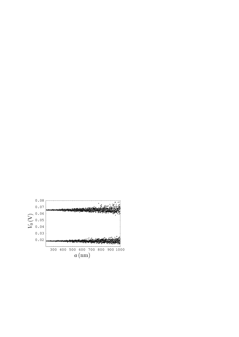
Figure 1: The residual potential difference between an Au-coated sphere and the first (lower dots) and second (upper dots) graphene sheets on a Si-SiO₂ substrate as a function of separation. The mean values of $V_{0}$ are shown by the gray lines.

From the position of a maximum in the parabolic dependence of $\Delta\omega$ on $V_{i}$ in Eq. (2), one can determine $V_{0}$ with the help of a $\chi^{2}$-fitting procedure. From the curvature of the parabola with the help of the same fit it is possible to determine $z_{0}$ and $C$. This was done at different separations for the two graphene samples used in our experiment. In Fig. 1 we present the values of $V_{0}$ as a function of separation determined from the fit for the first and second graphene samples (the lower and upper sets of dots, respectively). The obtained values were corrected for mechanical drift of the frequency-shift signal, as discussed in Ref. 27 . As can be seen from Fig. 1, the resulting $V_{0}$ do not depend on separation. To check this observation, we have performed the best fit of $V_{0}$ to the straight lines shown in Fig. 1 leaving their slopes as free parameters. It was found that the slopes are $-4.96\times 10^{-6}\,$mV/nm and $6.2\times 10^{-4}\,$mV/nm for the first and second samples, respectively, i.e., the independence of $V_{0}$ on $a$ was confirmed to a high accuracy. This finally leads to the mean values $V_{0}=18.4\pm 0.9\,$mV and $V_{0}=65.7\pm 0.9\,$mV for the first and second samples, respectively, where errors are determined at a 67% confidence level. Note that different graphene sheets may lead to different $V_{0}$ due to occasional impurities. The possible impurities could be organic, H₂, O₂, N₂ and H₂O. All these may become dopants of graphene and change its work function. Next the quantities $z_{0}$ and $C$ were determined from the fit at different separations and found to be separation-independent. For the first and second samples the mean values are equal to $z_{0}=222.5\pm 0.4\,$nm, $C=58.7\pm 0.17\,$kHz m/N and $z_{0}=222.2\pm 0.4\,$nm, $C=58.9\pm 0.17\,$kHz m/N, respectively. From the measured resonant frequency we have confirmed that the obtained value of $C$ results in the spring constant $k$ consistent with the estimated value provided by the cantilever fabricator.

III Measurement results and comparison with theory

For each graphene sample the gradients of the Casimir force $F^{\prime}(a)$ as a function of $a$ were obtained from the measured $\Delta\omega$ in two ways: by applying 10 different voltages $V_{i}$ with subsequent subtraction of the electric forces (2 repetitions) and by applying the compensating voltage $V_{i}=V_{0}$ (22 repetitions). In these cases 20 and 22 force-distance relations were obtained, the mean force gradients were computed and their total experimental errors were determined at a 67% confidence level as a combination of random and systematic errors (see Ref. 27 for details). In Fig. 2(a,b) the mean gradients of the Casimir force and their errors measured for the first sample with applied compensating voltage are shown as crosses with a step of 1 nm. Table  1 presents the values of mean $F^{\prime}(a)$ at several separations measured in the two different ways for the first (columns a, b) and second (columns c, d) samples. As can be seen in Table 1, the measurement results for the two graphene samples obtained in two different ways are in very good mutual agreement.

Now we compare the experimental results with theoretical predictions. At the moment there is no theory allowing rigorous calculation of the Casimir force between a graphene deposited on a Si-SiO₂ substrate and an Au sphere. The problem is that Si and SiO₂ layers are described by their dielectric permittivities and the reflection properties of graphene in the Dirac model are described by the polarization tensor. This does not allow direct application of the Lifshitz theory for layered structures 23 ; 30 . Because of this, here we restrict ourselves to the approximate approach, where the contributions of Si-SiO₂ substrate and graphene sheet to the Casimir interaction with an Au sphere are computed separately using the Lifshitz theory and are then added together. In the framework of the proximity force approximation (PFA), the Lifshitz formula for the gradient of the Casimir force between an Au sphere and any planar structure takes the form

$$F^{\prime}(a)=2k_{B}TR\sum_{l=0}^{\infty}{\vphantom{\sum}}^{\prime}\!\!\int_{0}^{\infty}\!\!\!\!q_{l}k_{\bot}dk_{\bot}\sum_{\alpha}\frac{r_{\alpha}^{(1)}r_{\alpha}^{(2)}}{e^{2q_{l}a}-r_{\alpha}^{(1)}r_{\alpha}^{(2)}}.$$ (3)

Here $k_{B}$ is the Boltzmann constant, $T=300\,$K is the laboratory temperature, $k_{\bot}$ is the projection of the wave vector on a planar structure, $q_{l}^{2}=k_{\bot}^{2}+\xi_{l}^{2}/c^{2}$, and $\xi_{l}=2\pi k_{B}Tl/\hbar$ with $l=0,\,1,\,2,\,\ldots$ are the Matsubara frequencies. The prime near the summation sign multiplies the term with $l=0$ by 1/2, and $\alpha={\rm TM,TE}$ denotes the transverse magnetic and transverse electric polarizations of the electromagnetic field. Note that an error arising from the application of PFA was recently found 31 ; 32 ; 33 using the exact theory for the sphere-plate geometry and was shown to be less than $a/R$, i.e., of about 0.5% in our experiment.

The quantity $r_{\alpha}^{(1)}=r_{\alpha}^{(1)}(i\xi_{l},k_{\bot})$ in Eq. (3) is the standard Fresnel reflection coefficient for an Au surface calculated at the imaginary frequencies (an Au layer can be considered as a semispace). It is expressed in terms of the dielectric permittivity $\varepsilon^{\,\rm Au}(i\xi_{l})$ using the tabulated optical data for Au 34 extrapolated to zero frequency either by the Drude or by the plasma models.22 ; 23

Unlike the case when a graphene layer is present, the Casimir interaction of the Si-SiO₂ substrate with an Au sphere is described by the well tested fundamental Lifshitz theory. Here the quantity $r_{\alpha}^{(2)}=r_{\alpha}^{(2)}(i\xi_{l},k_{\bot})$ has the meaning of the reflection coefficient on the two-layer (Si-SiO₂) structure 23 ; 30 ; 35 where Si can be considered as a semispace. It is expressed in terms of $\varepsilon^{\,\rm Si}(i\xi_{l})$ and $\varepsilon^{\,{\rm SiO}_{2}}(i\xi_{l})$. In our computations we used $\varepsilon^{\,\rm Si}(i\xi_{l})$ obtained 36 from the optical data 37 for Si extrapolated to zero frequency either by the Drude or by the plasma models (Si plate used has the resistivity between 0.001 and $0.005\,\Omega\,$cm which corresponds to a plasma frequency between $5\times 10^{14}$ and $11\times 10^{14}\,$rad/s and the relaxation parameter $\gamma\approx 1.1\times 10^{14}\,$rad/s). A sufficiently accurate expression for $\varepsilon^{\,{\rm SiO}_{2}}(i\xi_{l})$ from Ref. 38 was used in the computations. The r.m.s. roughness on the surfaces of sphere and graphene was measured by means of AFM and found to be equal to 1.6 nm and 1.5 nm, respectively. It was taken into account using the multiplicative approach,22 ; 23 and its maximum contribution to the force gradient is equal to only 0.1% at the shortest separation.

The computational results for $F^{\prime}(a)$ between a Si-SiO₂ substrate and an Au sphere are shown by the solid band in Fig. 2. The width of the band indicates the uncertainty in the value of $\omega_{p}$ and a difference between the predictions of the Drude and plasma model approaches to the description of Au and Si which is small in this experiment. The latter is illustrated in columns e and f of Table 1. Figure 2 and Table 1 indicate conclusively that within the separation region from 224 to 320 nm the measured gradients of the Casimir force are larger than that for a Si-SiO₂ substrate interacting with an Au sphere. This demonstrates the influence of the graphene sheet on the Casimir force.

The reflection coefficients for a suspended graphene described by the Dirac model are represented in the form 9 ; 11 ; 16

$$r_{\rm TM}^{(2)}=\frac{q_{l}\Pi_{00}}{q_{l}\Pi_{00}+2\hbar k_{\bot}^{2}},$$ (4)

$$r_{\rm TE}^{(2)}=-\frac{k_{\bot}^{2}\Pi_{\rm tr}-q_{l}^{2}\Pi_{00}}{k_{\bot}^{2}(\Pi_{\rm tr}+2\hbar q_{l})-q_{l}^{2}\Pi_{00}},$$

where $\Pi_{mn}$ are the components of the polarization tensor in 3-dimensional space-time and the trace stands for the sum of spatial components. The computational results for the gradient of the Casimir force between the suspended graphene with the mass gap parameter $\Delta=0$ and $\Delta=0.1\,$eV and an Au sphere as a function of $a$ are shown in Fig. 3 by the upper and lower lines, respectively (here the results do not depend on whether the Drude or the plasma model approach for Au is used 11 ). In Fig. 2 the dashed band shows the sum of the force gradients between a Si-SiO₂ substrate and an Au sphere and between graphene and the same sphere. The width of the band takes into account the respective width for a substrate interacting with a sphere and also differences in predictions of the Dirac model of graphene with the mass gap parameter varying from 0 to 0.1 eV. It can be seen in Fig. 2 that the used approximate approach overestimates the measured force gradient, as it should, keeping in mind that it does not take into account the screening of the SiO₂ surface by the graphene layer. Thus our results also illustrate nonadditivity of the van der Waals and Casimir interactions in multilayer structures.40 Note that at short separations our approximate approach (dashed line in Fig. 2) is in better agreement with the data than the approach which disregards the graphene layer (solid line in Fig. 2). Thus, at $a=224\,$nm the relative difference between the prediction of the approach disregarding graphene and the measured force gradient is equal to –10.1% of the measurement result and between the prediction of our approximate approach taking graphene into account and the same force gradient is equal to 7.1%. It is quite natural, however, that at large separations the influence of the graphene layer is overestimated by our approximate approach.

IV Conclusions

To conclude, we have demonstrated the influence of a graphene layer on the Casimir force between a Si-SiO₂ substrate and an Au sphere. At the shortest separation measured the relative excess in the force gradient due to the presence of graphene deposited on a substrate reaches 9% and decreases with increasing separation. Our experimental results are found to be in qualitative agreement with an approximate theoretical approach describing the reflection coefficients on graphene via the polarization tensor in 3-dimensional space-time, whereas the layers of the substrate are described by means of the dielectric permittivity. The standard Lifshitz theory for layered structures is not applicable to such cases. A more exact theoretical description than the one used in this work remains a challenge to theory. The present work will serve as a motivation in this direction. The Casimir interaction of graphene should be taken into account in future applications of carbon nanostructures in nanotechnology.

                          

                          

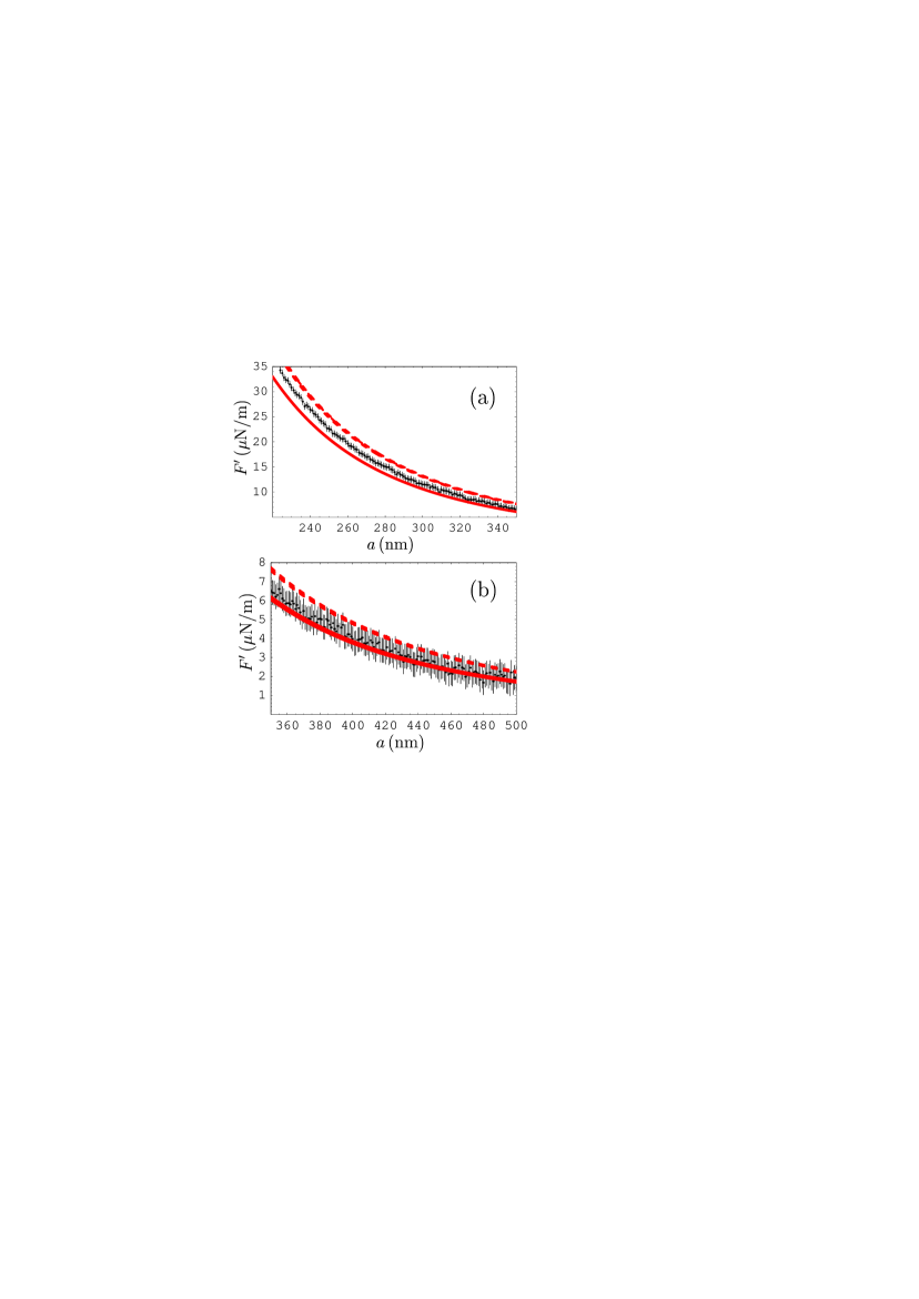
Figure 2: (Color online) The experimental data for the gradient of the Casimir force $F^{\prime}$ at (a) short and (b) long separations are shown as crosses plotted at a 67% confidence level (measured with the applied compensating voltage for the first sample). The theoretical $F^{\prime}$ between an Au-coated sphere and a Si-SiO₂ substrate calculated using the Lifshitz theory and between an Au-coated sphere and graphene deposited on this substrate calculated using an additive approach are shown as the solid and dashed bands, respectively.

                          

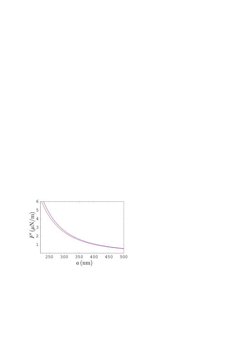
Figure 3: (Color online) The gradient of the Casimir force between an Au-coated sphere and a suspended graphene sheet calculated using the Dirac model with the mass gap parameter equal to 0.1 eV (lower line) and 0 (upper line) as a function of separation.

Table 1: The mean values of the gradient of the Casimir force together with their total experimental errors at different separations (first column) measured in this work with applied compensating voltage (column a) and with different applied voltages (column b) for the first graphene sample (columns c and d, respectively, for the second graphene sample). Columns e and f contain theoretical values for the gradients of the Casimir force between the Au sphere and Si-SiO₂ substrate calculated when Au and Si are described by the plasma and Drude model approaches, respectively.

	Gradients of the Casimir force $F^{\prime}\,(\mu\mbox{N/m})$
$a\,$(nm)	a	b	c	d	e	f
224	$34.27\pm 0.64$	$33.58\pm 0.65$	$34.12\pm 0.64$	$33.76\pm 0.65$	30.90	30.70
250	$22.62\pm 0.64$	$22.27\pm 0.64$	$22.72\pm 0.64$	$22.42\pm 0.64$	20.67	20.51
300	$11.50\pm 0.64$	$11.19\pm 0.64$	$11.65\pm 0.64$	$11.53\pm 0.64$	10.66	10.54
350	$6.52\pm 0.64$	$6.28\pm 0.64$	$6.30\pm 0.64$	$6.60\pm 0.64$	6.12	6.03
400	$3.98\pm 0.64$	$3.67\pm 0.64$	$3.99\pm 0.64$	$3.70\pm 0.64$	3.81	3.73
500	$1.90\pm 0.64$	$1.76\pm 0.64$	$1.78\pm 0.64$	$1.60\pm 0.64$	1.73	1.68

References

- (1) A. H. Castro Neto, F. Guinea, N. M. R. Peres, K. S. Novoselov, and A. K. Geim, Rev. Mod. Phys. 81, 109 (2009).
- (2) M. S. Dresselhaus, Physica Status Solidi (b) 248, 1566 (2011).
- (3) R. H. French, V. A. Parsegian, R. Podgornik et al., Rev. Mod. Phys. 82, 1887 (2010).
- (4) M. Bordag, J. Phys. A: Math. Gen. 39, 6173 (2006).
- (5) G. Gómes-Santos, Phys. Rev. B 80, 245424 (2009).
- (6) D. Drosdoff and L. M. Woods, Phys. Rev. B 82, 155459 (2010).
- (7) B. E. Sernelius, Europhys. Lett. 95, 57003 (2011).
- (8) J. Sarabadani, A. Naji, R. Asgari, and R. Podgornik, Phys. Rev. B 84, 155407 (2011).
- (9) G. L. Klimchitskaya and V. M. Mostepanenko, Phys. Rev. B 87, 075439 (2013).
- (10) M. Bordag, B. Geyer, G. L. Klimchitskaya, and V. M. Mostepanenko, Phys. Rev. B 74, 205431 (2006).
- (11) M. Bordag, I. V. Fialkovsky, D. M. Gitman, and D. V. Vassilevich, Phys. Rev. B 80, 245406 (2009).
- (12) I. V. Fialkovsky, V. N. Marachevsky, and D. V. Vassilevich, Phys. Rev. B 84, 035446 (2011).
- (13) D. Drosdoff and L. M. Woods, Phys. Rev. A 84, 062501 (2011).
- (14) M. Bordag, G. L. Klimchitskaya, and V. M. Mostepanenko, Phys. Rev. B 86, 165429 (2012).
- (15) A. D. Phan, L. M. Woods, D. Drosdoff, I. V. Bondarev, and N. A. Viet, Appl. Phys. Lett. 101, 113118 (2012).
- (16) E. V. Blagov, G. L. Klimchitskaya, and V. M. Mostepanenko, Phys. Rev. B 75, 235413 (2007).
- (17) Yu. V. Churkin, A. B. Fedortsov, G. L. Klimchitskaya, and V. A. Yurova, Phys. Rev. B 82, 165433 (2010).
- (18) T. E. Judd, R. G. Scott, A. M. Martin, B. Kaczmarek, and T. M. Fromhold, New. J. Phys. 13, 083020 (2011).
- (19) M. Chaichian, G. L. Klimchitskaya, V. M. Mostepanenko, and A. Tureanu, Phys. Rev. A 86, 012515 (2012).
- (20) A. Bogicevic, S. Ovesson, P. Hyldgaard, B. I. Lundqvist, H. Brune, and D. R. Jennison, Phys. Rev. Lett. 85, 1910 (2000).
- (21) E. Hult, P. Hyldgaard, J. Rossmeisl, and B. I. Lundqvist, Phys. Rev. B 64, 195414 (2001).
- (22) J. F. Dobson, A. White, and A. Rubio, Phys. Rev. Lett. 96, 073201 (2006).
- (23) A. N. Rudenko, F. J. Keil, M. I. Katsnelson, and A. I. Lichtenstein, Phys. Rev. B 84, 085438 (2011).
- (24) I. V. Bondarev and Ph. Lambin, Phys. Rev. B 70, 035407 (2004).
- (25) G. L. Klimchitskaya, U. Mohideen, and V. M. Mostepanenko, Rev. Mod. Phys. 81, 1827 (2009).
- (26) M. Bordag, G. L. Klimchitskaya, U. Mohideen, and V. M. Mostepanenko, Advances in the Casimir Effect (Oxford University Press, Oxford, 2009).
- (27) A. W. Rodriguez, F. Capasso, and S. G. Johnson, Nature Photon. 5, 211 (2011).
- (28) G. L. Klimchitskaya, U. Mohideen, and V. M. Mostepanenko, Int. J. Mod. Phys. B 25, 171 (2011).
- (29) C.-C. Chang, A. A. Banishev, G. L. Klimchitskaya, V. M. Mostepanenko, and U. Mohideen, Phys. Rev. Lett. 107, 090403 (2011).
- (30) C.-C. Chang, A. A. Banishev, R. Castillo-Garza, G. L. Klimchitskaya, V. M. Mostepanenko, and U. Mohideen, Phys. Rev. B 85, 165443 (2012).
- (31) A. A. Banishev, C.-C. Chang, G. L. Klimchitskaya, V. M. Mostepanenko, and U. Mohideen, Phys. Rev. B 85, 195422 (2012).
- (32) X. Li, C. W. Magnuson, A. Venugopal, R. M. Tromp, J. B. Hannon, E. M. Vogel, L. Colombo, and R. S. Ruoff, J. Amer. Chem. Soc. 133, 2816 (2011).
- (33) A. C. Ferrari, J. C. Meyer, V. Scardaci, C. Casiraghi, M. Lazzeri, F. Mauri, S. Piscanec, D. Jiang, K. S. Novoselov, S. Roth, and A. K. Geim, Phys. Rev. Lett. 97, 187401 (2006).
- (34) D. Graf, F. Molitor, K. Ensslin, C. Stampfer, A. Jungen, C. Hierold, and L. Wirtz, Nano Lett. 7, 238 (2007).
- (35) K. S. Novoselov, A. K. Geim, S. V. Morozov, D. Jiang, M. I. Katsnelson, I. V. Grigorieva, S. V. Dubonos, and A. A. Firsov, Nature 438, 197 (2005).
- (36) Y. Zhang, Y.-W. Tan, H. L. Stormer, and P. Kim, Nature 438, 201 (2005).
- (37) M. S. Tomaš, Phys. Rev. A 66, 052103 (2002).
- (38) C. D. Fosco, F. C. Lombardo, and F. D. Mazzitelli, Phys. Rev. D 84, 105031 (2011).
- (39) G. Bimonte, T. Emig, R. L. Jaffe, and M. Kardar, Europhys. Lett. 97, 50001 (2012).
- (40) G. Bimonte, T. Emig, and M. Kardar, Appl. Phys. Lett. 100, 074110 (2012).
- (41) Handbook of Optical Constants of Solids, ed. E. D. Palik (Academic, New York, 1985).
- (42) G. L. Klimchitskaya, U. Mohideen, and V. M. Mostepanenko, J. Phys.: Condens. Matter 24, 424202 (2012).
- (43) F. Chen, U. Mohideen, G. L. Klimchitskaya, and V. M. Mostepanenko, Phys. Rev. A 72, 020101(R) (2005); 74, 022103 (2006).
- (44) Handbook of Optical Constants of Solids, vol II, ed. E. D. Palik (Academic, New York, 1991).
- (45) L. Bergström, Adv. Colloid Interface Sci. 70, 125 (1997).
- (46) R. Podgornik, R. H. French, and V. A. Parsegian, J. Chem. Phys. 124, 044709 (2006).