Non-perturbative laser effects on the electrical properties of graphene nanoribbons

Abstract

The use of Floquet theory combined with a realistic description of the electronic structure of illuminated graphene and graphene nanoribbons is developed to assess the emergence of non-adiabatic and non-perturbative effects on the electronic properties. Here, we introduce an efficient computational scheme and illustrate its use by applying it to graphene nanoribbons in the presence of both linear and circular polarization. The interplay between confinement due to the finite sample size and laser-induced transitions is shown to lead to sharp features on the average conductance and density of states. Particular emphasis is given to the emergence of the bulk limit response.

1 Introduction

Carbon-based materials such as graphene and carbon nanotubes constitute a privileged family of novel nanomaterials with outstanding properties [1, 2, 3]. Within this playground, graphene optics and optoelectronics has become one of the most exciting areas for research [4, 5, 6]. Besides being one of the best tools for non-invasive characterization and probing of carbon-based materials [7], light can also be used as means for achieving new functions such as improved energy harvesting [8], or novel plasmonic properties [9, 10] and there are big expectations that we are going to have even more in the coming years. At the core of these phenomena we are confronted with fundamental aspects of the interaction between light and matter in low dimensionality.

While the effects of light and other bosonic excitations on the electronic properties is usually treated within a Fermi Golden rule and/or adiabatic approximations, their breakdown is indeed a possibility in the graphene flatland [11, 12], as demonstrated by some remarkable experiments [13].

The illumination with a laser was also proposed to lead to non-perturbative and non-adiabatic effects in graphene including the opening of a bandgap [14] owing to photon-assisted coupling between electronic states at half the photon energy, i.e. $\pm\hbar\Omega/2$. Further studies pointed out that circularly polarized light may also lead to a Hall effect without a static magnetic field: the photovoltaic Hall effect [15] which lacks an experimental confirmation.

These puzzling possibilities attracted much attention [16, 17, 18] and recent atomistic simulations of the dc electrical response hint that a laser in the mid-infrared would be optimal for experimental verification [16]. Further studies focused on the optical response [17, 19] as well as other interesting issues [20, 21, 22, 23]. Recently, the possibility of inducing topologically protected states by laser illumination in semiconductors [24] and both in monolayer [25, 26] and bilayer [27] graphene has become a hot field [28, 29] with an impact on other areas such as condensates [30] and photonic crystals, where experiments are already available [31].

Most of the results mentioned before have been derived for bulk monolayer graphene (bilayer graphene was also studied in [32, 27]) and only few results are available for the case of graphene nanoribbons [26, 33]. In this paper, we extend over our previous results [33] giving a more comprehensive and in-depth view of the numerical scheme used and the interplay between lateral confinement and photon-assisted processes in illuminated graphene nanoribbons. To this end, we apply Floquet theory to a nearest neighbor tight-binding model to describe the $\pi$-orbitals around the Fermi energy in presence of a time-periodic field. In this approach, the average density of states (DOS) and the dc component of the conductance are calculated through an efficient reduction of the Floquet Hamiltonian by a recursive decimation procedure [34]. The power of this technique allows us to explore the electrical properties of the system in a wide range of parameters, including arbitrary edge geometries and ribbon sizes as well as different laser polarizations.

As will be made clear in the next sections, the non-perturbative character of the field is revealed through a strong dependence in the laser-induced gaps with respect to the direction of the polarization. In addition to the known dynamical gaps developed at $\pm\hbar\Omega/2$ [14], further modifications in the DOS emerge as a consequence of the inter-mode coupling induced by the laser. The effect is discussed in both armchair and zigzag nanoribbons for different orientations of the radiation field. Finally, for large nanoribbons the effects of both linear and circular polarizations are also discussed. We show how the above modifications in the DOS average out around $\pm\hbar\Omega/2$, thereby recovering the known solution in the bulk limit [14, 15].

Our work is organized as follows. In section 2 we introduce the considered model and give a detailed overview of the simulation scheme. Section 3 is devoted to the discussion of our results. Finally, we present our conclusions in section 4.

2 Simulation scheme: Floquet theory applied to illuminated graphene nanoribbons

In this section we outline the approach used to investigate the effects of the laser field in the electronic structure and transport properties of graphene nanoribbons. Our starting point is the description of the $\pi$-orbital electrons through the following tight-binding Hamiltonian

$$\hat{\mathcal{H}}(t)=\sum_{i}\epsilon_{i}\hat{c}_{i}^{\dagger}\hat{c}_{i}-\sum_{\braket{i,j}}\gamma_{ij}(t)\hat{c}_{i}^{\dagger}\hat{c}_{j},$$ (1)

where $\hat{c}_{i}^{\dagger}(\hat{c}_{i})$ creates (annihilates) an electron at site $i$ and the sum in the second term only takes pairs of nearest-neighbor sites. The potential energy induced by, e.g., a gate voltage or local impurities, is represented by the on-site energies $\epsilon_{i}$ while the hopping term $\gamma_{ij}$ gives the transition amplitude between sites $i$ and $j$.

The time-dependent field is considered by neglecting the small magnetic component and with an electric field which is written in a Weyl’s gauge in terms of a vector potential: $\mathbf{E}=-\partial\mathbf{A}/\partial t$. The vector potential is included through the Peierls substitution [35], which introduces an additional phase in the hopping amplitude connecting two adjacent sites $i$ and $j$, i.e.

$$\gamma_{ij}(t)=\gamma_{0}\exp\left[i\frac{2\pi}{\Phi_{0}}\int_{\mathbf{r}_{j}}^{\mathbf{r}_{i}}\mathbf{A}(t)\cdot d\mathbf{r}\right],$$ (2)

where $\gamma_{0}=2.7\,\mathrm{eV}$ is the typical hopping amplitude at zero field [3] and $\Phi_{0}$ is the magnetic flux quantum. For monochromatic waves, the gauge potential related to the time-dependent electric field is defined as

$$\mathbf{A}(t)=A_{0}\left[\cos\beta\cos(\Omega t)\mathbf{x}+\sin\beta\cos(\Omega t-\varphi)\mathbf{y}\right],$$ (3)

where $A_{0}=E_{0}/\Omega$ and $E_{0}$ is the amplitude of the electric field. The direction and polarization of the field are fixed by the parameters $\beta$ and $\varphi$, respectively. In the next section we will concentrate on three paradigmatic cases, namely, linear polarization along either the (longitudinal) $x$-axis or (transversal) $y$-axis and circular polarization.

To deal with the time-dependence in the electronic hopping terms, we use Floquet theorem [36, 37]. In the next subsection, the Floquet Hamiltonian accounting for the $2\pi/\Omega$-periodic real-space Hamiltonian is discussed in detail together with the employed technique for the derivation of the observables (DOS and conductance) which are investigated.

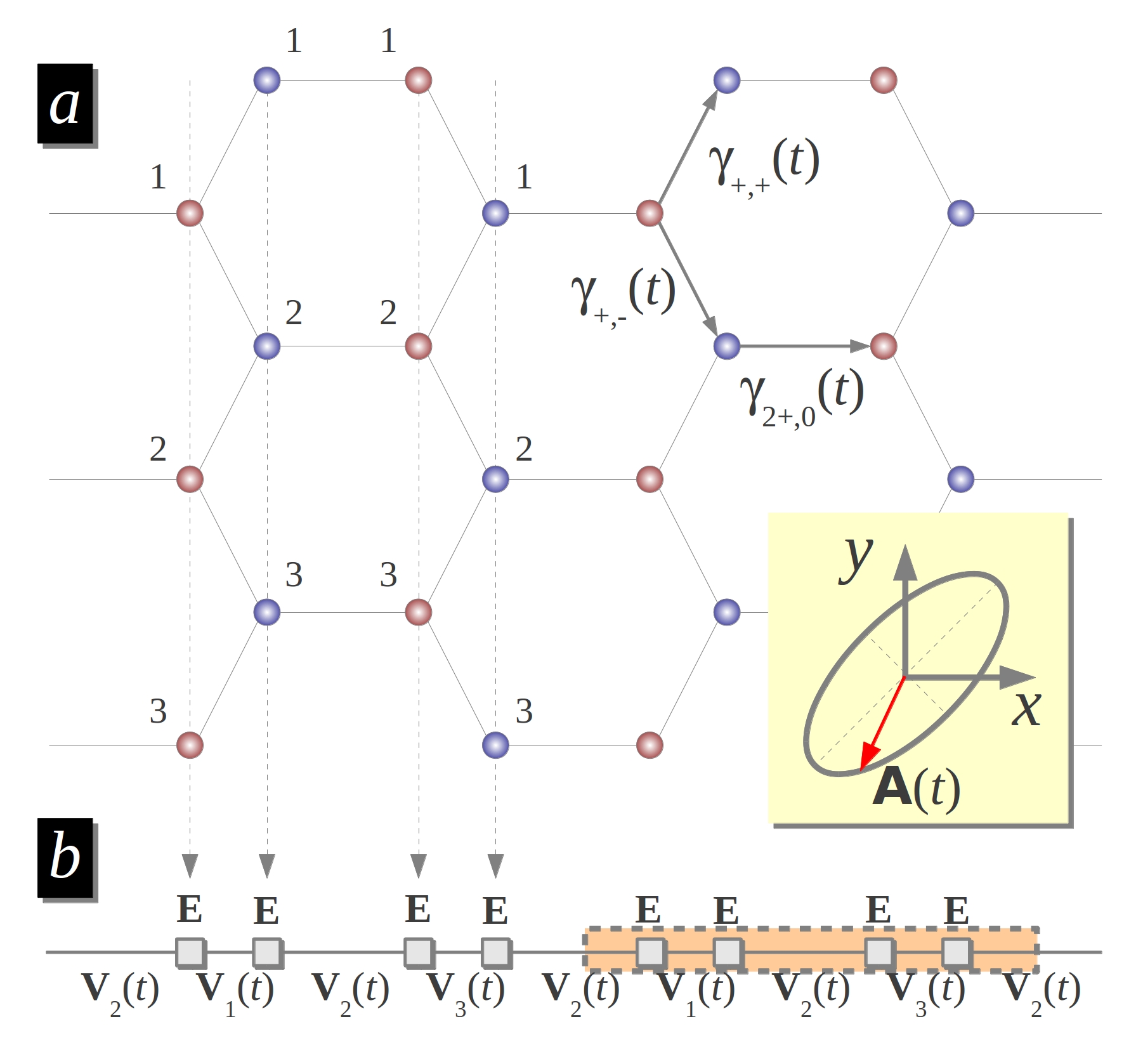
Figure 1: (a) Scheme of the considered model for the example of an armchair nanoribbon. The laser field is applied perpendicular to the lattice and defines the time-dependent hoppings $\gamma_{+,+}(t),\gamma_{+,-}(t)$ and $\gamma_{2+,0}(t)$. (b) Representation of the real-space Hamiltonian in terms of diagonal blocks $\mathbf{E}$ and hopping matrices $\mathbf{V}_{i}(t)$. The unit cell for the case of an armchair nanoribbon is indicated by a rectangle.

2.1 Determination of the matrix elements of the Floquet Hamiltonian

A scheme of the considered system is shown in figure 1(a), where the phases of the hopping amplitudes account for the time-dependent vector potential associated to the laser. For two adjacent (transversal) arrays in the lattice, we consider the hopping amplitudes always going from left to right. With the assumption that the electric field is uniform along the whole sample, the phases in equation 2 are given by the scalar product between the vector potential and the vector $\mathbf{r}_{ij}=\mathbf{r}_{i}-\mathbf{r}_{j}$ connecting the two sites. This allows to fully describe the system in terms of three possible orientations of the vector $\mathbf{r}_{ij}$, i.e., $\mathbf{r}_{ij}=a(\cos\alpha_{ij},\sin\alpha_{ij})$, with $a\simeq 0.142\,\mathrm{nm}$ the distance between nearest-neighbor carbon atoms and $\alpha_{ij}=0,\pm\pi/3$. For these orientations, the hopping elements are

$$\gamma_{2+,0}(t) = \gamma_{0}e^{i2z_{x}\cos(\Omega t)},$$ (4)

$$\gamma_{+,\pm}(t) = \gamma_{0}e^{i(z_{x}\pm z_{y}\cos\varphi)\cos(\Omega t)}e^{\pm iz_{y}\sin\varphi\sin(\Omega t)},$$ (5)

respectively, where the indices are now related to the $x$ and $y$ components of the vectors connecting the carbon atoms. To simplify the notation, we define adimensional variables $z_{x}=\pi aA_{0}\cos\beta/\Phi_{0}$ and $z_{y}=\sqrt{3}\pi aA_{0}\sin\beta/\Phi_{0}$ which quantify the relative strength of the laser.

We divide the real-space Hamiltonian in diagonal blocks $\mathbf{E}$ accounting for the on-site energies in the lattice which belong to the same transversal array. In homogeneous samples, they are simply zero, i.e. $\mathbf{E}=\mathbf{0}$. The hopping matrices $\mathbf{V}_{i}(t)$ connecting the arrays alternate periodically depending on the particular position in the unit cell (see figure 1(b)). The dimension of these block matrices is given by the number $N$ of carbon atoms along the transversal direction.

A Fourier decomposition of the time-dependent Hamiltonian spans the real space into a composite space $\mathcal{R}\times\mathcal{T}$ including the $2\pi/\Omega$-periodic functions [36, 37]. The basis of this Floquet space is conformed by the states $\ket{i,n}$, where the first index labels the site location of the sites and the second, the Fourier index, indicates the number of photons. The resulting time-independent (Floquet) Hamiltonian $\mathbf{H}_{F}$ is determined by the hopping elements connecting the states $\ket{i,n}$ and $\ket{j,n+m}$

$$\gamma_{+,\pm}^{m} = \gamma_{0}\sum_{k=-\infty}^{\infty}i^{k}J_{k}(z_{x}\pm z_{y}\cos\varphi)J_{m-k}(\pm z_{y}\sin\varphi),$$ (6)

$$\gamma_{2+,0}^{m} = \gamma_{0}i^{m}J_{m}(2z_{x}),$$ (7)

where $J_{n}(z)$ is the Bessel function of order $n$. In contrast to similar treatments of the periodic time-dependent field based on the k.p approach [14, 15], the present calculations may involve transitions with more than a single photon. However, for the mid-infrared regime ($\hbar\Omega\simeq 140\,\mathrm{meV}$) and laser power ($P=1-10\,\mathrm{mW/\mu m^{2}}$) considered here we have $z_{x},z_{y}\ll 1$, such that these transitions decay rapidly and the leading contributions still come from the renormalization of the hoppings ($m=0$) and inelastic transitions with a single photon ($m=\pm 1$). The method is here illustrated for the specific case of armchair nanoribbons, but the same strategy can be easily adapted to other edge geometries.

Now that we have an explicit expression for the hopping amplitudes, we can compute the Floquet Hamiltonian by noticing that each block in figure 1(b) is splitted into $2N_{F}+1$ “replicas” accounting for states with different Fourier index. In this sense, $N_{F}$ denotes the maximum number of considered Fourier modes and dictates the truncation of the total Floquet space. The on-site energies in the diagonal blocks are given as a multiple integer of the photon energy, i.e., $\epsilon_{i,n}=n\hbar\Omega$, with $n=-N_{F},\dots,N_{F}$. According to this Fourier expansion, the structure of the Floquet Hamiltonian can be understood as a block tridiagonal matrix where each block is of dimension $(2N_{F}+1)N$. The diagonal blocks $\mathbf{E}_{F}$ include the arrays with different Fourier index. This group of arrays then form a layer and the off-diagonal blocks contain the hopping amplitudes connecting them. Since in our representation each layer contains carbon atoms belonging to the same sublattice ($A$ or $B$), the matrix elements of the diagonal blocks simply read $\bra{i,n}\mathbf{E}_{F}\ket{j,m}=n\hbar\Omega\delta_{ij}\delta_{nm}$. For off-diagonal blocks, however, we need to distinguish three different hopping matrices $\mathbf{V}_{F,k}$, with $k=1,2$ or $3$, according to which layers they interconnect. To account for transitions with different number of photons, each matrix is divided, in turn, into $2N_{F}+1$ submatrices such that $\bra{i,n}\mathbf{V}_{F,k}\ket{j,n+m}=\bra{i}\mathbf{V}_{k}^{m}\ket{j}$, where

$$\mathbf{V}_{1}^{m} = \left(\begin{array}[]{ccc}\gamma_{+,+}^{m}&\gamma_{+,-}^{m}&\\ 0&\gamma_{+,+}^{m}&\\ &&\ddots\end{array}\right),\mathbf{V}_{2}^{m}=\left(\begin{array}[]{ccc}\gamma_{2+,0}^{m}&0&\\ 0&\gamma_{2+,0}^{m}&\\ &&\ddots\end{array}\right),$$ (14)

$$\mathbf{V}_{3}^{m} = \left(\begin{array}[]{ccc}\gamma_{+,-}^{m}&0&\\ \gamma_{+,+}^{m}&\gamma_{+,-}^{m}&\\ &&\ddots\end{array}\right).$$ (18)

This representation of the Floquet Hamiltonian constitutes our starting point in the analysis of the electronic properties of the ribbons in the presence of a time-dependent field. In previous works [16], the particular case of armchair nanoribbons illuminated by linearly polarized light along the longitudinal direction was intensively studied. This was motivated by the fact that this geometry allows for a convenient decomposition of the Floquet Hamiltonian into normal modes, thereby making it a suitable model to analyze the bulk limit for a large lateral size of the ribbon. In the next section, however, we will concentrate first on relatively small sized ribbons, and our efforts will be devoted to investigate the role of the laser field in the characteristics of the electronic structure due to lateral confinement. After discussing the interplay between these two effects, we will explore the bulk limit for different directions of the linear polarization and also for circularly polarized fields.

2.2 Density of states and Conductance

We now comment on the quantities of interest that we want to address in the next section when taking specific values for the size and edge geometry of the ribbons as well as tuning the laser field. Starting from the above mentioned Floquet Hamiltonian, it is possible to define the retarded Floquet-Green functions according to [38, 39]

$$\mathbf{G}_{\mathrm{F}}(\varepsilon)=\left(\varepsilon\mathbf{1}-\mathbf{H}_{\mathrm{F}}\right)^{-1}.$$ (19)

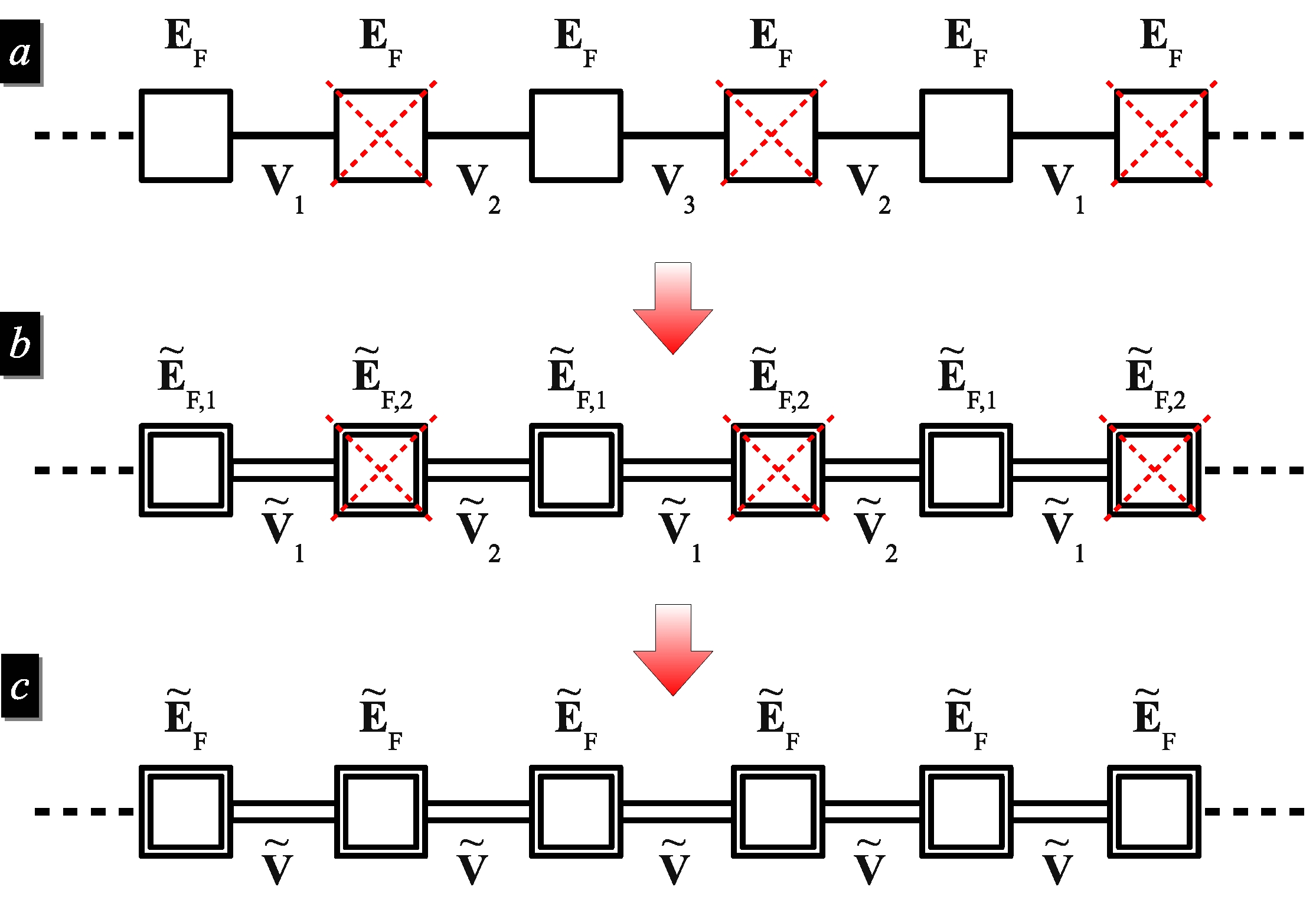
Figure 2: Decimation procedure in Floquet space. (a) Effective representation of $\mathbf{H}_{F}$. Dashed red crossing lines denote the reduced blocks. (b) Effective Hamiltonian after one step: The diagonal block matrices $\tilde{\mathbf{E}}_{F,i}$ and the effective hopping matrices $\tilde{\mathbf{V}}_{i}$ are renormalized by the reduced blocks. (c) Homogeneous effective Hamiltonian after the second step of the decimation procedure.

Since we want to analyze how the electronic properties of the ribbon are affected by the laser, we refer to the average density of states (DOS) obtained after tracing over the sites with zero photon, i.e.

$$\mathcal{N}_{0}(\varepsilon)=-\frac{1}{\pi}\lim_{\eta\rightarrow 0}\mathrm{Im}\left[\sum_{i=1}^{N}\bra{i,0}\mathbf{G}_{F}(\varepsilon+i\eta)\ket{i,0}\right],$$ (20)

where the (imaginary) regularization energy $i\eta$ is carefully chosen to reach the thermodynamical limit along the longitudinal direction. A “brute-force” calculation of the inverse of the Floquet Hamiltonian could in principle represent a hard (or even impossible) task when considering the full system. However, the decimation technique [40, 34], based on the recursive calculation of the self-energy correction $\mathbf{\Sigma}_{F}(\varepsilon)$ to the diagonal block matrices, constitutes an appropriate strategy to circumvent this hurdle. Figure 2 shows a scheme where the Floquet Hamiltonian is represented by an effective linear chain. Here, the squares correspond to the diagonal blocks $\mathbf{E}_{F}$, which are connected through the hopping matrices $\mathbf{V}_{i}$. In this procedure, we calculate the effective Hamiltonian resulting from the systematic elimination of blocks in the lattice (dashed red crossing lines in the figure). This reduction of the basis along the longitudinal direction leads to a renormalization of both the diagonal blocks and hopping matrices. According to figure 2, after the first decimation step (panel $b$), these read

$$\tilde{\mathbf{E}}_{F,1} = \mathbf{E}_{F}+\mathbf{V}_{1}\frac{1}{\varepsilon\mathbf{1}-\mathbf{E}_{F}}\mathbf{V}_{1}^{\dagger}+\mathbf{V}_{2}^{\dagger}\frac{1}{\varepsilon\mathbf{1}-\mathbf{E}_{F}}\mathbf{V}_{2},$$ (21)

$$\tilde{\mathbf{E}}_{F,2} = \mathbf{E}_{F}+\mathbf{V}_{3}\frac{1}{\varepsilon\mathbf{1}-\mathbf{E}_{F}}\mathbf{V}_{3}^{\dagger}+\mathbf{V}_{2}^{\dagger}\frac{1}{\varepsilon\mathbf{1}-\mathbf{E}_{F}}\mathbf{V}_{2},$$ (22)

$$\tilde{\mathbf{V}}_{1} = \mathbf{V}_{1}\frac{1}{\varepsilon\mathbf{1}-\mathbf{E}_{F}}\mathbf{V}_{2},$$ (23)

$$\tilde{\mathbf{V}}_{2} = \mathbf{V}_{3}\frac{1}{\varepsilon\mathbf{1}-\mathbf{E}_{F}}\mathbf{V}_{2}.$$ (24)

The next step in the recursion consists of the reduction of the blocks with $\tilde{\mathbf{E}}_{F,2}$, and provides an homogeneous effective Hamiltonian (panel $c$) with diagonal blocks and hopping matrices renormalized by

$$\tilde{\mathbf{E}}_{F} = \tilde{\mathbf{E}}_{F,1}+\tilde{\mathbf{V}}_{1}\frac{1}{\varepsilon\mathbf{1}-\tilde{\mathbf{E}}_{F,2}}\tilde{\mathbf{V}}_{1}^{\dagger}+\tilde{\mathbf{V}}_{2}^{\dagger}\frac{1}{\varepsilon\mathbf{1}-\tilde{\mathbf{E}}_{F,2}}\tilde{\mathbf{V}}_{2},$$ (25)

$$\tilde{\mathbf{V}} = \tilde{\mathbf{V}}_{1}\frac{1}{\varepsilon\mathbf{1}-\tilde{\mathbf{E}}_{F,2}}\tilde{\mathbf{V}}_{2}.$$ (26)

By repeating this process $M$ times, the self-energy correction to the diagonal block $\mathbf{E}_{F}$ accounts for a system with $2^{M}$ layers along the longitudinal direction. Therefore, the DOS reduces to

$$\mathcal{N}_{0}(\varepsilon)=-\frac{1}{\pi}\lim_{\eta\rightarrow 0}\sum_{i=1}^{N}\mathrm{Im}\bra{i,0}\frac{1}{(\varepsilon+i\eta)\mathbf{1}-\mathbf{E}_{F}-\mathbf{\Sigma}_{F}}\ket{i,0},$$ (27)

which only involves the inversion of a single block matrix.

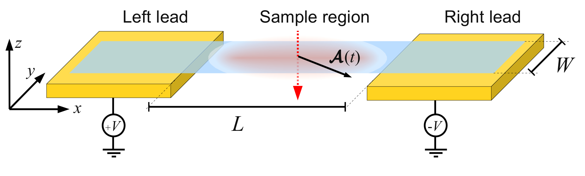
Figure 3: (Color online) Scheme of the transport setup. The graphene nanoribbon is coupled to two metallic reservoirs. The central region (sample) is illuminated by a laser field perpendicular to the plane of the ribbon.

The above scheme is also of great help for an efficient evaluation of the dc component of the conductance. In this case we imagine a situation as the one represented on figure 3, where only a finite region of space is affected by the laser (“the sample”). If we consider the rest as reservoirs, then we can compute the Floquet-Green functions for the sample by representing the $\alpha$-electrode ($\alpha=L,R$) through a self-energy correction $\mathbf{\Sigma}_{\alpha}=\mathbf{\Delta}_{\alpha}-i\mathbf{\Gamma}_{\alpha}$ as usual. How are these Green’s functions connected to the dc current? For non-interacting electrons, the average (coherent) current over a period of the modulation is given by:

$$\bar{I}=\frac{2e}{h}\sum_{n}\int\left[T_{R\leftarrow L}^{(n)}(\varepsilon)f_{L}(\varepsilon)-T_{L\leftarrow R}^{(n)}(\varepsilon)f_{R}(\varepsilon)\right]d\varepsilon,$$ (28)

where $T_{R\leftarrow L}^{(n)}(\varepsilon)$ are the transmission probabilities from the left ($L$) to the right ($R$) reservoirs involving the emission/absorption of $n$ photons. These probabilities can be written in terms of the Floquet-Green functions for the system [37, 41]:

$$T_{R\leftarrow L}^{(n)}(\varepsilon)=\Tr\left[2\mathbf{\Gamma}_{R,n}(\varepsilon)\mathbf{G}_{(R,n)\leftarrow(L,0)}(\varepsilon)2\mathbf{\Gamma}_{L,0}(\varepsilon)\mathbf{G}^{{\dagger}}_{(R,n)\leftarrow(L,0)}(\varepsilon)\right],$$ (29)

where $\mathbf{G}_{(R,n)\leftarrow(L,0)}(\varepsilon)$ is the block matrix for the Floquet-Green function connecting the left and right electrodes with the exchange of $n$ photons. Here the subindex $F$ was omitted to simplify the notation. As a consequence of the thermodynamical limit, the coupling to the (open) leads (see figure 3) implies a decay rate in the states within the sample which is accounted by

$$\mathbf{\Gamma}_{\alpha,n}(\varepsilon)=-\mathrm{Im}\left[\mathbf{\Sigma}_{\alpha}(\varepsilon+n\hbar\Omega)\right].$$ (30)

Since we assume a laser affecting only the sample region, these terms can be computed in terms of the “bare” self-energy correction $\mathbf{\Sigma}_{\alpha}(\varepsilon)$ obtained in the absence of time-dependent fields. The calculation of the current is thus completed by assuming that the asymptotic occupation in the leads, where no inelastic processes are allowed, is given by the usual Fermi functions

$$f_{\alpha}(\varepsilon)=\frac{1}{1+e^{\beta(\varepsilon-\mu_{\alpha})}},$$ (31)

where $\mu_{\alpha}$ is the electrochemical potential in the $\alpha$-lead and $\beta$ the inverse temperature.

3 Results

In this section we apply the discussed method to investigate modifications in the electronic properties of graphene nanoribbons induced by a laser field. In particular, we scrutinize the case of a laser within the mid-infrared region of the spectrum, where photon energies can be made smaller than the typical optical phonon energy while keeping the laser power small ($1-10\,\mathrm{mW/\mu m^{2}}$). By an appropriate tuning of the Fermi energy and polarization of the laser, we show how one can dramatically change the electrical and transport properties of the ribbons. This is illustrated for different sizes and edge geometries of the ribbons.

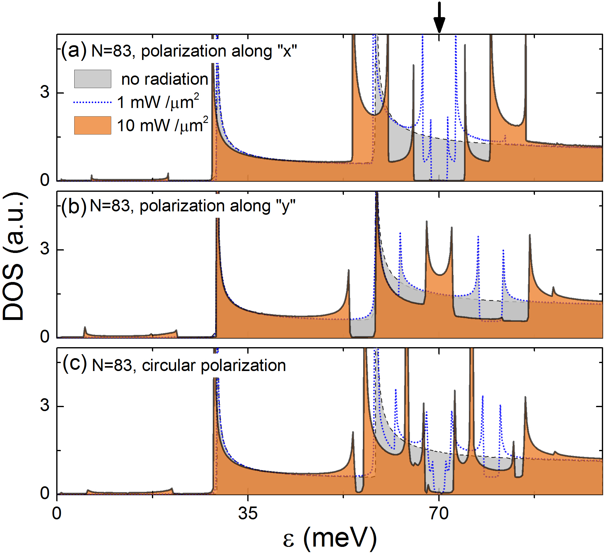
Figure 4: (Color online) Average density of states for an armchair graphene nanoribbon with $N=83$ in the presence of linearly polarized radiation along the $x$ direction (a), $y$ (b) and circular polarization (c).

Figure 4 shows the DOS (cf. equation 27) for an armchair ribbon with $N=83$ as a function of the Fermi energy. Three cases are analyzed: (a) linear polarization along $x$, (b) linear polarization along $y$, and (c) circular polarization. The energy of the laser is fixed to $\hbar\Omega=140\,\mathrm{meV}$, such that modifications in the DOS are expected to occur in the vicinity of the energy $\varepsilon\simeq 70\,\mathrm{meV}$ (marked by an arrow on the top panel).

In panel $a$, we observe that the interaction with the laser leads to a gap formation around $\varepsilon=\hbar\Omega/2$. The occurrence of this gap is related to an inelastic backscattering process that enables transitions between quasi-states in the Floquet spectrum. In this picture, each mode contains a series of replicas accounting for excitation states with different number of photons. In presence of linearly polarized light along $x$, the electronic states are connected to (photoexcited) hole states which belong to the same mode. Since electron-hole symmetry is now preserved along the point $n\hbar\Omega$ for a replica with $n$ photons, the energy values at which the gap may form are commensurate with $\hbar\Omega/2$. Additionally, the width of the gap is shown to be sensitive to the transversal direction of the momentum operator, such that it increases with the allowed values of $k_{y}$. This can be observed in the structure of the DOS around $\varepsilon=\hbar\Omega/2$, where two concentric gaps are developed, each one of them related to a different mode.

In panel $b$, one can observe that the DOS is drastically changed. Here the dynamical gap around $\varepsilon=\hbar\Omega/2$ is suppressed and two “satellite” depletion regions, where the DOS is diminished, appear instead. Depending on the particular normal mode affected by the field, these depletions may or not develop as a true gap. For a laser power $P=10\,\mathrm{mW/\mu m^{2}}$ (solid line), the left depletion is crossed by a van Hove singularity and a gap is opened in the region of the first semiconductor band.

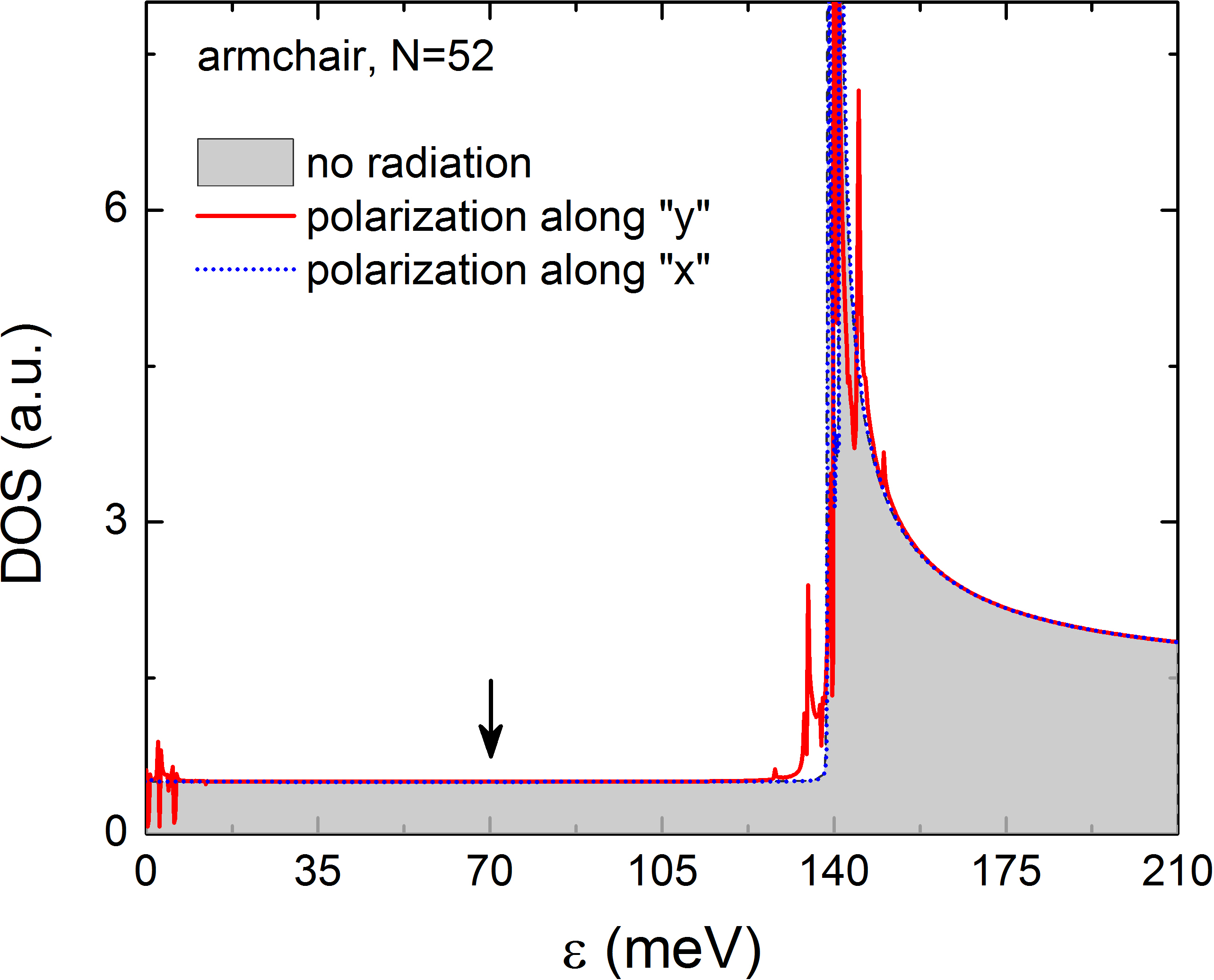
Figure 5: (Color online) Average density of states for a metallic armchair nanoribbon $N=52$ in the presence of linearly polarized radiation ($\hbar\Omega=140\,\mathrm{meV},P=1\,\mathrm{mW/\mu m^{2}}$) along the $y$ direction (solid red) and $x$ direction (dotted blue).

Of particular interest is the case of a metallic armchair nanoribbon, as shown in figure 5. Here the DOS around $\varepsilon=\hbar\Omega/2$ is completely immune to the influence of the laser, such that no bandgaps appear regardless of the particular direction of the polarization.

The above features observed in figures 4(a) and 4(b) can be combined if the laser field points along any intermediate direction between the $x$ and $y$ axes. This is shown in panel $c$ where a circularly polarized field is considered. Although for small samples this last case produces similar modifications in the DOS as compared to linear polarization along the direction $\mathbf{x+y}$, in the bulk limit these two cases become qualitatively different.

As mentioned in section 3, the developed technique is not necessarily restricted to armchair ribbons and can be easily adapted to other edge geometries. In figure 6 we show the DOS for a zigzag nanoribbon with $N=250$. Compared to figure 4, the features in the DOS observed in the armchair case are also present here. The difference now comes from the change in the relative angle between the lattice orientation and the direction of the polarization. In this sense, dynamical gaps around $\pm\hbar\Omega/2$ occur now for a laser along the $y$-direction. In addition, one can observe small depletions at both sides of the gap which can be related to the laser-induced coupling between different normal modes. We will come back to this point below. By changing the polarization direction to the $x$-axis, the dynamical gap is again suppressed and several depletion regions appear.

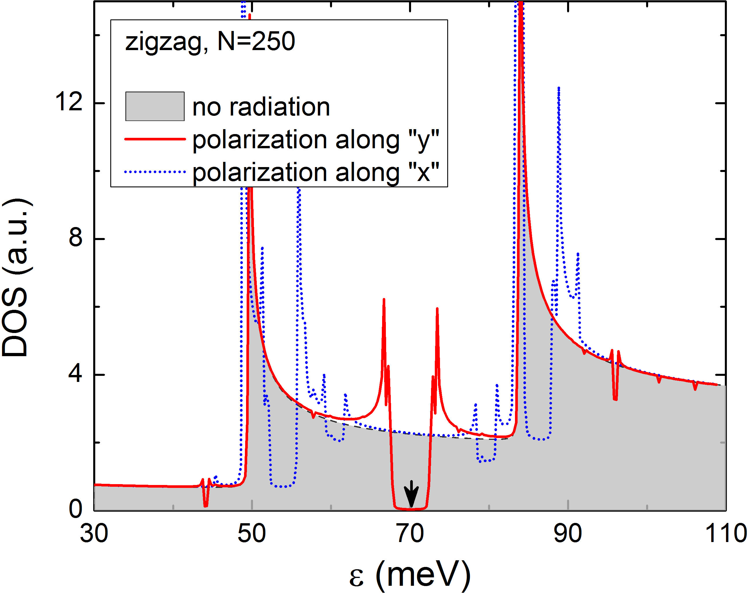
Figure 6: (Color online) Average density of states for a zigzag nanoribbon with $N=250$ in the presence of linearly polarized radiation ($\hbar\Omega=140\,\mathrm{meV}$) along the $y$-direction (solid red) and $x$-direction (dotted blue) for a laser power $P=1\,\mathrm{mW/\mu m^{2}}$.

An analysis of the bulk situation [15, 16] would only predict laser-induced depletions or gaps at $\pm n\hbar\Omega/2$ and no dependence on the linear polarization direction. Natural questions are therefore: why do these features away from $\pm n\hbar\Omega/2$ emerge? How do we reach the bulk limit?

Two different kind of processes are at the heart of these phenomena: intra-mode and inter-mode photon-induced transitions. For intra-mode transitions, both the initial and the final electronic states belong to the same transversal mode and the coupled states are located symmetrically with respect to the charge neutrality point which leads to the gaps or depletions at $\pm n\hbar\Omega/2$.

In contrast, inter-mode transitions couple states that are not symmetrically located around the Dirac point. In armchair ribbons, this is evident for the case of polarization in the $y$-direction, where it turns out that inter-mode transitions are the only allowed processes. Therefore, the polarization direction can be used to tune the relative magnitude of the different kind of processes: intra and inter mode.

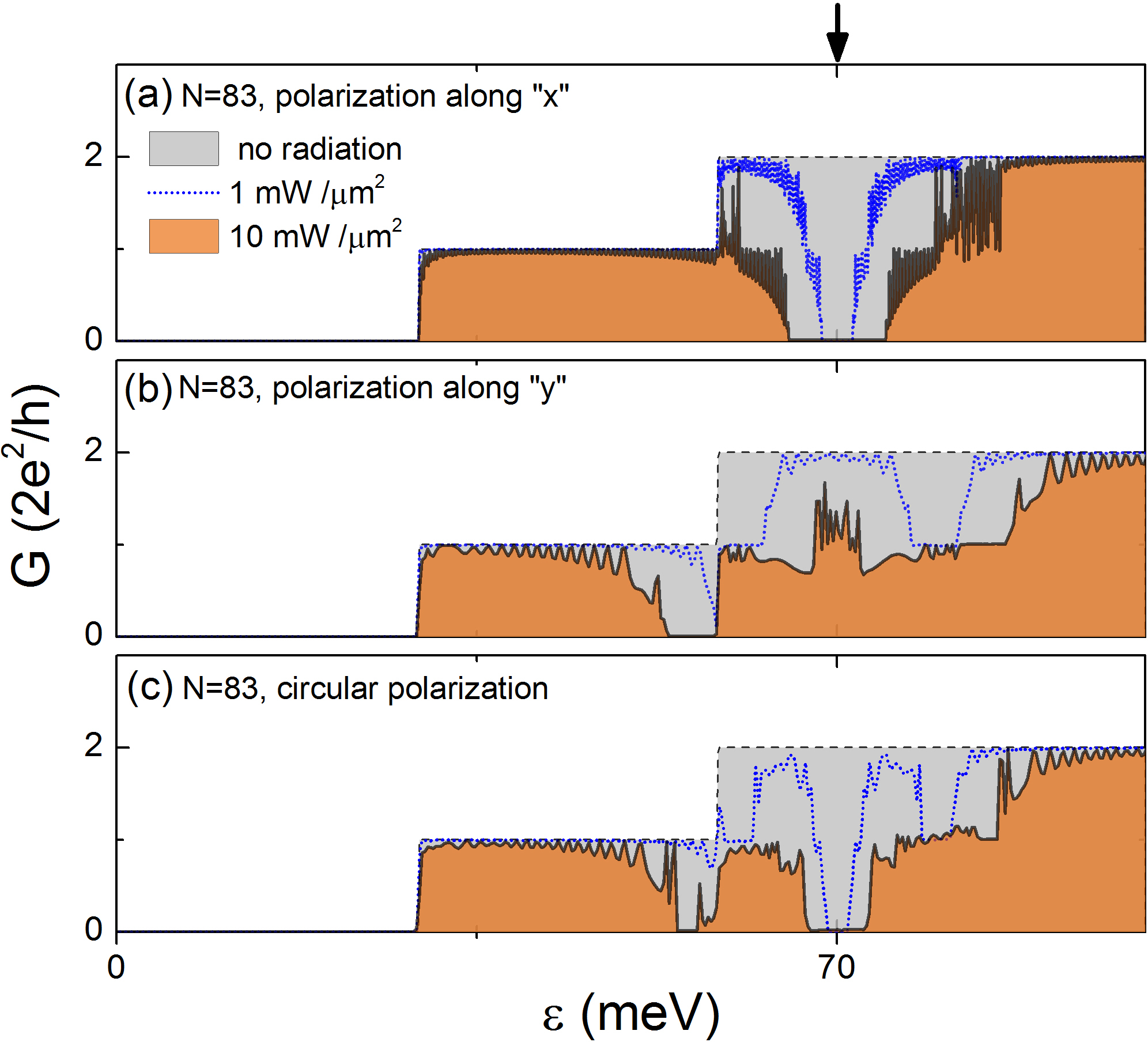
Figure 7: (Color online) DC component of the conductance for an armchair graphene nanoribbon with $N=83$ in the presence of linearly polarized radiation along the $x$ direction (a), $y$ (b) and circular polarization (c).

We now calculate the dc component of the conductance at zero temperature. When $T_{R\leftarrow L}^{(n)}(\varepsilon)=T_{L\leftarrow R}^{(n)}(\varepsilon)$, it is straightforward to show (cf. equation 29) that the conductance reduces to:

$$G(\varepsilon)=\frac{2e^{2}}{h}\sum_{n}T_{R\leftarrow L}^{(n)}(\varepsilon).$$ (32)

We use this expression, neglecting the small quantum pumping component ($\left|T_{R\leftarrow L}-T_{L\leftarrow R}\right|\ll T_{R\leftarrow L}$).

Figure 7 shows the conductance for the same set of parameters as in figure 4. One observes that the same qualitative features also appear in this case. By comparing the panels in the figure one sees that the direction of the polarization may be used as a “knob” to turn on or off the conductance at appropriate values of the Fermi energy.

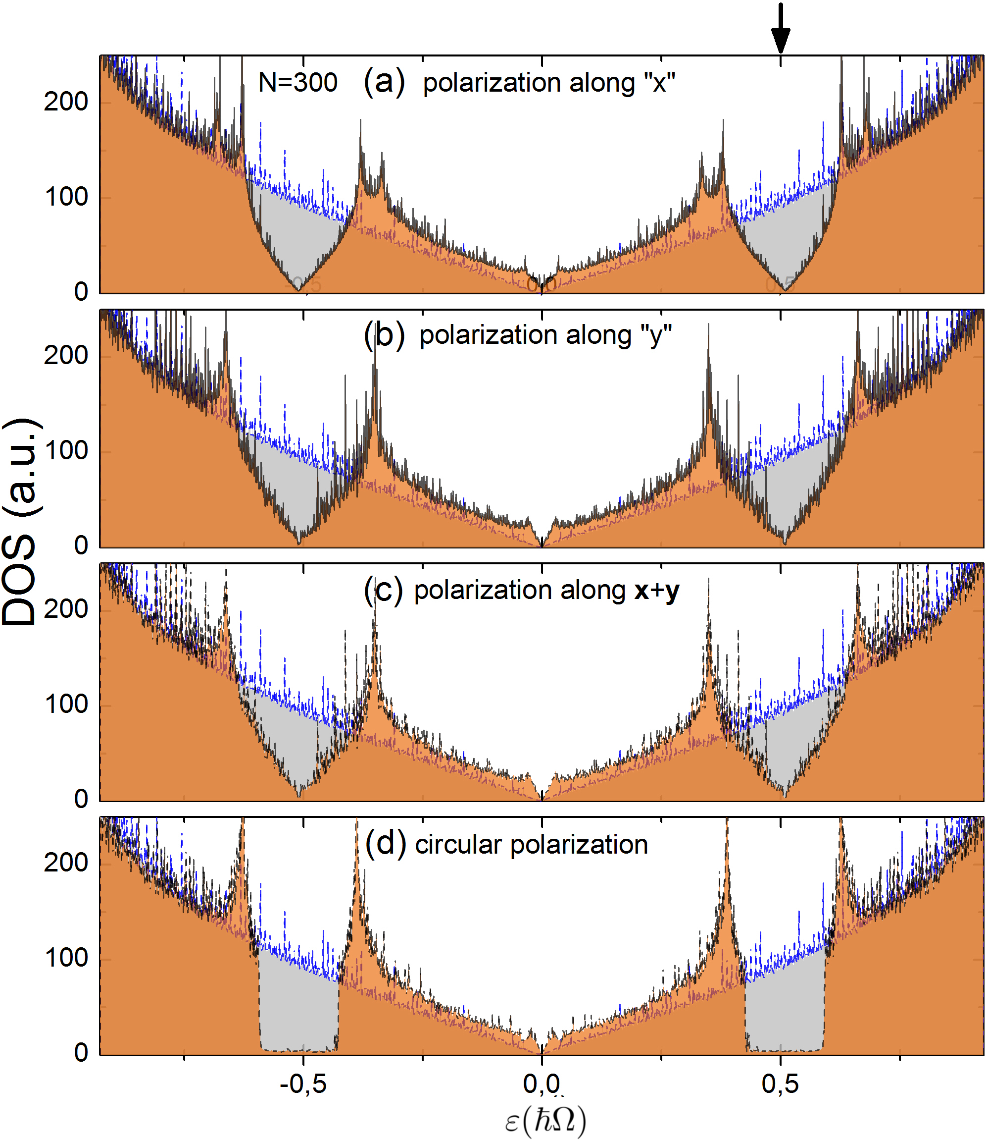
Figure 8: (Color online) Average density of states for an armchair graphene nanoribbon with $N=300$ in the presence of linearly polarized radiation along the $x$ (a), $y$ (b) and $\mathbf{x+y}$ (c) directions. Circular polarization is shown in panel d. For a better visualization of the bulk limit a large value of $\Omega$ was taken, $\hbar\Omega=\gamma_{0}=2.7\,\mathrm{eV}$.

3.1 Bulk limit

Now that the origin of the features observed in figures 4 and 7 has been clarified, we turn to the issue of how the bulk limit is achieved. For a ribbon with a high number of modes, a very large number of crossings in the Floquet spectrum become “accumulated” in the neighbourhood of $\pm n\hbar\Omega/2$. Once the separation between these features becomes small enough, the depletions merge and the system is insensitive to the particular direction of the (linear) polarization. To illustrate the emergence of the bulk limit we refer to figure 8 showing the DOS for an armchair ribbon with $N=300$. Linear polarization along the $x$, $y$ and $\bf{x}+\bf{y}$ directions, respectively, are considered in panels $a$,$b$ and $c$, while circular polarization is shown in panel $d$. To account for a large number of bands around the region $\hbar\Omega/2$, we increase significantly the frequency and power of the laser to get a flavor of the bulk effects while keeping the dimension of the Floquet space treatable. A direct observation of panels $a$ to $c$ shows that the sharp features observed in figures 4 and 6 for linearly polarized laser are now averaged in such a way that the same DOS is obtained for any direction of the laser. On the other hand, qualitative differences between linear and circular polarization become evident in this limit, where one can see that a strong gap appears in the last case.

4 Conclusions

We have presented a detailed account of a simulation scheme for assessing the electrical properties (average conductance and density of states) of laser-illuminated graphene nanoribbons. The scheme is based on the application of Floquet theory to a realistic Hamiltonian which allows the simulation of system sizes beyond the scope of the usual k.p approximation. The usefulness of this scheme is illustrated on nanoribbons under different polarizations (linear and circular). A simple analysis allowed us to rationalize the emergence of the bulk 2d limit.

References

References

- [1] Geim A K 2009 Science 324 1934; Geim A K and Novoselov K S 2007 Nat. Mat. 6 183.
- [2] Castro Neto A H, Guinea F, Peres N M R, Novoselov K S and Geim A K 2009 Rev. Mod. Phys. 81 109.
- [3] Dubois S M M., Zanolli Z, Declerck X and Charlier J C 2009 Eur. Phys. J. B 72 1; Charlier J C, Blase X and Roche S 2007 Rev. Mod. Phys. 79 677; A. Cresti et al. 2008 Nano Research 1 361.
- [4] Bonaccorso F, Sun Z, Hasan T and Ferrari A C 2010 Nat. Photon. 4 611.
- [5] Xia F, Mueller T, Lin Y M, Valdes-Garcia A and Avouris P 2009 Nat. Nano. 4 839.
- [6] Karch J, Drexler C, Olbrich P, Fehrenbacher M, Hirmer M, Glazov M M, Tarasenko S A, Ivchenko E L, Birkner B, Eroms J, Weiss D, Yakimova R, Lara-Avila S, Kubatkin S, Ostler M, Seyller T and Ganichev S D 2011 Phys. Rev. Lett. 107 276601.
- [7] Jorio A, Saito R, Dresselhaus M and Dresselhaus G 2012 Raman spectroscopy of graphene-related systems (Weinheim: Wiley).
- [8] Gabor N M, Song J C W, Ma Q, Nair N L, Taychatanapat T, Watanabe K, Taniguchi T, Levitov L S and Jarillo-Herrero P 2011 Science 334 648.
- [9] Koppens F H L, Chang D E and García de Abajo F J 2011 Nano Lett. 11 3370.
- [10] Chen J, Badioli M, Alonso-Gonzalez P, Thongrattanasiri S, Huth F, Osmond J, Spasenovic M, Centeno A, Pesquera A, Godignon P, Zurutuza Elorza A, Camara N, García de Abajo F J, Hillenbrand R and Koppens F H L 2012 Nature advance online publication
- [11] Foa Torres L E F and Roche S 2006 Phys. Rev. Lett. 97 076804; Foa Torres L E F, Avriller R and Roche S 2008 Phys. Rev. B 78 035412.
- [12] Lazzeri M and Mauri F 2006 Phys. Rev. Lett. 97 266407.
- [13] Pisana S, Lazzeri M, Casiraghi C, Novoselov K S, Geim A K, Ferrari A C and Mauri F 2007 Nat. Mater. 6 198.
- [14] Syzranov S V, Fistul M V and Efetov K B 2008 Phys. Rev. B 78 045407.
- [15] Oka T and Aoki H 2009 Phys. Rev. B 79 081406.
- [16] Calvo H L, Pastawski H M, Roche S and Foa Torres L E F 2011 Appl. Phys. Lett. 98 232103.
- [17] Zhou Y and Wu M W 2011 Phys. Rev. B 83 245436.
- [18] Savel ev S E and Alexandrov A S 2011 Phys. Rev. B 84 035428.
- [19] Busl M, Platero G and Jauho A P 2012 Phys. Rev. B 85 155449.
- [20] Kibis O V 2010 Phys. Rev. B 81 165433.
- [21] Iurov A, Gumbs G, Roslyak O and Huang D 2012 J. Phys.: Condens. Matter 24 015303.
- [22] Liu J T, Su F H, Wang H and Deng X H 2012 New J. Phys. 14 013012.
- [23] San-Jose P, Prada E, Schomerus H and Kohler S 2012 Appl. Phys. Lett. 101 153506.
- [24] Lindner N H, Refael G, Galitski V 2011 Nat Phys 7 490.
- [25] Kitagawa T, Oka T, Brataas A, Fu L and Demler E 2011 Phys. Rev. B 84 235108.
- [26] Gu Z, Fertig H A, Arovas D P and Auerbach A 2011 Phys. Rev. Lett. 107 216601.
- [27] Suarez Morell E, and Foa Torres L E F, to appear in Phys. Rev. B. 2012.
- [28] Cayssol J, Dóra B, Simon F and Moessner R 2012 arXiv:1211.5623v2 [cond-mat.mes-hall].
- [29] Rudner M S, Lindner N H, Berg E and Levin M arxiv:1212.3324[cond-mat.mes.hall].
- [30] Crespi A and Corrielli G, Valle G D, Osellame R and Longhi S 2013 New J. Phys. 15 013012.
- [31] Rechtsman M C, Zeuner J M, Plotnik Y, Lumer Y, Nolte S, Segev, M, and Szameit A arxiv:1212.3146[physics.optics].
- [32] Abergel D S L and Chakraborty T 2009 Appl. Phys. Lett. 95 062107.
- [33] Calvo H L, Piskunow P M P, Roche S, and Foa Torres L E F 2012 Appl. Phys. Lett. 101 253506.
- [34] Pastawski H M and Medina E 2001 Rev. Mex. Fis. 47S1 1.
- [35] Peierls R E 1933 Z. Phys. 80 763.
- [36] Shirley J H 1965 Phys. Rev. 138 B979; Sambe H 1973 Phys. Rev. A 7 2203.
- [37] Kohler S, Lehmann J and Hänggi P 2005 Phys. Rep. 406 379.
- [38] Martinez D F 2003 J. Phys. A 36 9827.
- [39] Foa Torres L E F 2005 Phys. Rev. B 72 245339.
- [40] Levstein P. R., Pastawski H. M. and D’Amato J. L. 1990 J. Phys.: Condens. Matter 2 1781.
- [41] Stefanucci G, Kurth S, Rubio A and Gross E K U 2008 Phys. Rev. B 77(7) 075339.