A Concise Formula for Generalized Two-Qubit Hilbert-Schmidt Separability Probabilities

Abstract

We report major advances in the research program initiated in ”Moment-Based Evidence for Simple Rational-Valued Hilbert-Schmidt Generic $2\times 2$ Separability Probabilities” (J. Phys. A, 45, 095305 [2012]). A highly succinct separability probability function $P(\alpha)$ is put forth, yielding for generic (9-dimensional) two-rebit systems, $P(\frac{1}{2})=\frac{29}{64}$, (15-dimensional) two-qubit systems, $P(1)=\frac{8}{33}$ and (27-dimensional) two-quater(nionic)bit systems, $P(2)=\frac{26}{323}$. This particular form of $P(\alpha)$ was obtained by Qing-Hu Hou by applying Zeilberger’s algorithm (”creative telescoping”) to a fully equivalent–but considerably more complicated–expression containing six ${}_{7}F_{6}$ hypergeometric functions (all with argument $\frac{27}{64}=(\frac{3}{4})^{3}$). That hypergeometric form itself had been obtained using systematic, high-accuracy probability-distribution-reconstruction computations. These employed 7,501 determinantal moments of partially transposed $4\times 4$ density matrices, parameterized by $\alpha=\frac{1}{2},1,\frac{3}{2},2,\ldots,32$. From these computations, exact rational-valued separability probabilities were discernible. The (integral/half-integral) sequences of 32 rational values, then, served as input to the Mathematica FindSequenceFunction command, from which the initially obtained hypergeometric form of $P(\alpha)$ emerged.

I Introduction

Our study will be devoted to addressing the fundamental quantum-information-theoretic problem, first apparently, explicitly discussed by Życzkowski, Horodecki, Lewenstein and Sanpera (ZHSL) Życzkowski et al. (1998) in their highly-cited 1998 paper, ”Volume of the set of separable states” Życzkowski et al. (1998). They gave ”three main reasons of importance”–philosophical, practical and physical–for examining such problems (cf. Singh et al. ).) Specifically, we will address the problem raised in Życzkowski et al. (1998) of what proportion (that is, ”separability probability”) of quantum states are separable/disentangled Werner (1989). We endow the (generalized two-qubit) states, to which we confine our attention here, with the Hilbert-Schmidt (Euclidean/flat) metric and its accompanying measure Życzkowski and Sommers (2003); Bengtsson and Życzkowski (2006). It is certainly also of interest to study the problem posed by ZHSL in alternative–but perhaps even more challenging analytically–settings, in particular that of the Bures (minimal monotone) metric/measure Sommers and Życzkowski (2003); Bengtsson and Życzkowski (2006); Slater (2000, 2005a); Osipov et al. (2010); Ye (2009); Slater (2012).

We do report an apparent resolution of the ZHSL separability-probability problem in the generalized two-qubit Hilbert-Schmidt context, in terms of the titular ”concise formula”, which we will denote by $P(\alpha)$. Though we still lack a fully rigorous argument for its validity, the formula strongly appears to fulfill the indicated role, while manifesting important mathematical (random matrix theory Dumitriu et al. (2007); Bhosale et al. (2012),…) and physical (quantum entanglement Bhosale et al. (2012); Życzkowski et al. (1998); Bengtsson and Życzkowski (2006)) properties. Thus, we have

$$P(\alpha)=\Sigma_{i=0}^{\infty}f(\alpha+i),$$ (1)

where

$$f(\alpha)=P(\alpha)-P(\alpha+1)=\frac{q(\alpha)2^{-4\alpha-6}\Gamma{(3\alpha+\frac{5}{2})}\Gamma{(5\alpha+2})}{3\Gamma{(\alpha+1)}\Gamma{(2\alpha+3)}\Gamma{(5\alpha+\frac{13}{2})}},$$ (2)

and

$$q(\alpha)=185000\alpha^{5}+779750\alpha^{4}+1289125\alpha^{3}+1042015\alpha^{2}+410694\alpha+63000=$$ (3)

$$\alpha\bigg{(}5\alpha\Big{(}25\alpha\big{(}2\alpha(740\alpha+3119)+10313\big{)}+208403\Big{)}+410694\bigg{)}+63000.$$

A reader, equipped with any standard contemporary mathematical language programming package (Maple, Mathematica, Matlab,…), can readily verify that (to arbitrarily high-precision [hundreds/thousands of digits]), quite remarkably (but not yet formally proven mat ), $P(0)=1,P(\frac{1}{2})=\frac{29}{64},P(1)=\frac{8}{33}$ and $P(2)=\frac{26}{323}$ (Figs. 3 and fig:HouGraph). In terms of the physical implications of the formula, we find compelling evidence that $P(\alpha)$ yields the separability probability Życzkowski et al. (1998)–with respect to Hilbert-Schmidt measure–of generalized two-qubit states, where, in particular $\alpha=0,\frac{1}{2},1,2$ correspond to classical, rebit, qubit and quater(nionic)bit states, respectively.

We will indicate below the multistep procedure by which the particular concise form of $P(\alpha)$ presented above was obtained. This process depended upon, first, the derivation Slater and Dunkl (2012) of (hypergeometric-based) formulas for the moments of probability distributions over the determinants of partially transposed density matrices, followed by the estimation (using a certain Legendre-polynomial-based probability-distribution-reconstruction procedure Provost (2005)) from those moments of cumulative (over the separability interval) probabilities. Then, $\alpha$-parameterized sequences of these cumulative probabilities were analyzed to extract the underlying structure captured by $P(\alpha)$. This initially took a relatively complicated hypergeometric form (Fig. 3), from which the concise formula above was subsequently derived (Figs. 5 and 6) by Qing-Hu Hou using Zeilberger’s algorithm Zeilberger (1990).

I.1 Background

The underpinning, predecessor paper Slater and Dunkl (2012)–addressing the relatively long-standing $2\times 2$ separability probability question Życzkowski et al. (1998); Slater (2005a, 2002, 1999, 2000, b, 2007a, 2008, 2006, 2007b) (cf. Szarek (2005); Aubrun and Szarek (2006); Ye (2009))–consisted largely of two sets of analyses. The first set was concerned with establishing formulas for the bivariate determinantal product moments $\left\langle\left|\rho^{PT}\right|^{n}\left|\rho\right|^{k}\right\rangle,k,n=0,1,2,3,\ldots,$ with respect to Hilbert-Schmidt (Euclidean/flat) measure (Bengtsson and Życzkowski, 2006, sec. 14.3) Życzkowski and Sommers (2003), of generic (9-dimensional) two-rebit and (15-dimensional) two-qubit density matrices ($\rho$). Here $\rho^{PT}$ denotes the partial transpose of the $4\times 4$ density matrix $\rho$. Nonnegativity of the determinant $|\rho^{PT}|$ is both a necessary and sufficient condition for separability in this $2\times 2$ setting Augusiak et al. (2008).

In the second set of primary analyses in Slater and Dunkl (2012), the univariate determinantal moments $\left\langle\left|\rho^{PT}\right|^{n}\right\rangle$ and $\left\langle\left(|\rho^{PT}\right|\left|\rho\right|)^{n}\right\rangle$, induced using the bivariate formulas, served as input to a Legendre-polynomial-based probability distribution reconstruction algorithm of Provost (Provost, 2005, sec. 2) (cf. Pintarelli and Vericat (2011)). This yielded estimates of the desired separability probabilities. (The reconstructed probability distributions based on $|\rho^{PT}|$ are defined over the interval $|\rho^{PT}|\in[-\frac{1}{16},\frac{1}{256}]$, while the associated separability probabilities are the cumulative probabilities of these distributions over the nonnegative subinterval $|\rho^{PT}|\in[0,\frac{1}{256}]$. We note that for the fully mixed (classical) state, $|\rho^{PT}|=\frac{1}{256}$, while for a maximally entangled state, such as a Bell state, $|\rho^{PT}|=-\frac{1}{16}$, thus, delimiting the range of $|\rho^{PT}|$.)

A highly-intriguing aspect of the (not yet rigorously established) determinantal moment formulas obtained (by C. Dunkl) in (Slater and Dunkl, 2012, App.D.4) was that both the two-rebit ($\alpha=\frac{1}{2}$) and two-qubit ($\alpha=1$) cases could be encompassed by a single formula, with a Dyson-index-like parameter $\alpha$ Dumitriu and Edelman (2002) serving to distinguish the two cases. Additionally, the results of the formula for $\alpha=2$ and $n=1$ and 2 have recently been confirmed computationally by Dunkl using the ”Moore determinant” (quasideterminant) Moore (1922); Gelfand et al. (2005) of $4\times 4$ quaternionic density matrices. (However, tentative efforts of ours to verify the $\alpha=4$ [conjecturally, octonionic Liao et al. (2010), problematical] case, have not proved successful.)

When the probability-distribution-reconstruction algorithm Provost (2005) was applied in Slater and Dunkl (2012) to the two-rebit case ($\alpha=\frac{1}{2}$), employing the first 3,310 moments of $|\rho^{PT}|$, a (lower-bound) estimate that was 0.999955 times as large as $\frac{29}{64}\approx 0.453120$ was obtained (cf. (Slater, 2010, p. 6)).

Analogously, in the two-qubit case ($\alpha=1$), using 2,415 moments, an estimate that was 0.999997066 times as large as $\frac{8}{33}\approx 0.242424$ was derived. This constitutes an appealingly simple rational value that had previously been conjectured in a quite different (non-moment-based) form of analysis, in which ”separability functions” had been the main tool employed Slater (2007b). (Note, however, that the two-rebit separability probability conjecture of $\frac{8}{17}$, somewhat secondarily advanced in Slater (2007b), has now been discarded in favor of $\frac{29}{64}$.) Let us note, supportively, that in an extensive Monte Carlo analysis, Zhou, Chern, Fei and Joynt obtained an estimate for this two-qubit separability probability of $0.2424\pm 0.0002$ (Zhou et al., 2012, eq. (B7)). Additionally, in the very same context, Fonseca-Romero, Rincón and Viviescas report a compatible statistic of $24\%$ (Fonseca-Romero et al., 2012, sec. VIII).

Further, the determinantal moment formulas advanced in Slater and Dunkl (2012) were then applied with $\alpha$ set equal to 2. This appears–as the indicated recent (Moore determinant) computations of Dunkl show–to correspond to the generic 27-dimensional set of quaternionic density matrices Andai (2006); Adler (1995). Quite remarkably, a separability probability estimate, based on 2,325 moments, that was 0.999999987 times as large as $\frac{26}{323}\approx 0.0804954$ was found.

II Outline of Present Study

In the present study, we extend these three (individually-conducted) moment-based analyses in a more systematic, thorough manner, jointly embracing the sixty-four integral and half-integral values $\alpha=\frac{1}{2},1,\frac{3}{2},2,\ldots,32$. We do this by accelerating, for our specific purposes, the Mathematica probability-distribution-reconstruction program of Provost Provost (2005), in a number of ways. Most significantly, we make use of the three-term recurrence relations for the Legendre polynomials. Doing so obviates the need to compute each successive higher-degree Legendre polynomial ab initio.

In this manner, we were able to obtain–using exact computer arithmetic throughout–”generalized” separability probability estimates based on 7,501 moments for $\alpha=\frac{1}{2},1,\frac{3}{2},\ldots,32$. In Fig. 1 we plot the logarithms of the resultant sixty-four separability probability estimates (cf. (Slater and Dunkl, 2012, Fig. 8)), which fall close to the line $-0.9464181889\alpha$.

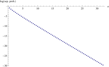
Figure 1: Logarithms of generalized separability probability estimates, based on 7,501 Hilbert-Schmidt moments of $|\rho^{PT}|$, as a function of the Dyson-index-like parameter $\alpha$

In Fig. 2 we show the residuals from this linear fit.

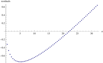
Figure 2: Residuals from linear fit to logarithms of generalized separability probability estimates

In Fig. 3 we present a hypergeometric-function-based formula, together with striking supporting evidence for it, that appears to succeed in uncovering the functional relation ($P(\alpha)$) underlying the entirely of these sixty-four generalized separability probabilities.

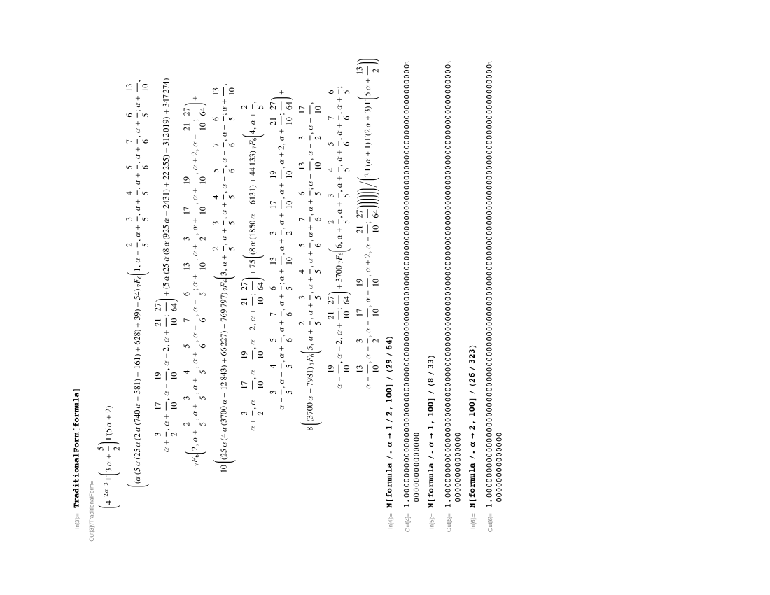
Figure 3: Hypergeometric formula $P(\alpha)$ for Hilbert-Schmidt generic $2\times 2$ generalized separability probabilities and evidence that it reproduces the basic three (real [$\alpha=\frac{1}{2}$], complex [$\alpha=1$] and quaternionic [$\alpha=2$]) conjectures of $\frac{29}{64},\frac{8}{33}$ and $\frac{26}{323}$

Further, in (6), and the immediately preceding text, we list a number of remarkable values yielded by this hypergeometric formula for values of $\alpha$ other than the basic sixty-four (half-integral and integral) values from which we have started.

Then, we are able to report–with the assistance of Qing-Hu Hou–a striking condensation of the lengthy expression presented in Fig. 3, that is, the titular ”concise formula” (eqs. (1)-(3)).

Some additional computational results of interest are presented in the Appendix.

III New Results

III.1 The three basic (rebit, qubit, quaterbit) conjectures revisited

III.1.1 $\alpha=\frac{1}{2}$–the two-rebit case

In Slater and Dunkl (2012), a lower-bound estimate of the two-rebit separability probability was obtained, with the use of the first 3,310 moments of $|\rho^{PT}|$. It was 0.999955 times as large as $\frac{29}{64}\approx 0.453120$. With the indicated use, now, of 7,501 moments, the figure increases to 0.999989567. This outcome, thus, fortifies our previous conjecture.

III.1.2 $\alpha=1$–the two-qubit case

In Slater and Dunkl (2012), a lower-bound estimate of the two-qubit separability probability was obtained, with the use of the first 2,415 moments of $|\rho^{PT}|$, that was 0.999997066 times as large as $\frac{8}{33}\approx 0.242424$ (cf. (Zhou et al., 2012, eq. (B7))). Employing 7,501 moments, this figure increases to 0.99999986.

III.1.3 $\alpha=2$–the quaternionic case

In Slater and Dunkl (2012), a lower-bound estimate of the (presumptive) quaternionic separability probability was obtained that was 0.999999987 times as large as $\frac{26}{323}\approx 0.0804954$, using the first 2,325 moments of $|\rho^{PT}|$. Based on 7,501 moments, this figure increases, quite remarkably still, to 0.999999999936.

III.2 Generalized separability probability hypergeometric formula

A principal motivation in undertaking the analyses reported here–in addition, to further scrutinizing the three specific conjectures reported in Slater and Dunkl (2012)–was to uncover the functional relation underlying the curve in Fig. 1 (and/or its original non-logarithmic counterpart).

Preliminarily, let us note that the zeroth-order approximation (being independent of the particular value of $\alpha$) provided by the Provost Legendre-polynomial-based probability-distribution-reconstruction algorithm is simply the uniform distribution over the interval $|\rho^{PT}|\in[-\frac{1}{16},\frac{1}{256}]$. The corresponding zeroth-order separability probability estimate is the cumulative probability of this distribution over the nonnegative subinterval $[0,\frac{1}{256}]$, that is, $\frac{1}{256}/(\frac{1}{16}+\frac{1}{256})=\frac{1}{17}\approx 0.0588235$. So, it certainly appears that speedier convergence (sec. III.1) of the algorithm occurs for separability probabilities, the true values of which are initially close to $\frac{1}{17}$ (such as $\frac{26}{323}\approx 0.0804954$ in the quaternionic case). Convergence also markedly increases as $\alpha$ increases.

It appeared, numerically, that the generalized separability probabilities for integral and half-integral values of $\alpha$ were rational values (not only $\frac{29}{64},\frac{8}{33},\frac{26}{323}$, for the three specific values $\alpha=\frac{1}{2},1,2$ of original focus). With various computational tools and search strategies based upon emerging mathematical properties, we were able to advance additional, seemingly plausible conjectures as to the exact values for $\alpha=3,4,\ldots,32$, as well. (We inserted many of our high-precision numerical estimates into the search box on the Wolfram Alpha website–which then indicated likely candidates for corresponding rational values.)

We fed this sequence of thirty-two conjectured rational numbers into the FindSequenceFunction command of Mathematica. (This command ”attempts to find a simple function that yields the sequence $a_{i}$ when given successive integer arguments,” but apparently can succeed with rational arguments, as well.) To our considerable satisfaction, this produced a generating formula (incorporating a diversity of hypergeometric functions of the ${}_{p}F_{p-1}$ type, $p=7,\ldots,11$, all with argument $z=\frac{27}{64}=(\frac{3}{4})^{3}$) for the sequence (cf. (Penson and Życzkowski, 2011, eq. (11))). (Let us note that $z^{-\frac{1}{2}}=\sqrt{\frac{64}{27}}$ is the ”residual entropy for square ice” (Finch, 2003, p. 412) (cf. (Krattenthaler and Rao, 2005, eqs.[(27), (28)). An analogous appearance of $\frac{27}{64}$ occurs in a hypergeometric [”Ramanujan-like”] summation for $\frac{16\pi^{2}}{3}$ of J. Guillera Guillera (2011). In a private communication, he remarked that the value $z=\frac{27}{64}$ appears to frequently occur in hypergeometric identities, and that this appears to have some modular or modular-like origin.). In fact, the Mathematica command succeeds using only the first twenty-eight conjectured rational numbers, but no fewer–so it seems fortunate, our computations were so extensive.)

However, the formula produced by the Mathematica command was quite cumbersome in nature (extending over several pages of output). With its use, nevertheless, we were able to convincingly generate rational values for half-integral $\alpha$ (including the two-rebit $\frac{29}{64}$ conjecture), also fitting our corresponding half-integral thirty-two numerical estimates exceedingly well. (Let us strongly emphasize that the hypergeometric-based formula was initially generated using only the integral values of $\alpha$. The process was fully reversible, and we could first employ the half-integral results to generate the formula–which then–seemingly perfectly fitted the integral values.)

At this point, for illustrative purposes, let us list the first ten half-integral and ten integral rational values (generalized separability probabilities), along with their approximate numerical values.

$$\begin{array}[]{cc}\begin{array}[]{cccc}\text{$\alpha$ =}&\frac{1}{2}&\frac{29}{64}&0.453125\\ \end{array}&\begin{array}[]{cccc}\text{$\alpha$ =}&1&\frac{8}{33}&0.242424\\ \end{array}\\ \begin{array}[]{cccc}\text{$\alpha$ =}&\frac{3}{2}&\frac{36061}{262144}&0.137562\\ \end{array}&\begin{array}[]{cccc}\text{$\alpha$ =}&2&\frac{26}{323}&0.0804954\\ \end{array}\\ \begin{array}[]{cccc}\text{$\alpha$ =}&\frac{5}{2}&\frac{51548569}{1073741824}&0.0480083\\ \end{array}&\begin{array}[]{cccc}\text{$\alpha$ =}&3&\frac{2999}{103385}&0.0290081\\ \end{array}\\ \begin{array}[]{cccc}\text{$\alpha$ =}&\frac{7}{2}&\frac{38911229297}{2199023255552}&0.0176948\\ \end{array}&\begin{array}[]{cccc}\text{$\alpha$ =}&4&\frac{44482}{4091349}&0.0108722\\ \end{array}\\ \begin{array}[]{cccc}\text{$\alpha$ =}&\frac{9}{2}&\frac{60515043681347}{9007199254740992}&0.00671852\\ \end{array}&\begin{array}[]{cccc}\text{$\alpha$ =}&5&\frac{89514}{21460999}&0.00417101\\ \end{array}\\ \begin{array}[]{cccc}\text{$\alpha$ =}&\frac{11}{2}&\frac{71925602948804923}{27670116110564327424}&0.0025994\\ \end{array}&\begin{array}[]{cccc}\text{$\alpha$ =}&6&\frac{179808469}{110638410169}&0.00162519\\ \end{array}\\ \begin{array}[]{cccc}\text{$\alpha$ =}&\frac{13}{2}&\frac{3387374833367307236269}{3324546003940230230441984}&0.0010189\\ \end{array}&\begin{array}[]{cccc}\text{$\alpha$ =}&7&\frac{191151001}{298529164591}&0.000640309\\ \end{array}\\ \begin{array}[]{cccc}\text{$\alpha$ =}&\frac{15}{2}&\frac{124792688228667229196729}{309485009821345068724781056}&0.000403227\\ \end{array}&\begin{array}[]{cccc}\text{$\alpha$ =}&8&\frac{1331199762}{5232880523393}&0.000254391\\ \end{array}\\ \begin{array}[]{cccc}\text{$\alpha$ =}&\frac{17}{2}&\frac{407557367133399293946182513}{2535301200456458802993406410752}&0.000160753\\ \end{array}&\begin{array}[]{cccc}\text{$\alpha$ =}&9&\frac{74195568677}{729345064647247}&0.000101729\\ \end{array}\\ \begin{array}[]{cccc}\text{$\alpha$ =}&\frac{19}{2}&\frac{1338799759394288468677657208071}{20769187434139310514121985316880384}&0.0000644609\\ \end{array}&\begin{array}[]{cccc}\text{$\alpha$ =}&10&\frac{730710456538}{17868447453498669}&0.0000408939\\ \end{array}\\ \end{array}$$ (4)

To simplify the cumbersome (several-page) output yielded by the Mathematica FindSequenceFunction command, we employed certain of the ”contiguous rules” for hypergeometric functions listed by C. Krattenthaler in his package HYP Krattenthaler (1995) (cf. Bytev et al. (2010)). Multiple applications of the rules C14 and C18 there, together with certain gamma function simplifications suggested by C. Dunkl, led to the rather more compact formula displayed in Fig. 3. This formula incorporates a six-member family ($k=1,\ldots,6$) of ${}_{7}F_{6}$ hypergeometric functions, differing only in the first upper index $k$,

$$\,_{7}F_{6}\left(k,\alpha+\frac{2}{5},\alpha+\frac{3}{5},\alpha+\frac{4}{5},\alpha+\frac{5}{6},\alpha+\frac{7}{6},\alpha+\frac{6}{5};\alpha+\frac{13}{10},\alpha+\frac{3}{2},\alpha+\frac{17}{10},\alpha+\frac{19}{10},\alpha+2,\alpha+\frac{21}{10};\frac{27}{64}\right).$$ (5)

(The reader will note interesting sequences of upper and lower parameters (cf. Zudilin (2011)).) We are only able to, in general, evaluate the formula numerically, but then to arbitrarily high (hundreds, if not thousand-digit) precision, giving us strong confidence–despite the lack yet of a formal proof (cf. mat )–in the validity of the exact generalized separability probabilities ($\frac{29}{64},\frac{8}{33},\frac{26}{323}$, …), that we advance.

III.2.1 Additional interesting values yielded by the hypergeometric formula

Let us now apply the formula (Fig. 3) to values of $\alpha$ other than the initial sixty-four studied. For $\alpha=0$, the formula yields–as would be expected–the ”classical separability probability” of 1. Further, proceeding in a purely formal manner (since there appears to be no corresponding genuine probability distribution over $[-\frac{1}{16},\frac{1}{256}]$), for the negative value $\alpha=-\frac{1}{2}$, the formula yields $\frac{2}{3}$. For $\alpha=-\frac{1}{4}$, it gives -2. Remarkably still, for $\alpha=\frac{1}{4}$, the result is clearly (to one thousand decimal places) equal to $2-\frac{34}{21\text{agm}\left(1,\sqrt{2}\right)}=2-\frac{17\Gamma\left(\frac{1}{4}\right)^{2}}{21\sqrt{2}\pi^{3/2}}\approx 0.6486993992$, where the arithmetic-geometric mean of 1 and $\sqrt{2}$ is indicated. (The reciprocal of this mean is Gauss’s constant.) For $\alpha=\frac{3}{4}$, the result equals $2-\frac{9689\Gamma\left(\frac{3}{4}\right)}{4420\sqrt{\pi}\Gamma\left(\frac{5}{4}\right)}\approx 0.3279684732$, while for $\alpha=-\frac{3}{4}$, we have $\frac{128}{21\text{agm}\left(1,\sqrt{2}\right)}+2=2+\frac{32\sqrt{2}\Gamma\left(\frac{1}{4}\right)^{2}}{21\pi^{3/2}}\approx 7.087249321$. For $\alpha=\frac{2}{3}$, the outcome is $2-\frac{288927\Gamma\left(\frac{1}{3}\right)^{3}}{344080\pi^{2}}\approx 0.36424897456$. Results are presented in the table

$$\left(\begin{array}[]{ccc}\alpha&P(\alpha)&\text{value}\\ -\frac{3}{4}&2+\frac{32\sqrt{2}\Gamma\left(\frac{1}{4}\right)^{2}}{21\pi^{3/2}}&7.08725\\ -\frac{2}{3}&2-\frac{8\pi}{\sqrt{3}\Gamma\left(\frac{1}{3}\right)^{3}}&1.24527\\ -\frac{1}{2}&\frac{2}{3}&0.666667\\ -\frac{1}{3}&2+\frac{3\Gamma\left(\frac{1}{3}\right)^{3}}{4\pi^{2}}&3.461\\ -\frac{1}{4}&2&2\\ \frac{1}{4}&2-\frac{17\Gamma\left(\frac{1}{4}\right)^{2}}{21\sqrt{2}\pi^{3/2}}&0.648699\\ \frac{1}{3}&2-\frac{459\sqrt{3}\pi}{91\Gamma\left(\frac{1}{3}\right)^{3}}&0.572443\\ \frac{2}{3}&2-\frac{288927\Gamma\left(\frac{1}{3}\right)^{3}}{344080\pi^{2}}&0.364249\\ \frac{3}{4}&2-\frac{9689\Gamma\left(\frac{3}{4}\right)}{4420\sqrt{\pi}\Gamma\left(\frac{5}{4}\right)}&0.327968\\ \end{array}\right).$$ (6)

(Let us note that the term $\frac{3\Gamma\left(\frac{1}{3}\right)^{3}}{4\pi^{2}}\approx 1.46099848$ present in the result for $\alpha=-\frac{1}{3}$ is ”Baxter’s four-coloring constant” for a triangular lattice (Finch, 2003, p. 413).) Also, for $\alpha=-1$, we have $\frac{2}{5}$. For $\alpha=-\frac{3}{2}$, the result is $\frac{2}{3}$.

IV Concise reformulation of ${}_{7}F_{6}$ hypergeometric expression (Fig. 3)

Figure 4: Generalized two-qubit separability probability function $P(\alpha)$, with $P(0)=1,P(\frac{1}{2})=\frac{29}{64},P(1)=\frac{8}{33},P(2)=\frac{26}{323}$ for generic classical four-level ($\alpha=0$), two-rebit ($\alpha=\frac{1}{2}$), two-qubit ($\alpha=1$) and two-quaterbit ($\alpha=2$) systems, respectively.

We had previously ourselves been unable to find an equivalent form of $P(\alpha)$ with fewer than six hypergeometric functions (Fig. 3). Qing-Hu Hou of the Center for Combinatorics of Nankai University, however, was able to obtain the remarkably succinct and clearly correct results (1)-(3)–which he communicated to us in a few e-mail messages. (Accompanying them were two Maple worksheets indicating his calculations [Figs. 5 and 6].) Hou, first, observed that the hypergeometric-based formula for $P(\alpha)$ could be expressed as an infinite summation. Letting $P_{l}(\alpha)$ be the $l$-th such summand, application of Zeilberger’s algorithm Zeilberger (1990) (a method for producing combinatorial identities, also known as ”creative telescoping”) yielded that

$$P_{l}(\alpha)-P_{l}(\alpha+1)=-P_{l+1}(\alpha)+P_{l}(\alpha).$$ (7)

(The package APCI–available at http://www.combinatorics.net.cn/homepage/hou/–was employed. In a different quantum-information context, Datta employed the algorithm to ascertain that no closed form exists for a certain series, ”retarding” the evaluation of the ”ratio of the negativity of random pure states to the maximal negativity for Haar-distributed states of $n$ qubits” (Datta, 2010, App. A, Table I).) Summing over $l$ from 0 to $\infty$, Hou found that

$$P(\alpha)-P(\alpha+1)=P_{0}(\alpha).$$ (8)

Letting $f(\alpha)=P_{0}(\alpha)$, the concise summation formula (1) is obtained. (C. Krattenthaler indicated [Krattenthaler, private communication] that these results might equally well be derived without recourse to Zeilberger’s algorithm. Also, a referee expressed puzzlement at the peculiar [redundant] form of eq. (7). This appears to be an artifact arising from the particular manner in which the algorithm is applied in the proving of hypergeometric identities.)

Figure 5: First Maple worksheet of Hou used in deriving concise form of hypergeometric formula (Fig. 3)

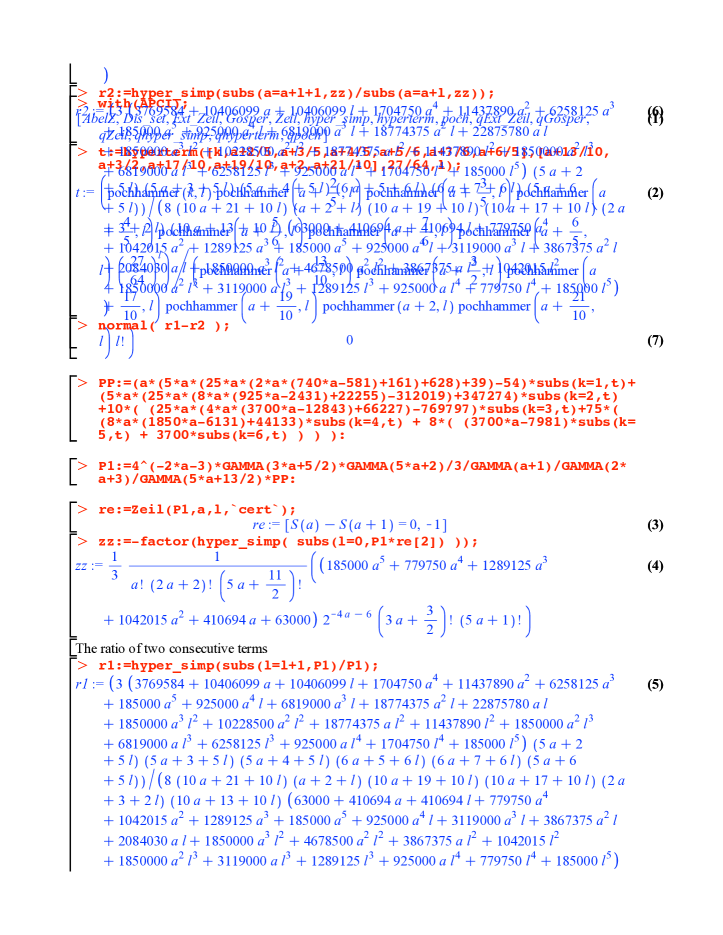
Figure 6: Second Maple worksheet of Hou used in deriving concise form of hypergeometric formula (Fig. 3)

We certainly need to indicate, however, that if we do explicitly perform the infinite summation indicated in (1), then we revert to a (”nonconcise”) form of $P(\alpha)$, again containing six hypergeometric functions. Further, it appears that we can only evaluate (1) numerically–but then easily to hundreds and even thousands of digits of precision–giving us extremely high confidence in the specific rational-valued Hilbert-Schmidt separability probabilities advanced.

V Concluding Remarks

There remain the important problems of formally verifying the formulas for $P(\alpha)$ (as well as the underlying determinantal moment formulas for $|\rho^{PT}|$, …, in Slater and Dunkl (2012), employed in the probability-distribution reconstruction process), and achieving a better understanding of what these results convey regarding the geometry of quantum states Bengtsson and Życzkowski (2006); Avron et al. (2007); Avron and Kenneth (2009). Further, questions of the asymptotic behavior of the formula ($\alpha\rightarrow\infty$) and of possible Bures metric Sommers and Życzkowski (2003); Bengtsson and Życzkowski (2006); Slater (2005a, 2002, 2000) counterparts to it, are under investigation Slater (2012).

We are presently engaged in attempting to determine further properties–in addition to the cumulative (separability) probabilities over $[0,\frac{1}{256}]$ obtained from the titular concise formula (eq. (1)-(3))–of the probability distributions of $|\rho^{PT}|$ over $[-\frac{1}{16},\frac{1}{256}]$, as a function of the Dyson-index-like parameter $\alpha$. As one such finding, it appears that the $y$-intercept (at which $|\rho^{PT}|=0$, that is, the separability-entanglement boundary) in the presumed quaternionic case ($\alpha=2$) is $\frac{7425}{34}=\frac{3^{3}\times 5^{2}\times 11}{2\times 17}\approx 218.382$ Slater . (The Legendre-polynomial-based probability-distribution reconstruction algorithm of Provost Provost (2005) yielded an estimate 0.99999999742 times as large as $\frac{7425}{34}$, when implemented with 10,000 moments. Based also on 10,000 moments–but with inferior convergence properties–the two-qubit [$\alpha=1$] and two-rebit [$\alpha=\frac{1}{2}$] $y$-intercepts were estimated as 389.995 (conjecturally equal to $390=2\cdot 3\cdot 5\cdot 13$) and 502.964, respectively Slater .)

The foundational paper of Życzkowski, Horodecki, Sanpera and Lewenstein,”Volume of the set of separable states” Życzkowski et al. (1998) (cf. Singh et al. ), did ask for volumes, not specifically probabilities. At least, for the two-rebit, two-qubit and two-quaterbit cases, $\alpha=\frac{1}{2},1$ and $2$, we can readily, using the Hilbert-Schmidt volume formulas of Andai (Andai, 2006, Thms. 1-3) (cf. Życzkowski and Sommers (2003); Bengtsson and Życzkowski (2006)), convert the corresponding separability probabilities to the separable volumes $\frac{29\pi^{4}}{61931520}=\frac{29\pi^{4}}{2^{16}\cdot 3^{3}\cdot 5\cdot 7}$, $\frac{\pi^{6}}{449513064000}=\frac{\pi^{6}}{2^{6}\cdot 3^{6}\cdot 5^{3}\cdot 7^{2}\cdot 11^{2}\cdot 13}$ and $\frac{\pi^{12}}{3914156909371803494400000}=\frac{\pi^{12}}{2^{14}\cdot 3^{10}\cdot 5^{5}\cdot 7^{3}\cdot 11^{2}\cdot 13\cdot 17^{2}\cdot 19^{2}\cdot 23}$, respectively. The determination of separable volumes–as opposed to probabilities–for other values of $\alpha$ than these fundamental three appears to be rather problematical, however.

Let us also note the relevance of the study of Szarek, Bengtsson and Życzkowski Szarek et al. (2006), in which they show that the convex set of separable mixed states of the $2\times 2$ system is a body of constant height. Theorem 2 of that paper, in conjunction with the results here, allows one, it would seem, to immediately deduce that the separability probabilities of the generic minimally-degenerate/boundary 8-, 14-, and 26-dimensional two-rebit, two-qubit, and two-quaterbit states are one-half (that is, $\frac{29}{128},\frac{4}{33}$ and $\frac{13}{323}$) the separability probabilities of their generic non-degenerate counterparts.

VI Appendix–Exact values of derivatives of $P(\alpha)$

VI.1 Succeeding deriviatives at $\alpha=0$

The first derivative of $P(\alpha)$ evaluated at (the classical case) $\alpha=0$ is -2, while the second derivative is $40-20\zeta{(2)}=40-\frac{10\pi^{2}}{3}\approx 7.10132$. (The third derivative was computed as -43.7454236566749417600.)

VI.2 First derivatives at $\alpha=1,2\ldots$, et al

The first derivative of $P(\alpha)$ at $\alpha=-\frac{1}{2}$ is $-\frac{80}{3}$ and at $\alpha=\frac{1}{2}$ is $\frac{1}{384}(917-984\log(2))\approx 0.611831$, and -2 at $\alpha=0$, as previously mentioned. We have also been able to determine rational values of $P(\alpha)$ for $\alpha=1,2,\ldots,97$. We list the first seven of these. (The Mathematica command FindSequenceFunction, however, did not succeed in this instance in generating an underlying function for this sequence of 97 rational numbers–although, of course, one can be directly obtained from our explicit form of $P(\alpha)$.)

$$\left(\begin{array}[]{ccc}\alpha&P^{\prime}(\alpha)\\ 1&-\frac{130577}{457380}\approx-0.285489\\ 2&-\frac{3177826243}{37595998440}\approx-0.0845257\\ 3&-\frac{3598754002551529}{124409677632540300}\approx-0.0289266\\ 4&-\frac{943222153906869801499}{89625168823088671652880}\approx-0.0105241\\ 5&-\frac{7745868905935978063871447}{1956135029605259737354520400}\approx-0.00395978\\ 6&-\frac{163704960709243940550573265691777}{107569184582725029279135417408286275}\approx-0.00152186\\ 7&-\frac{124555275071579876642057723808475761407}{209867628485254931732709294271962333917400}\approx-0.000593494\\ \end{array}\right).$$ (9)