Weighted Sum Rate Maximization for
Downlink OFDMA with Subcarrier-pair based
Opportunistic DF Relaying

Abstract

This paper addresses a weighted sum rate (WSR) maximization problem for downlink OFDMA aided by a decode-and-forward (DF) relay under a total power constraint. A novel subcarrier-pair based opportunistic DF relaying protocol is proposed. Specifically, user message bits are transmitted in two time slots. A subcarrier in the first slot can be paired with a subcarrier in the second slot for the DF relay-aided transmission to a user. In particular, the source and the relay can transmit simultaneously to implement beamforming at the subcarrier in the second slot. Each unpaired subcarrier in either the first or second slot is used for the source’s direct transmission to a user. A benchmark protocol, same as the proposed one except that the transmit beamforming is not used for the relay-aided transmission, is also considered. For each protocol, a polynomial-complexity algorithm is developed to find at least an approximately optimum resource allocation (RA), by using continuous relaxation, the dual method, and Hungarian algorithm. Instrumental to the algorithm design is an elegant definition of optimization variables, motivated by the idea of regarding the unpaired subcarriers as virtual subcarrier pairs in the direct transmission mode. The effectiveness of the RA algorithm and the impact of relay position and total power on the protocols’ performance are illustrated by numerical experiments. It is shown that for each protocol, it is more likely to pair subcarriers for relay-aided transmission when the total power is low and the relay lies in the middle between the source and user region. The proposed protocol always leads to a maximum WSR equal to or greater than that for the benchmark one, and the performance gain of using the proposed one is significant especially when the relay is in close proximity to the source and the total power is low. Theoretical analysis is presented to interpret these observations.

I Introduction

Orthogonal frequency division multiple access (OFDMA) has been widely recognized as one of the dominant wireless technologies for high data-rate transmission. One of the main reasons behind this fact is that spectral efficiency of the OFDM(A) systems can be improved significantly by proper resource allocation (RA) when transmitter channel state information (CSI) is available [1, 2, 3]. The incorporation of decode-and-forward (DF) and amplify-and-forward (AF) relaying into OFDM(A) systems through subcarrier-pair based protocols and associated RA have lately been under intensive investigation [4, 5, 6, 7, 8, 9, 10, 11, 12, 13, 14, 15, 16, 17, 18, 19, 20, 21, 22, 23, 24, 25, 26, 27, 28, 29]. This class of protocols share the following features. User message bits are transmitted during two consecutive equal-duration time slots. In the first slot, the source broadcasts OFDM symbols, so does the relay in the second slot. The source might also emit OFDM symbols during the second slot as will be elaborated later. A subcarrier in the first slot can be paired with a subcarrier in the second slot for transmitting message bits with DF/AF relaying, referred to as the relay-aided transmission mode hereafter.

In this paper, we focus on RA for downlink OFDMA with subcarrier-pair based DF relaying (there also exist works on RA for OFDMA systems using bidirectional relaying [4]). The subcarrier-pair based AF relaying has been studied in [5, 6, 7, 8]. Note that the subcarrier-by-subcarrier based pairing may not be sufficient for DF relaying, since the information from a set of subcarriers in the first time slot can be decoded and re-encoded jointly and then forwarded through a different set of subcarriers in the second time slot [8, 12]. Nevertheless, the subcarrier-pair based DF relaying has attracted much research interest due to simplicity or practical reasons [12, 9, 10, 11, 13, 14, 15, 16, 17, 18, 19, 20, 21, 22, 23, 24, 25, 26, 27, 28, 29].

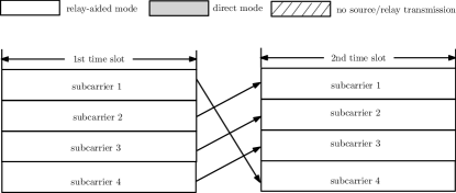
(a) when the S-D link is unavailable [12, 9, 10, 11].

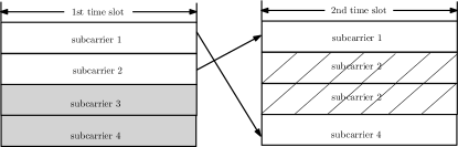
(b) when the S-D link is available but the source does not transmit in the second slot [13, 14, 15, 16, 17, 18, 19, 20].

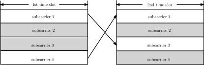
(c) when the S-D link is available and the source transmits in the second slot [21, 22, 23, 24, 25, 26, 27, 28, 29].

Figure 1: Illustration of the subcarrier-pair based DF relaying protocols for OFDM(A)-based systems, where every arrow indicates that the two associated subcarriers are paired for the relay-aided transmission.

When the source-to-destination (S-D) link is unavailable (i.e., the destination lies outside the source’s radio coverage), RA problems for OFDM systems using subcarrier-pair based DF protocols have been addressed in [9, 10, 11, 12]. In these works, every subcarrier in the first time slot is paired with a subcarrier in the second time slot for the relay-aided transmission, as illustrated in Fig. 1.a. To maximize sum rate under a total power constraint, ordered subcarrier pairing has been proven to be the optimum, i.e., the strongest source-to-relay subcarrier should be paired with the strongest relay-to-destination subcarrier, and so on.

The works in [13, 14, 15, 16, 17, 18, 19, 20, 21, 22, 23, 24, 25, 26, 27, 28, 29] have considered the case where the S-D link is available. When only the relay emits OFDM symbols in the second time slot, opportunistic relaying (sometimes termed as selection relaying) was studied in [13, 14, 15, 16, 17, 18, 19, 20]. Specifically, a subcarrier in the first time slot can either be paired with a subcarrier in the second slot for the relay-aided transmission, or used directly for the S-D transmission without the relay’s assistance, referred to as the direct transmission mode hereafter. It is very important to note that when some subcarriers in the first slot are used in the direct transmission mode, some subcarriers in the second slot will not be used as illustrated in Fig. 1.b, which leads to a waste of precious spectrum resource.

To address the above issue, improved protocols which allow the source to emit OFDM symbols in the second slot were proposed and studied in [21, 22, 23, 25, 26, 24, 27, 28, 29]. The improved protocols are the same as those considered in [13, 14, 15, 16, 17, 18], except that the source can also make direct S-D transmission at every unpaired subcarrier in the second slot, as illustrated in Fig. 1.c. Note that the improved protocols do not really improve the way that DF relaying is implemented over a subcarrier pair, but rather let the source utilize the unpaired subcarriers in the second slot for direct transmission to avoid the waste of spectrum resource. In [24, 27, 29], the subcarrier pairing and power allocation are jointly optimized for point-to-point OFDM systems. As for OFDMA systems, RA problems considering the joint optimization of power allocation, subcarrier assignment to users and selection of multiple relays for transmit beamforming in the second slot are addressed in [25, 26]. In these works, a priori and CSI-independent subcarrier pairing is considered, i.e., a subcarrier in the first slot is always paired with the same subcarrier in the second slot if the relay-aided mode is used. The optimization of subcarrier pairing and assignment to users is addressed in [28] with a graph based approach. It is a complicated RA problem to jointly optimize subcarrier pairing and mode selection with power allocation and subcarrier assignment to users.

Compared with the above existing works, this paper makes the following contributions:

• A novel subcarrier-pair based opportunistic DF protocol is proposed for downlink OFDMA aided by a DF relay. This protocol further makes improvement over those previously studied in the literature [21, 22, 23, 24, 25, 26, 27, 28, 29], by allowing the source and the relay to implement transmit beamforming at a subcarrier in the second time slot for the relay-aided transmission. Note that the protocols studied in [25, 26] considered the selection of multiple DF relays (excluding the source) for transmit beamforming in the second slot, while the proposed protocol considers the joint source-relay transmit beamforming. A benchmark protocol, which is the same as the proposed one except for the relay-aided transmission mode, is also considered. Note that the proposed protocol truly improves the implementation of DF relaying over a subcarrier pair with transmit beamforming, which is not the case for the benchmark protocol.

• The weighted sum rate (WSR) maximized RA problem is addressed for both the proposed and benchmark protocols under a total power constraint for the whole system. First, it is shown that the proposed protocol leads to a maximum WSR not smaller than that for the benchmark one. Then, an algorithm is developed for each protocol to find at least an approximately optimum RA with a WSR very close to the maximum WSR. Instrumental to the elegance of the RA algorithm is a definition of appropriate indicator variables, making it possible to cast a subproblem related to the joint optimization of transmission-mode selection, subcarrier pairing and assignment to users into an standard assignment problem that can be solved efficiently by Hungarian algorithm.

The rest of this paper is organized as follows. In the next section, the system and transmission protocols are described. The theoretical analysis is made to compare the maximum WSRs of the two protocols in Section III. After that, the RA algorithm is developed in Section IV. Numerical experiments are shown to illustrate the effectiveness of the RA algorithm and study the impact of relay position and total power on the protocols’ performance in Section V. Finally, some conclusions are drawn.

Notations: A letter in bold, e.g. $\bf x$, represents a set. $\mathcal{C}(x)=\frac{1}{2}\log_{2}(1+x)$.

II Protocols and WSR maximization problem

II-A The transmission system and protocols

Consider the downlink OFDMA transmission from a source to $U$ users (user $u=1,\dots,U$) aided by a DF relay. The source, relay and every user are each equipped with a single antenna, and the channel between every two of them is frequency selective. The source and the relay are synchronized so that they can simultaneously emit OFDM symbols using $K$ subcarriers and with sufficiently long cyclic prefix to eliminate inter-symbol interference.

The novel transmission protocol is half-duplex, i.e., user message bits are transmitted in two consecutive equal-duration time slots, during which all channels are assumed to keep unchanged. During the first slot, only the source broadcasts $N$ OFDM symbols. Both the relay and all users receive these symbols. After proper processing explained later, the source and relay simultaneously broadcast $N$ OFDM symbols, and the users receive them during the second slot.

Due to the OFDMA, each subcarrier is dedicated to transmitting a single user’s message exclusively. A subcarrier in the first slot can be paired with a subcarrier in the second slot for the relay-aided mode transmission to a user. Each unpaired subcarrier in either the first or second slot is used by the source for the direct mode transmission to a user.

To simplify description, we use subcarriers $k$ and $l$ to denote the $k$th and $l$th subcarriers used during the first and second slots, respectively ($k,l=1,\cdots,K$). We define the source transmission powers for subcarrier $k$ in the first slot and subcarrier $l$ in the second slot as $P_{{\rm s},k,1}$ and $P_{{\rm s},l,2}$, respectively. The relay transmission power for subcarrier $l$ is $P_{{\rm r},l,2}$. The complex amplitude gains at subcarrier $k$ for the source-to-relay, source-to-$u$ and relay-to-$u$ channels are $h_{\mathrm{sr},k}$, $h_{\mathrm{s}u,k}$ and $h_{\mathrm{r}u,k}$, respectively. The two transmission modes for the novel protocol are elaborated as follows:

II-A1 The relay-aided transmission mode

Suppose subcarrier $k$ is paired with subcarrier $l$ for the relay-aided mode transmission to user $u$. In such a case, we refer to the two subcarriers collectively as the subcarrier pair $(k,l)$. A block of message bits are first encoded into a code word of complex symbols $\{\theta(n)|n=1,\cdots,N\}$ with $E(|\theta(n)|^{2})=1$, $\forall\;n$. In the first slot, the source broadcasts the codeword over subcarrier $k$ as illustrated in Figure 2.a. At the relay and user $u$, the $n$th baseband signals received through subcarrier $k$ are

$$y_{{\rm r},k}(n)=\sqrt{P_{{\rm s},k,1}}h_{\mathrm{sr},k}\theta(n)+z_{{\rm r},k}(n),n=1,\cdots,N,$$ (1)

and

$$y_{u,k,1}(n)=\sqrt{P_{{\rm s},k,1}}h_{\mathrm{s}u,k}\theta(n)+z_{u,k,1}(n),n=1,\cdots,N,$$ (2)

respectively, where $z_{{\rm r},k}(n)$ and $z_{u,k,1}(n)$ are both additive white Gaussian noise (AWGN) with power $\sigma^{2}$. The signal-to-noise ratio (SNR) at the relay is $P_{{\rm s},k,1}G_{\mathrm{sr},k}$ where $G_{\mathrm{sr},k}=\frac{|h_{\mathrm{sr},k}|^{2}}{\sigma^{2}}$. At the end of the first time slot, the relay decodes the message bits from $\{y_{{\rm r},k}(n)|n=1,\cdots,N\}$ and then reencodes those bits into the same codeword as the source did.

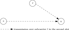
Figure 2: The relay-aided transmission mode over the subcarrier pair $(k,l)$ to user $u$.

In the second time slot, the source and relay broadcast the codewords $\{\theta(n)e^{-j\angle h_{\mathrm{s}u,l}}|\forall\;n\}$ and $\{\theta(n)e^{-j\angle h_{\mathrm{r}u,l}}|\forall\;n\}$ through subcarrier $l$, respectively, where $\angle h_{\mathrm{s}u,l}$ and $\angle h_{\mathrm{r}u,l}$ represent the phase of $h_{\mathrm{s}u,l}$ and $h_{\mathrm{r}u,l}$, respectively. This means that the source and relay implement transmit beamforming to emit the codeword through subcarrier $l$ as illustrated in Figure 2.b. Note that the source and relay need to know the phase of $h_{\mathrm{s}u,l}$ and $h_{\mathrm{r}u,l}$, respectively. At user $u$, the $n$th baseband signal received through subcarrier $l$ is

$$y_{u,l,2}(n)=\big{(}\sqrt{P_{{\rm s},l,2}}|h_{\mathrm{s}u,l}|+\sqrt{P_{{\rm r},l,2}}|h_{\mathrm{r}u,l}|\big{)}\theta(n)+z_{u,l,2}(n),$$ (3)

where $z_{u,l,2}(n)$ is the AWGN with power $\sigma^{2}$.

Finally, user $u$ decodes the message bits from all signals received during the two slots. These signals can be grouped into $N$ vectors, the $n$th of which is

$${\bf y}(n) =\left[\begin{array}[]{c}y_{u,k,1}(n)\\ y_{u,l,2}(n)\end{array}\right]$$ (6)

$$=\left[\begin{array}[]{c}\sqrt{P_{{\rm s},k,1}}h_{\mathrm{s}u,k}\\ \sqrt{P_{{\rm s},l,2}}|h_{\mathrm{s}u,l}|+\sqrt{P_{{\rm r},l,2}}|h_{\mathrm{r}u,l}|\end{array}\right]\theta(n)+{\bf z}(n),$$ (9)

where ${\bf z}(n)=[z_{u,k,1}(n),z_{u,l,2}(n)]^{T}$. Note that the transmission in effect makes $N$ uses of a discrete memoryless single-input-two-output channel specified by (6), with the $n$th input and output being $\theta(n)$ and ${\bf y}(n)$, respectively. To achieve the maximum reliable transmission rate, maximum ratio combining should be used [30], i.e., user $u$ first turns every ${\bf y}(n)$ into a decision variable

$$c(n)=(\sqrt{P_{{\rm s},k,1}}h_{\mathrm{s}u,k})^{*}y_{u,k,1}(n)+$$

$$\hskip 56.9055pt\big{(}\sqrt{P_{{\rm s},l,2}}|h_{\mathrm{s}u,l}|+\sqrt{P_{{\rm r},l,2}}|h_{\mathrm{r}u,l}|\big{)}^{*}y_{u,l,2}(n),$$ (10)

and then decodes the message from $\{c(n)|\forall\;n\}$. It can readily be derived that the SNR for this decoding is

$${\gamma}_{klu}(P_{{\rm s},k,1},P_{{\rm s},l,2},P_{{\rm r},l,2})=G_{\mathrm{s}u,k}P_{{\rm s},k,1}+$$

$$\hskip 56.9055pt\big{(}\sqrt{G_{\mathrm{s}u,l}P_{{\rm s},l,2}}+\sqrt{G_{\mathrm{r}u,l}P_{{\rm r},l,2}}\big{)}^{2},$$ (11)

where $G_{\mathrm{s}u,k}=\frac{|h_{\mathrm{s}u,k}|^{2}}{\sigma^{2}}$ and $G_{\mathrm{r}u,l}=\frac{|h_{\mathrm{r}u,l}|^{2}}{\sigma^{2}}$.

To ensure both the relay and user $u$ can reliably decode the message bits, the maximum number of message bits that can be transmitted is $2N\mathcal{C}(G_{\mathrm{sr},k}P_{{\rm s},k,1})$ and $2N\mathcal{C}({\gamma}_{klu}(P_{{\rm s},k,1},P_{{\rm s},l,2},P_{{\rm r},l,2}))$, respectively. This means that the maximum transmission rate over the subcarrier pair $(k,l)$ in the relay-aided mode to user $u$ is equal to $\mathcal{C}(\min\{G_{\mathrm{sr},k}P_{{\rm s},k,1},{\gamma}_{klu}(P_{{\rm s},k,1},P_{{\rm s},l,2},P_{{\rm r},l,2})\})$ bits/OFDM-symbol (bpos).

II-A2 The direct transmission mode

Suppose subcarrier $k$ (respectively, subcarrier $l$) is unpaired with any subcarrier in the second (respectively, first) slot, and is used for direct mode transmission to user $u$. The source first encodes message bits into a codeword of $N$ symbols, which are then broadcast through subcarrier $k$ (respectively, subcarrier $l$. In such a case, the relay keeps silent at subcarrier $l$ in the second slot, i.e. $P_{{\rm r},l,2}=0$.). User $u$ decodes the message bits from the signals received through subcarrier $k$ (respectively, subcarrier $l$). The maximum rate through subcarrier $k$ (respectively, subcarrier $l$) in the direct transmission mode is $\mathcal{C}(P_{{\rm s},k,1}G_{\mathrm{s}u,k})$ (respectively, $\mathcal{C}(P_{{\rm s},l,2}G_{\mathrm{s}u,l})$) bpos.

A benchmark protocol is also considered. This protocol is the same as the novel protocol except for the relay-aided transmission mode. Specifically, the relay-aided mode is the same as that widely studied in the literature [13, 14, 15, 16, 17, 18, 21, 22, 23, 24, 25, 26, 27], i.e., the source does not transmit at subcarrier $l$ during the second slot, if subcarriers $k$ and $l$ are paired for the relay-aided transmission to user $u$. In such a case, the maximum rate for the relay-aided transmission over that subcarrier pair to user $u$ is equal to $\mathcal{C}(\min\{G_{\mathrm{sr},k}P_{{\rm s},k,1},G_{\mathrm{s}u,k}P_{{\rm s},k,1}+G_{\mathrm{r}u,l}P_{{\rm r},l,2}\})$ bpos. It is important to note that, the benchmark protocol is a special case of the novel protocol, since it is equivalent to the novel protocol with the constraint that $P_{{\rm s},l,2}=0$ if subcarrier $l$ is paired with a subcarrier in the first slot for the relay-aided mode transmission.

II-B The WSR maximization problem

We assume there exists a central controller which knows precisely the CSI $\{G_{\mathrm{sr},k},G_{\mathrm{s}u,k},G_{\mathrm{r}u,k}|\forall\;k\}$. Before the data transmission, the controller needs to find the optimum subcarrier and power assignment, i.e., which subcarriers should be paired for the relay-aided mode and which should be in the direct mode, how these subcarriers should be assigned to the users, as well as the source/relay power allocation to maximize the WSR of all users for the adopted transmission protocol (which can be either the novel or benchmark protocol), when the total power consumption is not higher than a prescribed value $P_{\rm t}$. Then, the controller can inform the source and the relay about the optimum subcarrier and power assignment to be adopted for data transmission.

III Theoretical analysis

It can be shown that the proposed protocol leads to a maximum WSR greater than or equal to that for the benchmark protocol. To this end, suppose the optimum subcarrier assignment and power allocation has been found for the benchmark protocol. By using the proposed protocol with the same subcarrier assignment and power allocation, the same WSR can be achieved. Obviously, the maximum WSR for the proposed protocol is greater than or equal to that WSR, namely the maximum WSR for the benchmark protocol.

In Section III-A, we assume subcarriers $k$ and $l$ are paired for the relay-aided mode transmission to user $u$, and a sum power $P$ is used for this pair. We focus on computing the maximum rate and optimum power allocation of this pair for both protocols. Using these results, theoretical analysis will be made in Section III-B to show when the maximum WSR for the proposed protocol is strictly greater than that for the benchmark one, and the RA algorithm will be developed in Section IV. Moreover, this analysis plays an important role to interpret the numerical experiments shown in Section V to illustrate the impact of the relay’s position on the benefit of using the proposed protocol.

III-A Rate maximization for the pair in the relay-aided mode

III-A1 Analysis for the proposed protocol

To facilitate derivation, define $\Delta_{u,k}=G_{\mathrm{sr},k}-G_{\mathrm{s}u,k}$ and $G_{u,l}=G_{\mathrm{s}u,l}+G_{\mathrm{r}u,l}$. To maximize the rate, the optimum $P_{{\rm s},k,1}$, $P_{{\rm s},l,2}$ and $P_{{\rm r},l,2}$ are the optimum solution for

$$\max_{P_{{\rm s},k,1},P_{{\rm s},l,2},P_{{\rm r},l,2}} \hskip 5.69046pt\min\{G_{\mathrm{sr},k}P_{{\rm s},k,1},{\gamma}_{klu}(P_{{\rm s},k,1},P_{{\rm s},l,2},P_{{\rm r},l,2})\}$$

$${\rm s.t.} \hskip 5.69046ptP_{{\rm s},k,1}+P_{{\rm s},l,2}+P_{{\rm r},l,2}=P,$$ (12)

$$\hskip 5.69046ptP_{{\rm s},k,1}\geq 0,P_{{\rm s},l,2}\geq 0,P_{{\rm r},l,2}\geq 0.$$

By using the Cauchy-Schwartz inequality, it can be shown that

$${\gamma}_{klu}(P_{{\rm s},k,1},P_{{\rm s},l,2},P_{{\rm r},l,2})\leq G_{\mathrm{s}u,k}P_{{\rm s},k,1}+G_{u,l}P_{2},$$ (13)

where $P_{2}=P_{{\rm s},l,2}+P_{{\rm r},l,2}$ and the inequality is tight when $P_{{\rm s},l,2}=\frac{G_{\mathrm{s}u,l}}{G_{u,l}}P_{2}$ and $P_{{\rm r},l,2}=\frac{G_{\mathrm{r}u,l}}{G_{u,l}}P_{2}$. Now, the optimum solution for (12) can be found by first solving

$$\max_{P_{{\rm s},k,1},P_{2}} \hskip 5.69046pt\min\{G_{\mathrm{sr},k}P_{{\rm s},k,1},G_{\mathrm{s}u,k}P_{{\rm s},k,1}+G_{u,l}P_{2}\}$$ (14)

$${\rm s.t.} \hskip 5.69046ptP_{{\rm s},k,1}+P_{2}=P,P_{{\rm s},k,1}\geq 0,P_{2}\geq 0$$

for the optimum $P_{{\rm s},k,1}$ and $P_{2}$, and then using that $P_{2}$ to compute the optimum $P_{{\rm s},l,2}$ and $P_{{\rm r},l,2}$ according to the formulas that tighten the inequality (13). Problem (14) can be solved intuitively as follows. First, the two lines

$$\mathcal{L}_{0} =\{(x,y_{0}(x))|x\in[0,P],y_{0}(x)=G_{\mathrm{sr},k}x\}$$

$$\mathcal{L}_{1} =\{(x,y_{1}(x))|x\in[0,P],y_{1}(x)=G_{\mathrm{s}u,k}x+G_{u,l}(P-x)\}$$

can be plot over the two-dimensional plane of coordinates $(x,y)$ in Fig. 3. It can be seen that three different cases are possible, each corresponding to a specific orientation of the two lines. The coordinates of points $A$, $B$, $C$ and $D$ in the figure are shown in Table I. The optimum $P_{{\rm s},k,1}$ and objective value for (14) (which are also for (12)) are equal to the $x$ and $y$ coordinates of the points $A$, $B$ and $D$ for the three cases in Fig. 3, respectively. From this fact, it can easily be seen that the optimum $P_{{\rm s},k,1}$, $P_{{\rm s},l,2}$ and $P_{{\rm r},l,2}$ for (12) are

$$P_{{\rm s},k,1}=\left\{\begin{array}[]{ll}\frac{G_{u,l}}{\Delta_{u,k}+G_{u,l}}P&{\rm if\;}\min\{G_{\mathrm{sr},k},G_{u,l}\}>G_{\mathrm{s}u,k},\\ P&{\rm if\;}\min\{G_{\mathrm{sr},k},G_{u,l}\}\leq G_{\mathrm{s}u,k},\end{array}\right.$$ (17)

$$P_{{\rm s},l,2}=\left\{\begin{array}[]{ll}\frac{G_{\mathrm{s}u,l}}{G_{u,l}}\frac{\Delta_{u,k}}{(\Delta_{u,k}+G_{u,l})}P&{\rm if\;}\min\{G_{\mathrm{sr},k},G_{u,l}\}>G_{\mathrm{s}u,k},\\ 0&{\rm if\;}\min\{G_{\mathrm{sr},k},G_{u,l}\}\leq G_{\mathrm{s}u,k},\end{array}\right.$$ (20)

and

$$P_{{\rm r},l,2}=\left\{\begin{array}[]{ll}\frac{G_{\mathrm{r}u,l}}{G_{u,l}}\frac{\Delta_{u,k}}{(\Delta_{u,k}+G_{u,l})}P&{\rm if\;}\min\{G_{\mathrm{sr},k},G_{u,l}\}>G_{\mathrm{s}u,k},\\ 0&{\rm if\;}\min\{G_{\mathrm{sr},k},G_{u,l}\}\leq G_{\mathrm{s}u,k}.\end{array}\right.$$ (23)

The maximum rate associated with the above optimum solution is equal to $\mathcal{C}(G^{\rm n}_{klu}P)$ with

$$G^{\rm n}_{klu}=\left\{\begin{array}[]{ll}\frac{G_{\mathrm{sr},k}G_{u,l}}{\Delta_{u,k}+G_{u,l}}&{\rm if\;}\min\{G_{\mathrm{sr},k},G_{u,l}\}>G_{\mathrm{s}u,k},\\ \min\{G_{\mathrm{sr},k},G_{\mathrm{s}u,k}\}&{\rm if\;}\min\{G_{\mathrm{sr},k},G_{u,l}\}\leq G_{\mathrm{s}u,k}.\end{array}\right.$$ (26)

Figure 3: Illustration of the two lines $\mathcal{L}_{0}$ and $\mathcal{L}_{1}$ in three different cases.

TABLE I: Coordinates of A, B, C and D in Figure 3.

	$A$	$B$	$C$	$D$
$x$	$P$	$P$	$0$	$\frac{G_{u,l}}{\Delta_{u,k}+G_{u,l}}P$
$y$	$G_{\mathrm{sr},k}P$	$G_{\mathrm{s}u,k}P$	$G_{u,l}P$	$\frac{G_{\mathrm{sr},k}G_{u,l}}{\Delta_{u,k}+G_{u,l}}P$

III-A2 Analysis for the benchmark protocol

In this case, $P_{{\rm s},l,2}=0$ and the optimum $P_{{\rm s},k,1}$ and $P_{{\rm r},l,2}$ for maximizing the rate are the optimum solution for

$$\max_{P_{{\rm s},k,1},P_{{\rm r},l,2}} \hskip 5.69046pt\min\{P_{{\rm s},k,1}G_{\mathrm{sr},k},P_{{\rm s},k,1}G_{\mathrm{s}u,k}+P_{{\rm r},l,2}G_{\mathrm{r}u,l}\}$$ (27)

$${\rm s.t.} \hskip 5.69046ptP_{{\rm s},k,1}+P_{{\rm r},l,2}=P,P_{{\rm s},k,1}\geq 0,P_{{\rm r},l,2}\geq 0,$$

which can also be solved by the intuitive method as described above. It can be shown that the optimum $P_{{\rm s},k,1}$ and $P_{{\rm r},l,2}$ are

$$P_{{\rm s},k,1}=\left\{\begin{array}[]{ll}\frac{G_{\mathrm{r}u,l}}{\Delta_{u,k}+G_{\mathrm{r}u,l}}P&{\rm if\;}\min\{G_{\mathrm{sr},k},G_{\mathrm{r}u,l}\}>G_{\mathrm{s}u,k},\\ P&{\rm if\;}\min\{G_{\mathrm{sr},k},G_{\mathrm{r}u,l}\}\leq G_{\mathrm{s}u,k},\end{array}\right.$$ (30)

and

$$P_{{\rm r},l,2}=\left\{\begin{array}[]{ll}\frac{\Delta_{u,k}}{\Delta_{u,k}+G_{\mathrm{r}u,l}}P&{\rm if\;}\min\{G_{\mathrm{sr},k},G_{\mathrm{r}u,l}\}>G_{\mathrm{s}u,k},\\ 0&{\rm if\;}\min\{G_{\mathrm{sr},k},G_{\mathrm{r}u,l}\}\leq G_{\mathrm{s}u,k},\end{array}\right.$$ (33)

and the maximum rate associated with the above optimum solution is equal to $\mathcal{C}(G^{\rm b}_{klu}P)$ with

$$G^{\rm b}_{klu}=\left\{\begin{array}[]{ll}\frac{G_{\mathrm{sr},k}G_{\mathrm{r}u,l}}{\Delta_{u,k}+G_{\mathrm{r}u,l}}&{\rm if\;}\min\{G_{\mathrm{sr},k},G_{\mathrm{r}u,l}\}>G_{\mathrm{s}u,k},\\ \min\{G_{\mathrm{sr},k},G_{\mathrm{s}u,k}\}&{\rm if\;}\min\{G_{\mathrm{sr},k},G_{\mathrm{r}u,l}\}\leq G_{\mathrm{s}u,k}.\end{array}\right.$$ (36)

III-B Comparison of the two protocols

To compare the maximum WSR for the two protocols, it is necessary to first compare $G^{\rm n}_{klu}$ and $G^{\rm b}_{klu}$. When $G_{\mathrm{s}u,k}\geq\min\{G_{\mathrm{sr},k},G_{\mathrm{r}u,l}\}$, $G^{\rm b}_{klu}=\min\{G_{\mathrm{sr},k},G_{\mathrm{s}u,k}\}$. If $\min\{G_{\mathrm{sr},k},G_{u,l}\}\leq G_{\mathrm{s}u,k}$, $G^{\rm n}_{klu}=\min\{G_{\mathrm{sr},k},G_{\mathrm{s}u,k}\}=G^{\rm b}_{klu}$ follows. If $\min\{G_{\mathrm{sr},k},G_{u,l}\}>G_{\mathrm{s}u,k}$, it can be seen that $G^{\rm n}_{klu}P$ and $G_{\mathrm{s}u,k}P$ correspond to the $y$-coordinates of points $D$ and $B$ in Figure 3.c, respectively, and therefore $G^{\rm n}_{klu}>G_{\mathrm{s}u,k}$ since $D$ is higher than $B$. This means that $G^{\rm n}_{klu}\geq G^{\rm b}_{klu}$ always holds when $G_{\mathrm{s}u,k}\geq\min\{G_{\mathrm{sr},k},G_{\mathrm{r}u,l}\}$.

When $\min\{G_{\mathrm{sr},k},G_{\mathrm{r}u,l}\}>G_{\mathrm{s}u,k}$, $G^{\rm n}_{klu}$ and $G^{\rm b}_{klu}$ can be compared through a visualization method as follows. Specifically, we plot the lines $\mathcal{L}_{0}$, $\mathcal{L}_{1}$ and

$$\mathcal{L}_{2}=\{(x,y_{2}(x))| x\in[0,P],$$ (37)

$$y_{2}(x)=G_{\mathrm{s}u,k}x+G_{\mathrm{r}u,l}(P-x)\}$$

in Fig. 4. The coordinates of points $A$ and $B$ are the same as given in Tab. I, and those of points $C_{1}$, $C_{2}$, $D_{1}$ and $D_{2}$ are given in Tab. II. Most interestingly, $G^{\rm n}_{klu}P$ and $G^{\rm b}_{klu}P$ are equal to the $y$-coordinate of $D_{1}$ and $D_{2}$, respectively, and $C_{1}$ is above $C_{2}$ since $G_{u,l}\geq G_{\mathrm{r}u,l}$. In particular, the following points should be noted:

• $G^{\rm n}_{klu}>G^{\rm b}_{klu}$ holds because $D_{1}$ is above $D_{2}$.

• when $G_{\mathrm{sr},k}$ increases (meaning that point $A$ is elevated), $G^{\rm n}_{klu}-G^{\rm b}_{klu}$ increases (since the difference of the $y$-coordinate of points $D_{1}$ and $D_{2}$ is increased).

• when $G_{\mathrm{r}u,l}$ increases (meaning that points $C_{1}$ and $C_{2}$ are both elevated), $G^{\rm n}_{klu}-G^{\rm b}_{klu}$ reduces, because

  $$G^{\rm n}_{klu}-G^{\rm b}_{klu}=\frac{\Delta_{u,k}G_{\mathrm{s}u,l}G_{\mathrm{sr},k}}{(\Delta_{u,k}+G_{\mathrm{s}u,l}+G_{\mathrm{r}u,l})(\Delta_{u,k}+G_{\mathrm{r}u,l})},$$

  is a decreasing function of $G_{\mathrm{r}u,l}$.

Figure 4: Illustration of $G^{\rm b}_{klu}$ and $G^{\rm n}_{klu}$ when $\min\{G_{\mathrm{sr},k},G_{\mathrm{r}u,l}\}>G_{\mathrm{s}u,k}$.

TABLE II: Coordinates of $C_{1}$, $C_{2}$, $D_{1}$ and $D_{2}$ in Fig. 4.

	$C_{1}$	$C_{2}$	$D_{1}$	$D_{2}$
$x$	$0$	$0$	$\frac{G_{u,l}}{\Delta_{u,k}+G_{u,l}}P$	$\frac{G_{\mathrm{r}u,l}}{\Delta_{u,k}+G_{\mathrm{r}u,l}}P$
$y$	$G_{u,l}P$	$G_{\mathrm{r}u,l}P$	$G^{\rm n}_{klu}P$	$G^{\rm b}_{klu}P$

The above analysis indicates that $G^{\rm n}_{klu}\geq G^{\rm b}_{klu}$ always holds, and $G^{\rm n}_{klu}-G^{\rm b}_{klu}$ increases when either $G_{\mathrm{sr},k}$ increases or $G_{\mathrm{r}u,l}$ reduces, if $\min\{G_{\mathrm{sr},k},G_{\mathrm{r}u,l}\}>G_{\mathrm{s}u,k}$.

Using the above results, we now show that the proposed protocol leads to a strictly higher maximum WSR than the benchmark protocol, if there exist at least two subcarriers that must be paired for the relay-aided transmission for the benchmark protocol to maximize the WSR. To this end, collect the subcarrier pairs that must be used by the benchmark protocol to maximize the WSR in the set $\Phi$, and $\forall\;(k,l)\in\Phi$, denote $u_{kl}$ and $P_{u_{kl}}$ as the user which should use this subcarrier pair and the sum power that should be assigned to this pair. The rate contributed by this pair must be equal to $\mathcal{C}(G_{klu_{kl}}^{\rm b}P_{u_{kl}})$ as shown earlier. In such a case, $\min\{G_{\mathrm{sr},k},G_{\mathrm{r}u_{kl},l}\}>G_{\mathrm{s}u_{kl},k}$ must be satisfied, because otherwise simply using subcarriers $k$ and $l$ separately in the direct mode can lead to a higher sum rate. Suppose the proposed protocol is now used with a suboptimum RA which adopts the same subcarrier assignment as the optimum RA for the benchmark protocol. For every subcarrier in the direct mode, this RA uses the same source power allocation as the optimum value for the benchmark protocol, and $\forall\;(k,l)\in\Phi$, this RA uses $P_{u_{kl}}$ as the sum power for the subcarrier pair $(k,l)$. The maximum rate for this subcarrier pair is equal to $\mathcal{C}(G_{klu_{kl}}^{\rm n}P_{u_{kl}})$. Since $\min\{G_{\mathrm{sr},k},G_{\mathrm{r}u_{kl},l}\}>G_{\mathrm{s}u_{kl},k}$ holds, $G_{klu_{kl}}^{\rm n}>G_{klu_{kl}}^{\rm b}$ follows from earlier analysis, and therefore $\mathcal{C}(G_{klu_{kl}}^{\rm n}P_{u_{kl}})>\mathcal{C}(G_{klu_{kl}}^{\rm b}P_{u_{kl}})$ must hold. This means that the proposed protocol has a strictly higher maximum WSR than the benchmark protocol.

IV RA Algorithm design

IV-A Formulation of the RA problem

To formulate the WSR maximization problem for the adopted protocol (which can be either the proposed or benchmark protocol), we define

$$G_{klu}=\left\{\begin{array}[]{ll}G^{\rm n}_{klu}&{\rm if\;the\;proposed\;protocol\;is\;adopted},\\ G^{\rm b}_{klu}&{\rm if\;the\;benchmark\;protocol\;is\;adopted}.\end{array}\right.$$ (40)

For any configuration of transmission-mode selection, subcarrier pairing and assignment to users used by the adopted protocol, suppose $m$ subcarrier pairs are assigned to the relay-aided transmission, then it is always possible to one-to-one associate the unpaired subcarriers in the two slots to form $K-m$ virtual subcarrier pairs, each allocated to possibly two different users for direct transmission separately. Motivated by this observation, the RA problem is formulated by defining the following variables:

• $t_{klu}\in\{0,1\}$ for any combination of $k,l,u$. $t_{klu}=1$ indicates that subcarrier $k$ is paired with subcarrier $l$ for the relay-aided transmission to user $u$.

• $P_{klu}\geq 0$ for any combination of $k,l,u$. When $t_{klu}=1$, $P_{klu}$ is used as the total power for the subcarrier pair $(k,l)$.

• $t_{klab}\in\{0,1\}$ for any combination of $k,l$ and $a,b\in{\bf U}$. $t_{klab}=1$ indicates that subcarrier $k$ is assigned in the direct transmission mode to user $a$ during the first slot, and so is subcarrier $l$ to user $b$ during the second slot.

• $\alpha_{klab}\geq 0$ and $\beta_{klab}\geq 0$ for any combination of $k,l,a,b$. When $t_{klab}=1$, $P_{{\rm s},k,1}$ and $P_{{\rm s},l,2}$ take the value of $\alpha_{klab}$ and $\beta_{klab}$, respectively.

Let us collect all indicator and power variables in the sets ${\bf I}$ and ${\bf P}$, respectively, and define ${\bf S}=\{{\bf I},{\bf P}\}$. Every feasible RA scheme can be described by an ${\bf S}$ satisfying simultaneously

$$t_{klu},t_{klab}\in\{0,1\},\forall\;k,l,u,a,b,$$ (41)

$$\sum_{l}\left(\sum_{u}t_{klu}+\sum_{a,b}t_{klab}\right)=1,\forall\;k,$$ (42)

$$\sum_{k}\left(\sum_{u}t_{klu}+\sum_{a,b}t_{klab}\right)=1,\forall\;l,$$ (43)

$$\sum_{k,l,u,a,b}\left(t_{klu}P_{klu}+t_{klab}(\alpha_{klab}+\beta_{klab})\right)\leq P_{\rm t},$$ (44)

$$P_{klu}\geq 0,\alpha_{klab}\geq 0,\beta_{klab}\geq 0,\forall\;k,l,u,a,b,$$ (45)

$$P_{klu}=0{\rm\;if\;}t_{klu}=0,\forall\;k,l,u,a,b,$$ (46)

$$\alpha_{klab}=0,\beta_{klab}=0{\rm\;if\;}t_{klab}=0,\forall\;k,l,u,a,b,$$ (47)

where (42) and (43) guarantee the OFDMA, i.e., every subcarrier is used exclusively for the transmission of message bits to a unique user. (44) and (45) ensure the total power constraint is satisfied. The constraints (46) and (47) are added to guarantee that every ${\bf S}$ is one-to-one mapped to a new variable for the change of variable (COV) proposed later to solve the RA problem.

Note that an ${\bf S}$ satisfying (41)-(47) indicates a unique feasible RA scheme for the adopted protocol. Viewed from the other way around, any feasible RA scheme can also be described by an ${\bf S}$ satisfying those constraints. Interestingly, the same feasible RA scheme might be described by multiple different ${\bf S}$ all satisfying these constraints. For instance, consider the scenario where there is only a single user $u$, and the RA scheme requiring messages to be transmitted in the direct mode, respectively, through subcarriers $k_{1}$ and $k_{2}$ during the first slot and subcarriers $l_{1}$ and $l_{2}$ during the second slot. This RA scheme can be described by using either an ${\bf S}$ with $t_{k_{1}l_{1}uu}=t_{k_{2}l_{2}uu}=1$ and $t_{k_{1}l_{2}uu}=t_{k_{2}l_{1}uu}=0$, or another ${\bf S}^{\prime}$ with $t_{k_{1}l_{2}uu}=t_{k_{2}l_{1}uu}=1$ and $t_{k_{1}l_{1}uu}=t_{k_{2}l_{2}uu}=0$.

Given a feasible ${\bf S}$, the maximum WSR for the adopted protocol is

$$f({\bf S})= \sum_{k,l,u,a,b}\big{(}t_{klu}w_{u}\mathcal{C}(G_{klu}P_{klu})+$$ (48)

$$\hskip 5.69046ptt_{klab}\big{(}w_{a}\mathcal{C}(G_{{\rm s}a,k}\alpha_{klab})+w_{b}\mathcal{C}(G_{{\rm s}b,l}\beta_{klab})\big{)},$$

where $w_{u}>0$ is the weight prescribed for user $u$. The WSR maximization problem is to solve

$${\rm(P1)\hskip 22.76228pt}\max_{{\bf S}}\hskip 7.11317ptf({\bf S})\hskip 7.11317pt{\rm s.t.}\hskip 7.11317pt\eqref{eq:first-constr}-\eqref{eq:last-constr}$$

for a globally optimum ${\bf S}$. We will develop an algorithm in the following subsections to find it, after which the optimum subcarrier assignment and source/relay power allocation can be computed according to the analysis in Section III-A.

IV-B The idea behind the RA algorithm design

Note that (P1) is a nonconvex program consisting of both continuous and binary variables, thus in general its duality gap is not zero. Similar nonconvex optimization problems for multicarrier systems exist in the literature [31, 32]. A possible approach to tackle them is to show their duality gaps approach zero when a sufficiently large number of subcarriers is used. This justifies the use of the dual method to find an asymptotically optimum solution.

Here, we use a continuous-relaxation based approach to find at least an approximately optimum ${\bf S}$ for (P1). Similar methods were also used in [33, 34] to compute asymptotic capacity regions. Specifically, all indicator variables are first relaxed to be continuous within $[0,1]$, after which we get a new problem

$${\rm(P2)\hskip 22.76228pt}\max_{{\bf S}} \hskip 7.11317ptf({\bf S})\hskip 7.11317pt$$

$${\rm s.t.} \hskip 7.11317ptt_{klu},t_{klab}\in[0,1],\forall\;k,l,u,a,b,$$ (49)

$$\hskip 7.11317pt\eqref{eq:second-constr}-\eqref{eq:last-constr},$$

as a relaxation of (P1). Define the feasible set of (P2) as $\bf{F}_{{\bf S}}$. Obviously, the feasible set of (P1) is a subset of $\bf{F}_{{\bf S}}$.

Then, we make the COV from ${\bf P}$ to ${\bf\widetilde{P}}=\{{\widetilde{P}_{klu}},{\widetilde{\alpha}_{klab}},\widetilde{\beta}_{klab}|\forall k,l,u,a,b\}$, where every ${\widetilde{P}_{klu}}$, ${\widetilde{\alpha}_{klab}}$ and $\widetilde{\beta}_{klab}$ satisfy, respectively,

$${\widetilde{P}_{klu}}=t_{klu}P_{klu},{\widetilde{\alpha}_{klab}}=t_{klab}\alpha_{klab},\widetilde{\beta}_{klab}=t_{klab}\beta_{klab}.$$ (50)

After the COV, we collect all variables into ${\bf X}=\{{\bf I},{\bf\widetilde{P}}\}$. It is important to note that an ${\bf S}\in\bf{F}_{{\bf S}}$ is one-to-one mapped to an ${\bf X}\in\bf{F}_{{\bf X}}$, where $\bf{F}_{{\bf X}}$ contains the set of all ${\bf X}$’s satisfying (49), (42)-(43), as well as

$$\sum_{k,l,u,a,b}\left({\widetilde{P}_{klu}}+{\widetilde{\alpha}_{klab}}+\widetilde{\beta}_{klab}\right)\leq P_{\rm t},$$ (51)

$${\widetilde{P}_{klu}}\geq 0,{\widetilde{\alpha}_{klab}}\geq 0,\widetilde{\beta}_{klab}\geq 0,\forall\;k,l,u,a,b,$$ (52)

$${\widetilde{P}_{klu}}=0{\rm\;if\;}t_{klu}=0,\forall\;k,l,u,a,b,$$ (53)

$${\widetilde{\alpha}_{klab}}=0,\widetilde{\beta}_{klab}=0{\rm\;if\;}t_{klab}=0,\forall\;k,l,u,a,b.$$ (54)

As a function of ${\bf X}\in\bf{F}_{{\bf X}}$, the WSR can be rewritten as

$$g({\bf X})= f({\bf S}({\bf X}))$$

$$= \sum_{k,l,u,a,b}\big{(}w_{u}\phi(t_{klu},{\widetilde{P}_{klu}},G_{klu})$$ (55)

$$+w_{a}\phi(t_{klab},{\widetilde{\alpha}_{klab}},G_{{\rm s}a,k})+w_{b}\phi(t_{klab},\widetilde{\beta}_{klab},G_{{\rm s}b,l})\big{)},$$

where ${\bf S}({\bf X})$ represents the ${\bf S}$ corresponding to the ${\bf X}\in\bf{F}_{{\bf X}}$ and

$$\phi(t,x,G)=\left\{\begin{array}[]{ll}t\,\mathcal{C}(G\,\frac{x}{t})&{\rm if\;}t>0,\\ 0&{\rm if\;}t=0.\\ \end{array}\right.$$ (58)

It can readily be shown that $\phi(t,x,G)$ with fixed $G$ is a continuous and concave function of $t\geq 0$ and $x$, because it is a perspective function of $\mathcal{C}(Gx)$ which is concave of $x$ (see pages $89-90$ for more details in [35]). Therefore, $g({\bf X})$ is a concave function of ${\bf X}\in\bf{F}_{{\bf X}}$.

After solving

$${\rm(P3)\hskip 22.76228pt}\max_{{\bf X}} \hskip 7.11317ptg({\bf X})$$

$${\rm s.t.} \hskip 7.11317pt\eqref{eq:new-firstconstr},\eqref{eq:second-constr}-\eqref{eq:third-constr},\eqref{eq:new-forthconstr}-\eqref{eq:new-lastconstr},$$

for its global optimum, the ${\bf S}$ corresponding to this global optimum is the optimum solution for (P2). In the following subsection, we will focus on solving the problem

$${\rm(P4)\hskip 22.76228pt}\max_{{\bf X}} \hskip 7.11317ptg({\bf X})$$

$${\rm s.t.} \hskip 7.11317pt\eqref{eq:new-firstconstr},\eqref{eq:second-constr}-\eqref{eq:third-constr},\eqref{eq:new-forthconstr}-\eqref{eq:new-fifthconstr},$$

which is a relaxation of (P3) by omitting (53) and (54). Obviously, $\bf{F}_{{\bf X}}$ is a subset of the feasible set of (P4). Most interestingly, (P4) is a convex program, which can be solved by highly-efficient convex-optimization techniques. Define the optimum objective value for (P1) and (P4) as $f^{\star}$ and $g^{\star}$, respectively. According to the relaxations we made,

$$g^{\star}\geq\max_{{\bf X}\in\bf{F}_{{\bf X}}}g({\bf X})=\max_{{\bf S}\in\bf{F}_{{\bf S}}}f({\bf S})\geq f^{\star}$$

follows. Define a global optimum for (P4) as ${\bf X}^{\star}$. If we can find an ${\bf X}^{\star}$ that satisfies (53) and (54), and contains binary indicator variables (i.e., $t_{klu},t_{klab}\in\{0,1\},\forall\;k,l,u,a,b$), then it can readily be shown that ${\bf S}({\bf X}^{\star})$ must be a global optimum for (P1).

In practice, it may be difficult to find precisely a global optimum ${\bf X}^{\star}$ for (P4) in general. For instance, existing convex-optimization techniques such as the interior-point method or the dual method all search for the global optimum in an iterative manner, and finally produce an approximately optimum solution with an objective value very close to the optimum value. Motivated by this fact, suppose a solution ${\bf X}^{\prime}$ which satisfies

1. (53) and (54) and all indicator variables in ${\bf X}^{\prime}$ are binary;

2. $g^{\star}-g({\bf X}^{\prime})$ is very small;

can be found for (P4), then ${\bf S}({\bf X}^{\prime})$ is feasible for (P1) and $f^{\star}-f({\bf S}({\bf X}^{\prime}))$ is also very small because

$$f^{\star}-f({\bf S}({\bf X}^{\prime}))\leq g^{\star}-g({\bf X}^{\prime}),$$

which means that ${\bf S}({\bf X}^{\prime})$ can be taken as an approximately optimum solution for (P1).

In the following subsection, we use the dual method to solve (P4). Specifically, the ellipsoid method is used to search for the dual optimum. This ellipsoid method is reduced to the bisection method to update upper and lower bounds for the dual optimum iteratively until convergence. In some cases, the global optimum for (P1) can be found, while in other cases we explain by theoretical analysis and illustrate by numerical experiments that, the optimum solution for the Lagrangian relaxation problem (LRP) of (P4) corresponding to the upper bound produced after convergence can be taken as the ${\bf X}^{\prime}$ described above. Then, ${\bf S}({\bf X}^{\prime})$ can be output as an approximately optimum solution for (P1).

IV-C The development of the RA algorithm

Since (P4) is a convex program and it satisfies the Slater constraint qualification, (P4) has zero duality gap (see page 226 of [35]), which justifies the use of the dual method to solve (P4). To this end, $\mu$ is introduced as a Lagrange multiplier for the constraint (51). The LRP for (P4) is

$${\rm(P5)\hskip 28.45274pt}\max_{{\bf X}} \hskip 7.11317ptL(\mu,{\bf X})=g({\bf X})+\mu\bigg{(}P_{\rm t}-\overline{P}({\bf X})\bigg{)}$$

$${\rm s.t.} \hskip 7.11317pt\eqref{eq:new-firstconstr},\eqref{eq:second-constr}-\eqref{eq:third-constr},\eqref{eq:new-fifthconstr},$$

where $L(\mu,{\bf X})$ is the Lagrangian of (P4) and $\overline{P}({\bf X})$ is the left-hand side of (51) (i.e., the sum power as a function of ${\bf X}$). A global optimum for (P5) is denoted by ${\bf X}_{\mu}$. The dual function is defined as $d(\mu)=L(\mu,{\bf X}_{\mu})$, which is a convex function of $\mu$. In particular,

$$\gamma(\mu)=P_{\rm t}-\overline{P}({\bf X}_{\mu})$$ (59)

is a subgradient of $d(\mu)$, i.e., it satisfies

$$\forall\;\mu^{\prime},d(\mu^{\prime})\geq d(\mu)+(\mu^{\prime}-\mu)\gamma(\mu),$$ (60)

and the dual problem is to find the dual optimum

$$\mu^{\star}=\arg\min_{\mu\geq 0}d(\mu).$$ (61)

Since (P4) has zero duality gap, the following properties hold:

• Note that $\mu^{\star}$ represents the sensitivity of the optimum objective value for (P4) with respect to $P_{\rm t}$, i.e., $\frac{g({\bf X}^{\star})}{P_{\rm t}}=\mu^{\star}$. Obviously, $g({\bf X}^{\star})$ is strictly increasing of $P_{\rm t}$, meaning that $\mu^{\star}>0$.

• $\mu=\mu^{\star}$ and ${\bf X}_{\mu}={\bf X}^{\star}$ are true if and only if ${\bf X}_{\mu}$ is feasible and $\mu\gamma(\mu)=0$ is satisfied according to Proposition $5.1.5$ in [36]. This means that $\mu^{\star}\gamma(\mu^{\star})=0$. Moreover, ${\bf X}_{\mu}={\bf X}^{\star}$ if $\gamma(\mu)=0$.

The idea behind the dual method to solve (P4) is to search for $\mu^{\star}$. Then, the ${\bf X}_{\mu^{\star}}$ that satisfies $\gamma(\mu^{\star})=0$ can be taken as ${\bf X}^{\star}$. The key to the dual method consists of two procedures to find ${\bf X}_{\mu}$ for a given $\mu>0$ and $\mu^{\star}$, respectively, which are developed as follows.

IV-C1 Finding ${\bf X}_{\mu}$ when $\mu>0$

The following strategy is used to find ${\bf X}_{\mu}$ for (P5) when $\mu>0$. First, the optimum ${\bf\widetilde{P}}$ for (P5) with fixed ${\bf I}$ is found and denoted by ${\bf\widetilde{P}}_{\bf I}$. Define ${\bf X}_{\bf I}=\{{\bf I},{\bf\widetilde{P}}_{\bf I}\}$. Then we find the optimum ${\bf I}$ to maximize $L(\mu,{\bf X}_{\bf I})$ subject to (49), (42) and (43). Finally, ${\bf X}_{\bf I}$ corresponding to this optimum ${\bf I}$ can be taken as ${\bf X}_{\mu}$.

Suppose ${\bf I}$ is fixed, we find ${\bf\widetilde{P}}_{\bf I}$ as follows. Specifically, every ${\widetilde{P}_{klu}}$ in ${\bf\widetilde{P}}_{\bf I}$ is equal to $0$ when $t_{klu}=0$. When $t_{klu}>0$, the optimum ${\widetilde{P}_{klu}}$ can be found by using the KKT conditions related to ${\widetilde{P}_{klu}}$. In summary, the optimum ${\widetilde{P}_{klu}}$ can be shown to be

$${\widetilde{P}_{klu}}=t_{klu}\Lambda(w_{u},\mu,G_{klu}),$$ (62)

where $\Lambda(w_{u},\mu,G)$ is defined as $\Lambda(w_{u},\mu,G)=\left[\frac{w_{u}\log_{2}{e}}{2\mu}-\frac{1}{G}\right]^{+}$. In a similar way, the optimum ${\widetilde{\alpha}_{klab}}$ and $\widetilde{\beta}_{klab}$ can be shown to be

$${\widetilde{\alpha}_{klab}} =t_{klab}\Lambda(w_{a},\mu,G_{sa,k}),$$ (63)

$$\widetilde{\beta}_{klab} =t_{klab}\Lambda(w_{b},\mu,G_{sb,l}),$$ (64)

respectively. Using these formulas, ${\bf X}_{\bf I}=\{{\bf I},{\bf\widetilde{P}}_{\bf I}\}$ can be found. It can readily be shown that

$$L(\mu,{\bf X}_{\bf I})=\mu P_{\rm t}+\sum_{k,l,u,a,b}\big{(}t_{klu}A_{klu}+t_{klab}{B}_{klab}\big{)}$$ (65)

where

$$A_{klu}= w_{u}\mathcal{C}(G_{klu}\Lambda(w_{u},\mu,G_{klu}))-\mu\cdot\Lambda(w_{u},\mu,G_{klu})$$

$${B}_{klab}= w_{a}\mathcal{C}(G_{{\rm s}a,k}\Lambda(w_{a},\mu,G_{{\rm s}a,k}))-\mu\cdot\Lambda(w_{a},\mu,G_{{\rm s}a,k})+$$

$$w_{b}\mathcal{C}(G_{{\rm s}b,l}\Lambda(w_{b},\mu,G_{{\rm s}b,l}))-\mu\cdot\Lambda(w_{b},\mu,G_{{\rm s}b,l}).$$

Finally, we find the optimum ${\bf I}$ for maximizing $L(\mu,{\bf X}_{\bf I})$ subject to (49), (42) and (43). This problem is equivalent to solving

$$\max_{{\bf I},\{t_{kl}|\forall\;k,l\}} \hskip 7.11317pt\sum_{k,l}\sum_{u,a,b}\big{(}t_{klu}A_{klu}+t_{klab}{B}_{klab}\big{)}$$

$${\rm s.t.} \hskip 7.11317pt\sum_{l}t_{kl}=1,\forall\;k,$$ (66)

$$\hskip 7.11317pt\sum_{k}t_{kl}=1,\forall\;l,$$

$$\hskip 7.11317ptt_{kl}=\sum_{u}t_{klu}+\sum_{a,b}t_{klab},\forall\;k,l.$$

$$\hskip 7.11317ptt_{klu}\geq 0,t_{klab}\geq 0,\forall\;k,l,u,a,b.$$

Note that the inequality $\sum_{u,a,b}\big{(}t_{klu}A_{klu}+t_{klab}{B}_{klab}\big{)}\leq t_{kl}C_{kl}$ holds where $C_{kl}=\max\{\max_{u}A_{klu},\max_{a,b}{B}_{klab}\}$. Let us call $A_{klu}$ as the metric for $t_{klu}$ and ${B}_{klab}$ as the metric for $t_{klab}$. This inequality is tightened when all entries of $\{t_{klu},t_{klab}|\forall\;u,a,b\}$ are assigned to zero, except that the one with the metric equal to $C_{kl}$ is assigned to $t_{kl}$.

Therefore, after the problem

$$\max_{\{t_{kl}|\forall\;k,l\}} \hskip 7.11317pt\sum_{k,l}\sum_{u,a,b}t_{kl}C_{kl}$$

$${\rm s.t.} \hskip 7.11317pt\sum_{l}t_{kl}=1,\forall\;k,$$ (67)

$$\hskip 7.11317pt\sum_{k}t_{kl}=1,\forall\;l,$$

$$\hskip 7.11317ptt_{kl}\geq 0,\forall\;k,l,$$

is solved for its optimum solution $\{t_{kl}^{\star}|\forall\;k,l\}$, an optimum ${\bf I}$ for (66) can be constructed by assigning for every combination of $k$ and $l$, all entries in $\{t_{klu},t_{klab}|\forall\;u,a,b\}\subset{\bf I}$ to zero, except for the one with the metric equal to $C_{kl}$ to $t_{kl}^{\star}$.

Most interestingly, (67) is a standard assignment problem, hence every entry in $\{t_{kl}^{\star}|\forall\;k,l\}$ is either $0$ or $1$ and $\{t_{kl}^{\star}|\forall\;k,l\}$ can be found efficiently by the Hungarian algorithm [37]. After knowing $\{t_{kl}^{\star}|\forall\;k,l\}$, the optimum ${\bf I}$ can be constructed according to the way mentioned earlier. Finally, the corresponding ${\bf X}_{\bf I}=\{{\bf I},{\bf\widetilde{P}}_{\bf I}\}$ is assigned to ${\bf X}_{\mu}$. Note that to compute ${\bf X}_{\mu}$, $\{A_{klu},{B}_{klab}|\forall\;k,l,u,a,b\}$ containing $K^{2}(U+U^{2})$ entries has to be computed first, which implies a complexity of $O(K^{2}U^{2})$. Moreover, the Hungarian algorithm to solve (67) has a complexity of $O(K^{3})$ [37]. This means that the complexity of finding ${\bf X}_{\mu}$ is $O(K^{2}U^{2}+K^{3})$.

IV-C2 Finding $\mu^{\star}$

To find $\mu^{\star}$, an incremental-update based subgradient method which updates $\mu$ with $\mu=[\mu-\delta(P_{\rm t}-\overline{P}({\bf X}_{\mu}))]^{+}$ can be used, where $\delta>0$ is a prescribed step size [36]. However, this method converges very slowly, since $\delta$ has to be very small to guarantee convergence. To speed up the search for $\mu^{\star}$, we use the ellipsoid method. The idea behind the ellipsoid method is to find a series of contracting ellipsoids that always contain $\mu^{\star}$ [35]. The ellipsoid method can be reduced to the bisection method as follows.

First, a lower bound ${\mu_{\rm l}}$ and an upper bound ${\mu_{\rm u}}$ for $\mu^{\star}$ are initialized. As said earlier, $\mu^{\star}>0$ holds, thus ${\mu_{\rm l}}$ can be initialized with $0$. As shown in the Appendix, ${\mu_{\rm u}}$ can be initialized with $\frac{K{w_{\rm max}}\log_{2}{e}}{P_{\rm t}}$. Then, ${\mu_{\rm l}}$ and ${\mu_{\rm u}}$ are updated iteratively as follows. In every iteration, ${\bf X}_{{\mu_{\rm m}}}$ where ${\mu_{\rm m}}=\frac{{\mu_{\rm l}}+{\mu_{\rm u}}}{2}$ is computed. If $\gamma({\mu_{\rm m}})>0$, then $\forall\;\mu>{\mu_{\rm m}}$, $d(\mu)\geq d({\mu_{\rm m}})+(\mu-{\mu_{\rm m}})\gamma({\mu_{\rm m}})>d({\mu_{\rm m}})$. This means that $\mu^{\star}$ must be confined in $[{\mu_{\rm l}},{\mu_{\rm m}}]$, so ${\mu_{\rm u}}$ should be updated with ${\mu_{\rm m}}$. If $\gamma({\mu_{\rm m}})<0$, it can be shown similarly that ${\mu_{\rm l}}$ should be updated with ${\mu_{\rm m}}$. The iteration is terminated when $\gamma({\mu_{\rm m}})=0$ or ${\mu_{\rm u}}-{\mu_{\rm l}}\leq\epsilon$ where $\epsilon>0$ is a prescribed small value.

When the iteration is terminated with $\gamma({\mu_{\rm m}})=0$ being satisfied, ${\bf X}^{\star}={\bf X}_{{\mu_{\rm m}}}$ must hold as said earlier. Note that ${\bf S}({\bf X}_{{\mu_{\rm m}}})$ must be a global optimum for (P1) since ${\bf X}_{{\mu_{\rm m}}}$ satisfies (53) and (54), and contains binary indicator variables as said in Section IV.B.

We now consider the case where the iteration is terminated with ${\mu_{\rm u}}-{\mu_{\rm l}}\leq\epsilon$ being satisfied. In such a case, we find that ${\bf X}_{{\mu_{\rm u}}}$ is an approximately optimum solution for (P4). This finding will be illustrated by numerical experiments in Section V. It can be explained by theoretical analysis as follows. Note that

$$g^{\star}-g({\bf X}_{{\mu_{\rm u}}})\leq d({\mu_{\rm u}})-g({\bf X}_{{\mu_{\rm u}}})={\mu_{\rm u}}\gamma({\mu_{\rm u}})$$ (68)

holds since $\forall\;\mu\geq 0$, $g^{\star}\leq d(\mu)$. In addition, we present the following lemma:

Lemma 1

$\gamma(\mu)$ is an increasing function of $\mu\geq 0$.

Proof:

Suppose $\mu_{1}\geq\mu_{2}$. According to (60),

$$d(\mu_{1}) \geq d(\mu_{2})+(\mu_{1}-\mu_{2})\gamma(\mu_{2})$$

$$d(\mu_{2}) \geq d(\mu_{1})+(\mu_{2}-\mu_{1})\gamma(\mu_{1})$$

follow. As a result,

$$(\mu_{1}-\mu_{2})\gamma(\mu_{1})\geq d(\mu_{1})-d(\mu_{2})\geq(\mu_{1}-\mu_{2})\gamma(\mu_{2})$$

holds, and thus $\gamma(\mu_{1})\geq\gamma(\mu_{2})$. This completes the proof. ∎

According to Lemma 1, $\gamma({\mu_{\rm u}})\geq\gamma(\mu^{\star})=0$ because ${\mu_{\rm u}}\geq\mu^{\star}$, meaning that ${\bf X}_{\mu_{\rm u}}$ is always feasible for (P4). Moreover, ${\mu_{\rm u}}\gamma({\mu_{\rm u}})$ reduces as the iteration proceeds and it is very small after convergence, since ${\mu_{\rm u}}$ decreases to approach $\mu^{\star}$ which satisfies $\mu^{\star}\gamma(\mu^{\star})=0$. This means that $g^{\star}-g({\bf X}_{{\mu_{\rm u}}})$ is very small according to (68). Moreover, ${\bf X}_{{\mu_{\rm u}}}$ also satisfies (53) and (54) and all indicator variables in ${\bf X}_{{\mu_{\rm u}}}$ are binary. This means that ${\bf S}({\bf X}_{{\mu_{\rm u}}})$ can be output as an approximately optimum solution for (P1) as said in Section IV.B.

The overall procedure to find an approximately optimum solution for (P1) is summarized in Algorithm 1. Its complexity can be studied as follows. First, $\{G_{klu}|\forall\;k,l,u\}$ needs to be computed, which needs $K^{2}U$ operations. Then, finding $\mu^{\star}$ with the bisection method requires at most a number of iterations in the order of $\log_{2}(K)$. For each iteration, computing ${\bf X}_{\mu}$ has a complexity of $O(K^{2}U^{2}+K^{3})$. Therefore, the total complexity of Algorithm 1 is $O(\log_{2}(K)(K^{2}U^{2}+K^{3}))$.

Algorithm 1 The RA algorithm to find an approximately optimum ${\bf S}$ for (P1)

1:  compute $G_{klu}$, $\forall\;k,l,u$.

2:  ${\mu_{\rm l}}=0$; ${\mu_{\rm u}}=\frac{K{w_{\rm max}}\log_{2}{e}}{P_{\rm t}}$;

3:  while ${\mu_{\rm u}}-{\mu_{\rm l}}>\epsilon$ do

4:     ${\mu_{\rm m}}=\frac{{\mu_{\rm u}}+{\mu_{\rm l}}}{2}$;

5:     solve (P5) with $\mu={\mu_{\rm m}}$ for ${\bf X}_{{\mu_{\rm m}}}$; compute $\gamma({\mu_{\rm m}})$;

6:     if $\gamma({\mu_{\rm m}})=0$ then

7:        compute ${\bf S}({\bf X}_{{\mu_{\rm m}}})$ and output it as an optimum solution for (P1);

8:        exit the algorithm;

9:     else if $\gamma({\mu_{\rm m}})>0$ then

10:        ${\mu_{\rm u}}={\mu_{\rm m}}$;

11:     else

12:        ${\mu_{\rm l}}={\mu_{\rm m}}$;

13:     end if

14:  end while

15:  solve (P5) with $\mu={\mu_{\rm u}}$ for ${\bf X}_{{\mu_{\rm u}}}$;

16:  compute ${\bf S}({\bf X}_{{\mu_{\rm u}}})$ and output it as an approximately optimum solution for (P1).

V Numerical experiments

Figure 5: The relay-aided downlink OFDMA system considered in numerical experiments.

In numerical experiments, we consider the relay-aided downlink OFDMA system illustrated in Figure 5. The relay is located in the line between the source and the center of the user region, and the source-to-relay distance is $d$ km. $U=5$ users are served and they are randomly and uniformly distributed in a circular region of radius $50$ m. Their weights are randomly chosen between $0.8$ and $1.2$ for every system realization simulated. For Algorithm 1, $\epsilon$ is set as $10^{-6}$, which leads to at most $\log_{2}(\frac{K{w_{\rm max}}\log_{2}{e}}{\epsilon P_{\rm t}})\approx 21+\log_{2}(\frac{K}{P_{\rm t}})$ iterations for a given combination of $K$ and $P_{\rm t}$.

The channels are independent of each other and generated in the same way as in [3, 1]. For every user $u$, the impulse response of the source-to-$u$ channel is modeled as a delay line with $L=6$ taps, which are independently generated from circularly symmetric complex Gaussian distributions with zero mean and variance equal to $\frac{1}{L}\big{(}\frac{d_{{\rm s}u}}{d_{\rm ref}}\big{)}^{-2.5}$, where $d_{\rm ref}=1$ km and $d_{{\rm s}u}$ represents the source-to-$u$ distance. The source-to-relay and relay-to-$u$ channels are generated in the same way, with each tap having the variance as $\frac{1}{L}\big{(}\frac{d}{d_{\rm ref}}\big{)}^{-2.5}$ and $\frac{1}{L}\big{(}\frac{d_{{\rm r}u}}{d_{\rm ref}}\big{)}^{-2.5}$, respectively, where $d_{{\rm r}u}$ represents the relay-to-$u$ distance. The CSI $\{h_{\mathrm{sr},k}|\forall\;k\}$, $\{h_{\mathrm{s}u,k}|\forall\;k,u\}$ and $\{h_{\mathrm{r}u,k}|\forall\;k,u\}$ are computed by making $K$-point FFT over the impulse response of the associated channels.

In order to illustrate the benefit of optimized subcarrier pairing and opportunistic DF relaying, we also consider another benchmark protocol (BP-2) in addition to the already studied benchmark mark protocol (BP-1). BP-2 is the one studied in [25] using a single relay, i.e., subcarrier $k$ in the first slot and subcarrier $k$ in the second slot are allocated to a user for either the relay-aided transmission or the direct transmission separately. The RA algorithm proposed in [25] is used for BP-2.

According to the analysis in Section IV.C, ${\bf S}({\bf X}_{{\mu_{\rm u}}})$ is finally output as an approximately optimum solution if the iteration is terminated with ${\mu_{\rm u}}-{\mu_{\rm l}}\leq\epsilon$ being satisfied. In such a case, $f^{\star}-f({\bf S}({\bf X}_{{\mu_{\rm u}}}))\leq{\mu_{\rm u}}\gamma({\mu_{\rm u}})$ after convergence, and

$$\delta({\mu_{\rm u}})=\frac{{\mu_{\rm u}}\gamma({\mu_{\rm u}})}{f({\bf S}({\bf X}_{{\mu_{\rm u}}}))}$$ (69)

can be computed to evaluate the relative difference between the WSR finally achieved and the maximum WSR for (P1).

To illustrate the effectiveness of Algorithm 1, we have executed Algorithm 1 for both the proposed protocol and BP-1 over $10^{4}$ random system realizations. Specifically, the system realizations are generated by randomly choosing a combination of $d\in[0.1,0.9]$ km, $K\in\{8,16,32,64,128\}$, $P_{\rm t}/\sigma^{2}\in[0,45]$ dB, then generating the channels as said earlier. It can readily be shown that at most $28$ iterations are executed for Algorithm 1 for every random channel realization generated. The $\delta({\mu_{\rm u}})$ is evaluated and collected for all system realizations when the iteration of Algorithm 1 terminates with ${\mu_{\rm u}}-{\mu_{\rm l}}\leq\epsilon$ being satisfied. The probability density function (PDF) of these $\delta({\mu_{\rm u}})$ in dB scale (i.e., 10*log${}_{10}(\delta({\mu_{\rm u}})$)) is shown in Figure 6. It can be seen that $\delta({\mu_{\rm u}})$ is always smaller than $3\%$, which indicates that the finally produced ${\bf S}({\bf X}_{{\mu_{\rm u}}})$ is indeed an approximately optimum solution with a WSR very close to the maximum WSR for (P1) if the iteration is terminated with ${\mu_{\rm u}}-{\mu_{\rm l}}\leq\epsilon$ being satisfied.

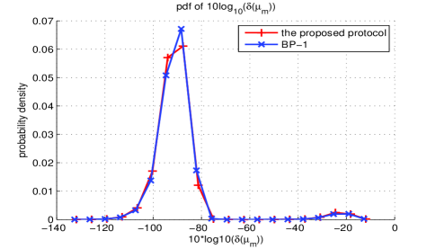
Figure 6: The PDF of $10*log10(\delta({\mu_{\rm u}})$ simulated over $10^{4}$ random system realizations.

To show the impact of relay position on the protocols’ performance, we choose $P_{\rm t}/\sigma^{2}=20$ dB and $K=32$, then evaluated the average optimum WSRs and $\frac{N_{\rm sp}}{K}$ for every protocol over $1000$ random channel realizations when $d$ increases from $0.1$ to $0.9$ km. Here, $N_{\rm sp}$ denotes the average number of the subcarrier pairs that should be used in the relay-aided mode to maximize the WSR. It can readily be computed that at most $20$ iterations is executed for Algorithm 1 for every channel realization generated. The results are shown in Figure 7.

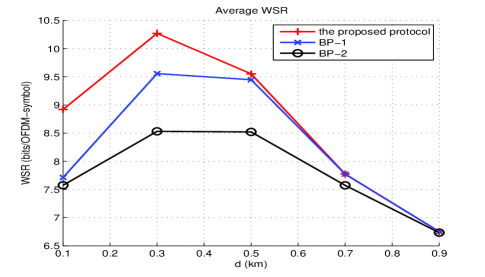
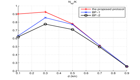
Figure 7: The average optimum WSRs and $\frac{N_{\rm sp}}{K}$ as the relay position changes when $P_{\rm t}/\sigma^{2}=20$ dB and $K=32$.

When $d$ is fixed, the proposed protocol leads to a greater average optimum WSR than BP-1, which illustrates the theoretical analysis in Section III-B. Moreover, the proposed protocol and BP-1 both have greater average optimum WSRs than BP-2. This is because they can better exploit the degrees of freedom for subcarrier pairing and assignment to users than BP-2 to improve the spectrum efficiency.

It is interesting to observe that for every protocol, the optimum WSR is higher and it is more likely to pair subcarriers for the relay-aided transmission to maximize the WSR when the relay moves toward the middle between the source and the user-region center. This behavior is interpreted for the proposed protocol as follows (those for BP-1 and BP-2 can be interpreted in a similar way and thus omitted due to space limitation). It is important to note that the optimum WSR for the proposed protocol, as the optimum objective value of (P1), depends on $\{G_{\mathrm{s}u,k},G^{\rm n}_{klu}|\forall\;k,l,u\}$. If $\forall\;k,l,u$, $G^{\rm n}_{klu}$ is more likely to take a high value, the subcarriers are more likely to be paired for the relay-aided transmission to maximize the WSR, and the average optimum WSR for the proposed protocol increases. As can be seen from Fig. 3, $G^{\rm n}_{klu}$ is high if both $G_{\mathrm{sr},k}$ and $G_{u,l}$ are much greater than $G_{\mathrm{s}u,k}$. When the relay lies in the middle between the source and the user-region center, both $G_{\mathrm{sr},k}$ and $G_{u,l}$ are likely to be much greater than $G_{\mathrm{s}u,k}$, meaning that $G^{\rm n}_{klu}$ is likely to be high. Therefore, the optimum WSR is higher and it is more likely to pair subcarriers for the relay-aided transmission when the relay lies in the middle between the source and the user-region center.

When $d$ is small, the optimum WSR for the proposed protocol is much greater than that for BP-1, and it is more likely to pair subcarriers for the relay-aided transmission to maximize the WSR for the proposed protocol than for BP-1. This can be explained as follows. Note that if $G^{\rm n}_{klu}-G^{\rm b}_{klu}$ is very likely to be high $\forall\;k,l,u$, the proposed protocol is more likely to pair the subcarriers for the relay-aided transmission than BP-1. According to the analysis in Section III-B, $G^{\rm n}_{klu}-G^{\rm b}_{klu}$ increases when $G_{\mathrm{sr},k}$ increases or $G_{\mathrm{r}u,l}$ reduces. When $d$ is small, $G_{\mathrm{sr},k}$ and $G_{\mathrm{r}u,l}$ are very likely to be high and small, respectively, meaning that $G^{\rm n}_{klu}-G^{\rm b}_{klu}$ is very likely to take a high value. This explains the observation.

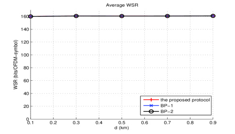
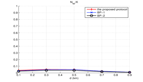
Figure 8: The average optimum WSRs and $\frac{N_{\rm sp}}{K}$ as the relay position changes when $P_{\rm t}/\sigma^{2}=45$ dB and $K=32$.

We also evaluated the average optimum WSRs and $\frac{N_{\rm sp}}{K}$ for every protocol over $1000$ random channel realizations when $P_{\rm t}/\sigma^{2}=45$ dB and $K=32$. It can readily be computed that at most $12$ iterations is executed for Algorithm 1 for every channel realization generated. The results are shown in Figure 8. It can be seen that regardless of the relay position, almost all subcarriers are used for the direct transmission to maximize the WSR for every protocol, therefore all protocols have similar average optimum WSRs. This can be interpreted as follows. Note that when the subcarrier pairing and assignment to users are fixed for every protocol, the optimum sum power for the subcarrier pairs and the optimum power for unpaired subcarriers can be found by the water-filling method. Since $P_{\rm t}/\sigma^{2}$ is very high, the optimum sum power allocated to subcarriers $k$ and $l$ is very likely to be high if they are paired for the relay-aided transmission to a user. In such a case, it can readily be shown that splitting this high sum power to the two subcarriers for separate direct transmission to the same user can result in a higher WSR. This explains why almost all subcarriers are used for the direct transmission to maximize the WSR when $P_{\rm t}/\sigma^{2}$ is very high. It also indicates that the proposed protocol leads to a better optimum WSR performance than the benchmark ones especially for the low-power regime.

VI Conclusion

In this paper, we have addressed the WSR maximization problem for the DF relay-aided downlink OFDMA transmission under a total power constraint. A novel subcarrier-pair based opportunistic DF relaying protocol has been proposed. A benchmark protocol has also be considered. An algorithm has been designed to find at least an approximately optimum RA with a WSR very close to the maximum WSR. Numerical experiments have illustrated the effectiveness of the RA algorithm and the impact of relay position and total power on the protocols’ performance. Theoretical analysis have been presented to interpret what were observed in numerical experiments.

Tao Wang received respectively Bachelor (summa cum laude) and Doctor of Engineering degrees from Zhejiang University, China, in 2001 and 2006, respectively, as well as Electrical Engineering degree (summa cum laude) and Ph.D from Université Catholique de Louvain (UCL), Belgium, in 2008 and 2012, respectively. He has been with School of Communication & Information Engineering, Shanghai University, China as a full professor since Feb. 2013, after winning Professor of Special Appointment (Eastern Scholar) Award from Shanghai Municipal Education Commission. Before that, he had multiple research appointments in UCL, Delft University of Technology and Holst Center in the Netherlands, Institute for Infocomm Research (I2R) in Singapore, and Motorola Electronics Ltd. Suzhou Branch in China. He is an associate editor for EURASIP Journal on Wireless Communications and Networking and Signal Processing: An International Journal (SPIJ), as well as an editorial board member of Recent Patents on Telecommunications. He served as a session chair in 2012 IEEE International Conference on Communications, and as a TPC member of International Congress on Image and Signal Processing in 2012 and 2010. He is an IEEE Senior Member.

François Glineur received engineering degrees from Faculté Polytechnique de Mons (Belgium) and École supérieure d’électricité (France) in 1997, and a Ph.D. in applied sciences from Faculté Polytechnique de Mons in 2001. He is currently professor of applied mathematics at the Engineering School of Université catholique de Louvain, member of the Center for Operations Research and Econometrics and the Institute of Information and Communication Technologies, Electronics and Applied Mathematics. His main research interests lie in convex optimization, including models, algorithms and applications, as well as in nonnegative matrix factorization.

Jérôme Louveaux received the electrical engineering degree and the Ph. D. degree from the Universit catholique de Louvain (UCL), Louvain-la-Neuve, Belgium in 1996 and 2000 respectively. From 2000 to 2001, he was a visiting scholar in the Electrical Engineering department at Stanford University, CA. From 2004 to 2005, he was a postdoctoral researcher at the Delft University of technology, Netherlands. Since 2006, he has been an Associate Professor in the ICTEAM institute at UCL. His research interests are in signal processing for digital communications, and in particular: xDSL systems, resource allocation, synchronization/estimation, and multicarrier modulations. Prof. Louveaux was a co-recipient of the ”Prix biennal Siemens 2000” for a contribution on filter-bank based multi-carrier transmission and co-recipient of the the ”Prix Scientifique Alcatel 2005” for a contribution in the field of powerline communications.

Luc Vandendorpe was born in Mouscron, Belgium in 1962. He received the Electrical Engineering degree (summa cum laude) and the Ph. D. degree from the Universit?Catholique de Louvain (UCL) Louvain-la-Neuve, Belgium in 1985 and 1991 respectively. Since 1985, he is with the Communications and Remote Sensing Laboratory of UCL where he first worked in the field of bit rate reduction techniques for video coding. In 1992, he was a Visiting Scientist and Research Fellow at the Telecommunications and Traffic Control Systems Group of the Delft Technical University, The Netherlands, where he worked on Spread Spectrum Techniques for Personal Communications Systems. From October 1992 to August 1997, L. Vandendorpe was Senior Research Associate of the Belgian NSF at UCL, and invited assistant professor. Presently he is Professor and head of the Institute for Information and Communication Technologies, Electronics and Applied Mathematics. His current interest is in digital communication systems and more precisely resource allocation for OFDM(A) based multicell systems, MIMO and distributed MIMO, sensor networks, turbo-based communications systems, physical layer security and UWB based positioning. In 1990, he was co-recipient of the Biennal Alcatel-Bell Award from the Belgian NSF for a contribution in the field of image coding. In 2000 he was co-recipient (with J. Louveaux and F. Deryck) of the Biennal Siemens Award from the Belgian NSF for a contribution about filter bank based multicarrier transmission. In 2004 he was co-winner (with J. Czyz) of the Face Authentication Competition, FAC 2004. L. Vandendorpe is or has been TPC member for numerous IEEE conferences (VTC Fall, Globecom Communications Theory Symposium, SPAWC, ICC) and for the Turbo Symposium. He was co-technical chair (with P. Duhamel) for IEEE ICASSP 2006. He was an editor of the IEEE Trans. on Communications for Synchronisation and Equalization between 2000 and 2002, associate editor of the IEEE Trans. on Wireless Communications between 2003 and 2005, and associate editor of the IEEE Trans. on Signal Processing between 2004 and 2006. He was chair of the IEEE Benelux joint chapter on Communications and Vehicular Technology between 1999 and 2003. He was an elected member of the Signal Processing for Communications committee between 2000 and 2005, and an elected member of the Sensor Array and Multichannel Signal Processing committee of the Signal Processing Society between 2006 and 2008. He was an elected member of the Signal Processing for Communications committee between 2000 and 2005, and between 2009 and 2011, and an elected member of the Sensor Array and Multichannel Signal Processing committee of the Signal Processing Society between 2006 and 2008. He is the Editor in Chief for the EURASIP Journal on Wireless Communications and Networking and a Fellow of the IEEE.

References

- [1] T. Wang and L. Vandendorpe, “On the SCALE algorithm for multiuser multicarrier power spectrum management,” IEEE Trans. Signal Process., vol. 60, no. 9, pp. 4992–4998, Aug. 2012.
- [2] ——, “Successive convex approximation based methods for dynamic spectrum management,” in 2012 IEEE Int. Conf. on Commun., Jun. 2012, pp. 4061–4065.
- [3] ——, “Iterative resource allocation for maximizing weighted sum min-rate in downlink cellular OFDMA systems,” IEEE Trans. Signal Process., vol. 59, no. 1, pp. 223–234, Jan. 2011.
- [4] Y. Liu, M. Tao, B. Li, and H. Shen, “Optimization framework and graph-based approach for relay-assisted bidirectional ofdma cellular networks,” IEEE Trans. Wireless Commun., vol. 9, no. 11, pp. 3490–3500, Nov. 2010.
- [5] A. Hottinen and T. Heikkinen, “Subchannel assignment in ofdm relay nodes,” in Proc. Information Sciences and Systems, Mar. 2006, pp. 1314–1317.
- [6] M. Herdin, “A chunk based ofdm amplify-and-forward relaying scheme for 4g mobile radio systems,” in IEEE Int. Conf. Commun., Jun. 2006, pp. 4507–4512.
- [7] I. Hammerstrom and A. Wittneben, “Power allocation schemes for amplify-and-forward mimo-ofdm relay links,” IEEE Trans. Wirel. Commun., vol. 6, no. 8, pp. 2798 –2802, Aug. 2007.
- [8] W. Dang, M. Tao, H. Mu, and J. Huang, “Subcarrier-pair based resource allocation for cooperative multi-relay ofdm systems,” IEEE Trans. Wirel. Commun., vol. 9, no. 5, pp. 1640 –1649, May 2010.
- [9] W. Wang, S. Yan, and S. Yang, “Optimally joint subcarrier matching and power allocation in ofdm multihop system,” EURASIP J. on Adv.in Sign. Proc., vol. 2008, pp. 1–8, 2008.
- [10] W. Wang and R. Wu, “Capacity maximization for ofdm two-hop relay system with separate power constraints,” IEEE Trans. Veh. Tech., vol. 58, no. 9, pp. 4943–4954, Nov. 2009.
- [11] Y. Li, W. Wang, J. Kong, and M. Peng, “Subcarrier pairing for amplify-and-forward and decode-and-forward ofdm relay links,” IEEE Commun. Lett., vol. 13, no. 4, pp. 209 –211, Apr. 2009.
- [12] T. Wang, “Weighted sum power minimization for multichannel decode-and-forward relaying,” IET Electronics Letters, vol. 48, no. 7, pp. 410–411, Apr. 2012.
- [13] L. Vandendorpe, R. Duran, J. Louveaux et al., “Power allocation for OFDM transmission with DF relaying,” in IEEE Int. Conf. Commun., May 2008, pp. 3795–3800.
- [14] J. Louveaux, R. Duran, and L. Vandendorpe, “Efficient algorithm for optimal power allocation in ofdm transmission with relaying,” in ICASSP, Mar. 2008, pp. 3257–3260.
- [15] T. C.-Y. Ng and W. Yu, “Joint optimization of relay strategies and resource allocations in cooperative cellular networks,” IEEE J. Sel. Areas on Commun., vol. 25, no. 2, pp. 328 –339, Feb. 2007.
- [16] Y. Wang, X. Qu, T. Wu, and B. Liu, “Power allocation and subcarrier pairing algorithm for regenerative ofdm relay system,” in IEEE Veh. Techn. Conf., Apr. 2007, pp. 2727–2731.
- [17] Y. Li, W. Wang, J. Kong et al., “Power allocation and subcarrier pairing in OFDM-based relaying networks,” in IEEE Int. Conf. Commun., May 2008, pp. 2602–2606.
- [18] M. Hajiaghayi, M. Dong, and B. Liang, “Optimal channel assignment and power allocation for dual-hop multi-channel multi-user relaying,” in Proc. IEEE INFOCOM, Apr. 2011, pp. 76 –80.
- [19] Z. Jin, T. Wang, J. Wei, and L. Vandendorpe, “Resource allocation for maximizing weighted sum of per cell min-rate in multi-cell DF relay aided downlink ofdma systems,” in 2012 IEEE-PIMRC, Sept. 2012, pp. 1845–1850.
- [20] ——, “A low-complexity resource allocation algorithm in multi-cell DF relay aided OFDMA systems,” in 2013 IEEE-WCNC, Apr. 2013.
- [21] L. Vandendorpe, J. Louveaux, O. Oguz et al., “Improved OFDM transmission with DF relaying and power allocation for a sum power constraint,” in ISWPC, 2008, pp. 665–669.
- [22] ——, “Power allocation for improved DF relayed OFDM transmission: the individual power constraint case,” in IEEE Int. Conf. Commun., 2009, pp. 1–6.
- [23] ——, “Rate-optimized power allocation for DF-relayed OFDM transmission under sum and individual power constraints,” Eurasip J. on Wirel. Commun. and Networking, vol. 2009.
- [24] C.-N. Hsu, H.-J. Su, and P.-H. Lin, “Joint subcarrier pairing and power allocation for OFDM transmission with decode-and-forward relaying,” IEEE Trans. Sig. Proc., vol. 59, no. 1, pp. 399–414, Jan. 2011.
- [25] T. Wang and L. Vandendorpe, “WSR maximized resource allocation in multiple DF relays aided OFDMA downlink transmission,” IEEE Trans. Sig. Proc., vol. 59, no. 8, pp. 3964 –3976, Aug. 2011.
- [26] ——, “Sum rate maximized resource allocation in multiple DF relays aided OFDM transmission,” IEEE J. Sel. Areas on Commun., vol. 29, no. 8, pp. 1559 –1571, Sep. 2011.
- [27] H. Boostanimehr and V. Bhargava, “Selective subcarrier pairing and power allocation for DF OFDM relay systems with perfect and partial CSI,” IEEE Trans. Wirel. Commun., vol. 10, no. 12, pp. 4057 –4067, Dec. 2011.
- [28] Y. Liu and M. Tao, “An optimal graph approach for optimizing ofdma relay networks,” in 2012 IEEE-ICC, Jun 2012.
- [29] T. Wang, Y. Fang, and L. Vandendorpe, “Power minimization for OFDM transmission with subcarrier-pair based opportunistic DF relaying,” IEEE Communications Letters, vol. 17, no. 2, 2013.
- [30] D. Tse and P. Viswanath, Fundamentals of Wireless Communication. Cambridge University Press, 2005.
- [31] W. Yu and R. Lui, “Dual methods for nonconvex spectrum optimization of multicarrier systems,” IEEE Trans. Commun., vol. 54, no. 7, pp. 1310–1322, July 2006.
- [32] K. Seong, M. Mohseni, and J. Cioffi, “Optimal resource allocation for OFDMA downlink systems,” in Proc. IEEE Int. Symp. Inf. Theory, july 2006, pp. 1394–1398.
- [33] W. Yu and J. Cioffi, “FDMA capacity of gaussian multiple-access channels with ISI,” IEEE Trans. Commun., vol. 50, no. 1, pp. 102–111, Jan. 2002.
- [34] L. Hoo, B. Halder, J. Tellado, and J. Cioffi, “Multiuser transmit optimization for multicarrier broadcast channels: asymptotic FDMA capacity region and algorithms,” IEEE Trans. Commun., vol. 52, no. 6, pp. 922–930, June 2004.
- [35] S. Boyd and L. Vandenberghe, Convex optimization. Cambridge University Press, 2004.
- [36] D. P. Bertsekas, Nonlinear programming, nd edition. Athena Scientific, 2003.
- [37] H. Khun, “The hungarian method for the assignment problems,” Naval Research Logistics Quarterly 2, pp. 83–97, 1955.