Clustering Via Nonparametric Density Estimation: the R Package pdfCluster

Adelchi Azzalini, Giovanna Menardi Clustering Via Nonparametric Density Estimation: the R Package pdfCluster Clustering Via Nonparametric Density Estimation The R package pdfCluster performs cluster analysis based on a nonparametric estimate of the density of the observed variables. After summarizing the main aspects of the methodology, we describe the features and the usage of the package, and finally illustrate its working with the aid of two datasets. cluster analysis, nonparametric density estimation, kernel methods, R, unsupervised classification, Delaunay triangulation cluster analysis, nonparametric density estimation, kernel methods, R, unsupervised classification, Delaunay triangulation Adelchi Azzalini
Dipartimento di Scienze Statistiche
Università di Padova, Italia
E-mail:
URL: http://azzalini.stat.unipd.it Giovanna Menardi
Dipartimento di Scienze Statistiche
Università di Padova, Italia
E-mail:

1 Clustering and density estimation

The traditional approach to the clustering problem, also called ‘unsupervised classification’ in the machine learning literature, hinges on some notion of distance or dissimilarity between objects. Once one such notion has been adopted among the many existing alternatives, the clustering process aims at grouping together objects having small dissimilarity, placing instead those with large dissimilarity in different groups. The classical reference for this approach is Hartigan (1975); the current standard account is Kaufman and Rousseeuw (1990).

In more recent years, substantial work has been directed to the idea that the objects to be clustered represent a sample from some $d$-dimensional random variable $X$ and the clustering process can consequently be carried out on the basis of the distribution of $X$, to be estimated from the data themselves. It is usually assumed that $X$ is of continuous type; denote its density function by $f(x)$, for $x\in\mathbb{R}^{d}$. We shall discuss later how the assumption that $X$ is continuous can be circumvented.

The above broad scheme can be developed in at least two distinct directions. The first one regards $X$ as a mixture of, say, $J$ subpopulations, so that its density function takes the form

$$f(x)=\sum_{j=1}^{J}\pi_{j}\,f_{j}(x)$$ (1)

where $f_{j}$ denotes the density function of the $j$-th subpopulation and $\pi_{j}$ represents its relative weight; here $\pi_{j}>0$ and $\sum_{j}\pi_{j}=1$. In this logic, a cluster is associated to each component $f_{j}$ and any given observation $x^{\prime}$ is allocated to the cluster with maximal density $f_{j}(x^{\prime})$ among the $J$ components.

To render the estimation problem identifiable, some restriction must be placed on the $f_{j}$’s. This is tipically achieved by assuming some parametric form for the component densities, whence the term ‘model-based clustering’ for this formulation, which largely overlaps with the notion of finite mixture modelling of a distribution. Quite naturally, the most common assumption for the $f_{j}$’s is of Gaussian type, but other families have also been considered. The estimation problem now involves estimation of the $\pi_{j}$’s and the set of parameters which identify each of $f_{1},\dots,f_{J}$ within the adopted parametric class. An extended treatment of finite mixture models is given by McLachlan and Peel (2000).

There exist some variants of the above mixture approach, but we do not dwell on them, since our main focus of interest is in the alternative direction which places the notion of density function in a nonparametric context. The chief motivation for this choice is to free the individual clusters from a given density shape, that is the parametric class adopted for the components $f_{j}$ in Equation 1. If the cluster shapes do not match the ones of the $f_{j}$’s, the mixture approach may face difficulties. This problem can be alleviated by adopting a parametric family of distributions more flexible than the Gaussian one. For instance, Lin et al. (2007) adopt the skew-$t$ distribution for the $f_{j}$ components; this family provides better adaptability to the data behaviour, and correspondingly can lead to a reduced number $J$ of components, compared to the Gaussian assumption. Although variants of this type certainly increase the flexibility of the approach, there is still motivation for considering a nonparametric formulation, completely free from assumptions on the cluster shapes.

The alternative approach to the use of density function in clustering places then $f(x)$ in a nonparametric context. Since this direction has been examined relatively more recently than the parametric one, it is undoubtedly less developed, but growing. It is not our purpose here to provide a systematic review of this literature, especially in the present setting, considering that very few of the methodologies proposed so far have lead to the construction of a broadly-usable software. We restrict ourselves to mention the works of Stuetzle (2003) and Stuetzle and Nugent (2010). In the supplementary material provided by this latter reference, the R package gslclust is also available. Among the few ready-to-use techniques, a quite popular one is ‘dbscan’ by Ester et al. (1996), originated in the machine learning literature and available through the R package fpc (Hennig, 2010); the notion of data density which they adopt is somewhat different from the one of probability theory considered here. For more information on the existing contributions in this stream of literature, we refer the reader to the discussion included in the papers to be summarized in the following section.

It is appropriate to clarify that the above two approaches involve somewhat different notions of cluster. In the nonparametric context, clusters are associated to regions with high density, while in the parametric setting (1) they are associated to the components $f_{j}$. The two concepts are different, even if they often lead effectively to the same outcome. A typical case where they diverge is provided by the mixture of two bivariate normal populations, both with markedly non-spherical distribution, such that where their tails overlap an additional mode, besides the centres of two normal components, is generated by the superposition of the densities; see for instance Figure 1 of Ray and Lindsay (2005) for a graphical illustration of this situation. In this case, the mixture model (1) declares that two clusters exist, while from the nonparametric viewpoint, where subpopulations do not feature, the three modes translates into three clusters.

The present paper focuses on the clustering methodology constructed via nonparametric density estimation developed by Azzalini and Torelli (2007) and by Menardi and Azzalini (2012). Of this formulation, we first recall the main components of the methodology and then describe its R implementation (R Development Core Team, 2012) in the package pdfCluster (Azzalini et al., 2012), illustrated with some numerical examples.

2 Clustering via nonparametric density estimation

2.1 Basic notions

The idea of associating clusters to modes or to regions of high density goes back a long time. Wishart (1969) stated that clustering methods should be able to identify “distinct data modes, independently of their shapes and variance”. Hartigan (1975, p. 205) stated that “clusters may be thought of as regions of high density separated from other such regions by regions of low density”, and the subsequent passage expanded somewhat this point by considering ‘density-contour’ clusters formed by regions with density above a given threshold $c$, and showing that these regions form a tree as $c$ varies. However, this direction was left unexplored and the rest of Hartigan’s book, as well as the subsequent mainstream literature, developed cluster analysis methodology in another direction, that is building on the notion of dissimilarity.

Among the few subsequent efforts to build clustering methods based on the idea of density function in a nonparametric context, we concentrate on the construction of Azzalini and Torelli (2007) and its development of Menardi and Azzalini (2012), which we summarize up to some minor differences.

For a $d$-dimensional density function $f(\cdot)$, which we assume to satisfy adequate regularity conditions, define

$$R(c) = \{x:x\in\mathbb{R}^{d},f(x)\geq c\},\qquad(0\leq c\leq\max f),$$ (2)

$$p_{c} = \int_{R(c)}f(x)\,\mathrm{d}x$$

which represent the region with density values above a level $c$ and its probability, respectively. For any given $c$, $R(c)$ may be a connected set or not; in the latter case, we have detected the presence of two or more high-density regions.

These notions are illustrated for the case $d=1$ by the left panel of Figure 1, where the two intervals at the basis of the shaded area jointly represent $R(c)$ and the area itself represents $p_{c}$, for a specific choice of $c$. As $c$ varies, the number of connected regions varies. Since $c$ and $p_{c}$ are monotonically related, we can regard the number of connected regions as a step function $m(p)$ of $p$, for $0<p<1$; for convenience, we set $m(0)=m(1)=0$. The right panel of Figure 1 displays the function $m(p)$ corresponding to the density of the left panel.

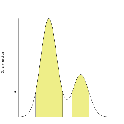
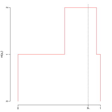
Figure 1: Density function and set $R(c)$ for a given $c$ (left panel) and corresponding mode function (right panel).

We shall refer to $m(p)$ as the ‘mode function’ because it enjoyes some useful properties related to the modes of $f(x)$. The most relevant facts are: (a) the total number of increments of $m(p)$, counted with their multiplicity, is equal to the number of modes, $M$; (b) a similar statement holds for the number of decrements; (c) the increment of $m(p)$ at a given point $p$ equals the number of modes whose ordinate is $c_{p}$. Inspection of the mode function allows to see, moving along the $p$ axis, when a new mode is given ‘birth’, or when two or more disconnected high-density sets merge into one.

Moreover, as established by Hartigan (1975, Section 11.13), the set of regions $R(c)$ exhibits a hierarchical structure. This tree structure will be illustrated later in the examples to follow.

When a set of observations $S=\{x_{1},\dots,x_{n}\}$ randomly sampled from $X$ is available, we can compute a nonparametric estimate $\hat{f}(x)$ of the density. The specific choice of the type of estimate is not crucial at this point, provided it satisfies commonly required properties of nonparametric estimates. The sample version $\hat{R}(c)$ of $R(c)$ is then obtained replacing $f(x)$ by $\hat{f}(x)$ in Equation 2, and a corresponding sample version of the mode function is introduced. Under mild regularity conditions, one can prove ‘strong set consistency’ of $\hat{R}(c)$ to $R(c)$, as $n\to\infty$.

Since we are primarity interested in allocating observations to clusters, far more often than allocating all points of $\mathbb{R}^{d}$, this can be achieved considering

$$S(c) = \{x_{i}:x_{i}\in S,\hat{f}(x_{i})\geq c\},\qquad(0\leq c\leq\max\hat{f}),$$ (3)

$$\hat{p}_{c} = |S(c)|/n$$

where $|\cdot|$ denotes cardinality of a set. Again, under mild conditions, one can show that $\hat{p}_{c}\to p_{c}$ as $n\to\infty$.

The above construction is conceptually simple and clear, but its actual implementation is problematic. While for $d=1$ identification of $R(c)$ and of $S(c)$ is elementary, as perceivable from Figure 1, the problem complicates substantially for $d>1$, which of course is the really interesting case. More specifically, it is immediate to state whether any given point $x$ belongs to any given set $R(c)$, but it is harder to say how many connected sets comprise $R(c)$, and which one they are; a similar problem exists for $S(c)$. The next two sections describe two routes to tackle this question.

2.2 Spatial tessellation

To establish whether a set $S(c)$ is formed by points belonging to one or more connected regions which comprise $\hat{R}(c)$, Azzalini and Torelli (2007) make use of some concepts from computational geometry. The first of these is the Voronoi tessellation which partitions the Euclidean space into $n$ polyhedra, possibly unbounded, each formed by those points of $\mathbb{R}^{d}$ which are closer to one given point in $S$ than to the others. Conceptually, from here one derives the Delaunay triangulation which is formed by joining points of $S$ which share a facet in the Voronoi tessellation. From a computational viewpoint, the Delaunay triangulation can be obtained directly, without forming the Voronoi tessellation first, and it is the only one required for the subsequent steps. The elements of the Delaunay triangulation are simplices in $\mathbb{R}^{d}$; since for $d=2$ they reduce to triangles, this explain the term.

These notions are illustrated in left panel of Figure 2 which shows the Voronoi tessellation and the Delaunay triangulation, for a set of points in $\mathbb{R}^{2}$.

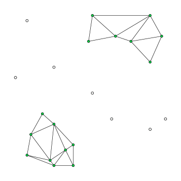
Figure 2: The left plot displays an example of Voronoi tessellation (dashed lines) for a set of points when $d=2$, and superimposed Delaunay triangulation (continuous lines). The right plot removes edges of some points from the original Delaunay triangulation, keeping points with $\hat{f}>c$ for some threshold $c$.

The procedure of Azzalini and Torelli (2007) consists of two main stages. The first one comprises itself a few steps, as follows. First, we construct the Delaunay triangulation of the sample $S$, and compute the nonparametric estimate $\hat{f}(x_{i})$ for each $x_{i}\in S$. Then, for any given value $p_{c}\in(0,1)$, we eliminate all points $x_{i}$ such that $\hat{f}(x_{i})<c$ and determine the connected sets of the remaining points. This step is illustrated graphically in the right panel of Figure 2, where two connected sets are visible after removing the points of low density and the associated arcs from the triangulation on the left panel. In principle, this operation is repeated for all possible values $p_{c}\in(0,1)$, in practice for a grid of such points. At the end of this process, we can construct a tree of these connected sets, provided we have kept track of the group membership of the sample components as $p_{c}$ ranges from $0$ to $1$. In the same process, we have also singled out $M$, say, groups of points which form the connected sets so identified; we call them ‘cluster cores’. It is a quite distinctive feature of this method to pinpoint a number $M$ of groups, while most methods require that $M$ is specified on input or it is left undetermined, like in hierarchical distance-based methods.

The outcome of the first stage is illustrated in Figure 3 for a set of simulated data with $d=2$. The left panel displays the observations points, marked with different symbols for the four cluster cores; the unlabelled points are denoted by a simple dot. The right panel shows the cluster tree of the four groups. Notice that the tree is upside-down with respect to the density: the root of the tree corresponds to zero density and the top mode, marked by 1, is near the bottom. This confirms that it would make more sense if mathematical trees had they roots at the bottom, like real trees.

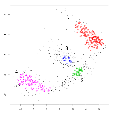
Figure 3: Cluster cores and cluster tree for a set of simulated data with $d=2$. In the left panel the points belonging to the custer chores are marked as follows: $1=\mathrm{o}$, $2=\triangle$, $3=+$, $4=\times$; the unlabelled points are marked by dots. The right panel shows the corresponding cluster tree.

In the second stage of the procedure, the points still unlabelled must be allocated among the $M$ cluster cores. This operation is a sort of classification problem, although of a peculiar type, since the unlabelled points are not randomly sampled from $X$, but inevitably in the outskirts of the cluster cores. Among the many alternative options, the proposed criterion is based on density estimation and density ratios. For an unlabelled point $x_{0}$, compute an estimate $\hat{f}_{m}(x_{0})$ of its density with respect to each of the cluster cores, that is for $m=1,\dots,M$, and assign $x_{0}$ to the group with highest log-ratio

$$r_{m}(x_{0})=\log\frac{\hat{f}_{m}(x_{0})}{\max_{k\not=m}\hat{f}_{k}(x_{0})}\,.$$ (4)

It is also proposed not to compute the estimates of the cluster cores densities $\hat{f}_{m}(\cdot)$ once for all, but to update them in a block-sequential matter, after a certain fraction of points has been allocated, and so on repeatedly for a given number of such blocks.

A variant of this allocation rule, not examined by Azzalini and Torelli (2007), but which we have found preferable on the whole, weights the the log-ratios in Equation 4 inversely with their variability while defining the order of allocation of the low density data. In practice, computation of the standard error of (4) is quite complicated, even employing asymptotic expressions of variances. We take a rough approximation of those quantities, instead, by first identifying the index $m^{\prime}$ such that $\hat{f}_{m^{\prime}}(x_{0})=\max_{k\not=m}\hat{f}_{k}(x_{0})$ and then considering the $m^{\prime}$ index as given. Next, we apply standard approximations for transformation of variables; see Bowman and Azzalini (1997, page 29), for the specific case of transforming $\hat{f}(\cdot)$.

As a diagnostic device to evaluate the quality of the clusters so obtained, the density-based silhouette (dbs) proposed by Menardi (2011) fits naturally in this framework. This tool is the analogue of the classical silhouette information (Rousseeuw, 1987), when the distances among points are replaced by probability log-ratios. Specifically, on defining for observation $x_{i}$,

$$\hat{\tau}_{m}(x_{i})=\frac{\pi_{m}\hat{f}_{m}(x_{i})}{\sum_{k=1}^{M}\pi_{k}\hat{f}_{k}(x_{i})},\qquad m=1,\ldots,M,$$

where $\pi_{m}$ is a prior probability for the $m$-th group, the dbs for $x_{i}$ is

$$\mbox{\emph{dbs}}_{i}=\frac{\log\left(\frac{\hat{\tau}_{m_{0}}(x_{i})}{\hat{\tau}_{m_{1}}(x_{i})}\right)}{{\max}_{x_{i}}\left|\log\left(\frac{\hat{\tau}_{m_{0}}(x_{i})}{\hat{\tau}_{m_{1}}(x_{i})}\right)\right|},$$

where $m_{0}$ is the group to which $x_{i}$ has been allocated and $m_{1}$ is the alternative group for which $\tau_{m}(x_{i})$ is maximal. The interpretation of the dbs diagnostics is the same as for the classical ‘silhouette’.

We close this section with some remarks on computational aspects. From the point of view of memory usage, the requirement of this procedure grows linearly with $n$, while for methods based on dissimilarities it grows quadratically. The more critical aspect here is construction of the Delaunay triangulation. This can be produced by the Quickhull algorithm by Barber et al. (1996), whose implementation is publicly available at http://www.qhull.org. This algorithm works efficiently for increasing $n$ when $d$ is small to moderate, but computing time grows exponentially when $d$ increases.

2.3 Pairwise connections

The final remarks of the previous section motivate the development of a variant procedure to build a connection network of the elements of $S$ by using a different criterion instead of the Delaunay triangulation, leaving unchanged the rest of the above-described process.

The proposal of Menardi and Azzalini (2012) starts by reconsidering the notion of connected sets for $d=1$ and then extending this view to the case $d>1$. The basic idea is to examine the behaviour of $\hat{f}(x)$ when we move along a segment $[x_{1},x_{2}]$, since it depends on whether the sample values $x_{1}$ and $x_{2}$ belong to the same connected set of $\hat{R}(c)$ or not. To visualize the process, it is convenient to refer to the left panel of Figure 1, regarding the density there as the estimate $\hat{f}$, and consider the set $\hat{R}(c)$ formed by the union of the two intervals of the shaded area. If $x_{1}$ and $x_{2}$ belong to the same interval, then the corresponding portion of density along the segment $(x_{1},x_{2})$ has no local minimum. On the contrary, if $x_{1}$ and $x_{2}$ belong to different subsets of $\hat{R}(c)$, then at some point along $[x_{1},x_{2}]$ the density exhibits a local minimum, which we shall refer to as ‘presence of a valley’.

When $d>1$, the same idea can be carried over by examining the behaviour of the section of $\hat{f}(x)$ along the segment joining $x_{1}$ and $x_{2}$ where $x_{1},x_{2}\in\mathbb{R}^{d}$ and applying the same principle as above. A graph is then created whose vertices are the sample points and an arc is set between any pair of points such that there is no valley in the section of $\hat{f}(x)$ between them.

In practical terms, the claim of presence of a valley must allow some tolerance for the inevitable variability of $\hat{f}$. Given the above premises, we must take into account the amplitude of the valley detected along the stated section of $\hat{f}$, and declare that $x_{1}$ and $x_{2}$ are connected points if this amplitude is below a certain threshold. Clearly, if no valley exists, the connection of $x_{1}$ and $x_{2}$ is unquestioned.

This broad idea of tolerance must be given a specific form to be operational. Menardi and Azzalini (2012) adopt a criterion which for simplicity we only describe informally, and refer the reader to their paper for full specification. When a valley is detected, we introduce an auxiliary function derived from the original one by increasing it by the minimum amount required to fill the valley; one can think that water is poured into the valley until it starts to overflow. To visualize this process, consider Figure 4 where, in the first panel, a sample of points in $\mathbb{R}^{2}$ is depicted and the segments joining two pairs of them, $(x_{1},x_{2})$ and $(x_{3},x_{4})$, are highlighted. The second panel displays the section of $\hat{f}(x)$ along the segment joining $x_{1}$ and $x_{2}$, represented by the smooth curve, and the auxiliary function which fills the valley. The amplitute of the valley in this case is quantified by

$$R=\frac{\mbox{integral of the dark-shaded area}}{\mbox{integral of the dark-shaded area $+$ integral of the light-shaded area}}\in[0,1).$$

If $R<\lambda$, for a given tolerance parameter $\lambda\in(0,1)$, $x_{1}$ and $x_{2}$ are considered connected points, and an edge is set in the connection graph. For the pair $(x_{3},x_{4})$ in Figure 4, the section of $\hat{f}(x)$ along the segment joining them is concave (plot not shown); hence in this case $R=0$ and the points are declared to be connected.

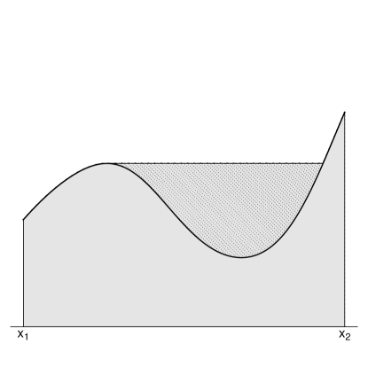
Figure 4: The left panel displays a set of points in $\mathbb{R}^{2}$, of which two pairs, $(x_{1},x_{2})$ and $(x_{3},x_{4})$, are highlighted by drawing the segment joining them. The right plot displays the section of $\hat{f}(x)$ along the segment which joins $x_{1}$ and $x_{2}$ (smooth curve delimiting the light-shaded area) and the associated auxiliary non-decreasing function (with filled area highlighted).

Once the connection of all pairs of sample values has been examined, the rest of the process is carried out exactly as in the previous section. Since now we are always working in a one-dimensional world, higher values of $d$ can be tackled. However, for large $d$ we are facing another problem: the degrade of performance of nonparametric density estimates, known as ‘course of dimensionality’. On the other hand, it can be argued that for the clustering problem we need to identify only the main features of a distribution, especially its modes, not the fine details. This consideration indicates than the method can be considered also for a broader set of cases than those where the density is the focus of interest. See Menardi and Azzalini (2012) for a more extended discussion of this issue.

3 The R package pdfCluster

3.1 Package overview

The R package pdfCluster performs, as its main task, cluster analysis by implementing the methodology described in the previous sections. Furthermore, two other tasks are accomplished: density estimation and clustering diagnostics.

Each of these tasks is associated with a set of functions and methods, and results in an object of a specific class, as summarized in Table 1. The package is built by making use of classes and methods of the S4 system.

	clustering	density estimation	diagnostics
S4 class	pdfCluster-class	kepdf-class	dbs-class
functions to produce the class	pdfCluster pdfClassification	kepdf	dbs
related methods	pdfCluster plot show summary	plot show summary	dbs plot show summary
others		h.norm hprop2f	adj.rand.index

Table 1: Summary of the pdfCluster package. Each of the three main tasks of the package is associated with a set of functions and methods, and results in an object of a specific S4 class.

To ease presentation, an overview of the package is first provided, aiming at an introductory usage of its features. The next section is devoted to a more in-depth examination of computational and technical details.

Clustering via nonparametric density estimation

The package is built around the main routine pdfCluster, which actually performs the clustering process. pdfCluster is defined as a generic function and dispatches different methods depending on the class of its first argument. For a simple use of this function, the user is only required to provide the data x to be clustered, in the form of a vector, matrix, or data.frame of numeric elements. A further method dispatched by the pdfCluster generic function applies to objects of pdfCluster-class itself. This last option will be discussed later.

Further arguments include graphtype, which defines the procedure to identify the connected components of the density level sets. The elementary case $d=1$ is handled by the "unidimensional" option. When data are multidimensional, instead, this argument may be set to "delaunay" or "pairs", to run the procedures, as described in Section 2.2 and 2.3, respectively. If not specified, the latter option is selected when the data dimension is greater than $6$. When "pairs" is selected, explicitly or implicitly, the user may wish to specify the parameter lambda, which defines the tolerance threshold to claim the presence of valleys in the section of $\hat{f}(x)$ between pairs of points. Default value is lambda=0.10.

After that the connected components associated with the density level sets are identified, pdfCluster builds the cluster tree and detects the cluster cores. An internal call to function pdfClassification follows by default, to carry on the second phase of the clustering procedure, that is allocation of the lower density data points not belonging to the cluster cores. The user can regulate the process of classification by setting some optional parameters to be passed to pdfClassification. Details are discussed below.

Further optional arguments may given to pdfCluster in order to regulate density estimation. These arguments are passed internally to function kepdf, which is described below.

The results of the clustering process are encapsulated in an object of pdfCluster-class, whose slots include, among others, a list nc providing details about the connected components identified for each considered section of the density estimate, a vector cluster.cores defining the cluster cores membership, and an object of class dendrogram, providing information about the cluster tree, the number noc of detected groups. Furthermore, when the classification procedure is carried on, the slot stages is a list with elements corresponding to the data allocation to groups at the different stages of the classification procedure and clusters reports the final group labels.

Methods to show, to provide a summary and to plot objects of pdfCluster-class are available. Four types of plot are selectable, by setting the argument which. Argument which=1 plots the mode function; which=2 plots the cluster tree; a scatterplot of the data or of pairs of selected coordinates reporting the label group is provided when which=3 and which=4 plots the density-based silhouette information as will be described below. Multiple choices are possible.

Density estimation

Density estimation is performed by the kernel method througout the kepdf function. Estimates are computed by a product estimator of the form:

$$\hat{f}(y)=\sum_{i=1}^{n}\frac{1}{nh_{i,j}\cdots h_{i,d}}\prod_{j=1}^{d}K\left(\frac{y_{j}-x_{i,j}}{h_{i,j}}\right).$$

The kernel function $K$ is an argument of function kepdf and can either be a Gaussian density (if kernel = "gaussian") or a $t_{\nu}$ density, with $\nu=7$ degrees of freedom (when kernel = "t7"). The uncommon option of selecting a $t$ distribution is motivated by computational reasons, as will be clarified in Section 3.2.

The user may choose to estimate density with a fixed or an adaptive bandwidth $h_{i}=(h_{i,1}\cdots h_{i,d})^{\prime}$, by setting the argument bwtype accordingly. Leaving the argument unspecified entails the use of a fixed bandwidth estimator. When bwtype="fixed", that is $h_{i}=h$, a constant smoothing vector is used for all the observations $x_{i}$. Default values are set as asymptotically optimal for a multivariate Normal distribution Bowman and Azzalini (see, e.g., 1997, page 32). Alternatively, bwtype="adaptive", which corresponds to specify a vector of bandwidths $h_{i}$ for each observation $x_{i}$. Default values are selected according to the approach described by Silverman (1986, Section 5.3.1), implemented in the package through the function hprop2f.

Results of the application of the kepdf function are encapsulated in objects of kepdf-class, whose slots include the estimate at the evaluation points and the parameters used to obtain that estimate.

Methods which show, provide a summary, and plot objects of kepdf-class are also available. When the density estimate is based on two or higher dimensional data, these functions make use of functions contour, image and persp, depending on how the argument method is set. When $d>2$, the pairwise marginal estimated densities are plotted for all pairs of coordinates, or for a subset of coordinates specified by the user via the argument indcol.

Diagnostics of clustering

As a third feature, the package provides diagnostics of the clustering outcome. Density-based silhouette is computed by the generic function dbs, which dispatches two methods. One method applies to objects of pdfCluster-class directly; a second method is thought to compute the density-based silhouette information on partitions produced by a possibly different density-based clustering technique. The latter method applies applies to two arguments: the matrix of clustered data and a numeric vector of cluster labels.

Computation of the density-based silhouette requires the density function to be estimated, conditional to the group membership. Hence, further arguments of function kepdf can be given to dbs to set parameters of density estimation. Moreover, some prior probability may be specified for each cluster.

Results of the application of function dbs are provided in objects of dbs-class. An S4 method for plotting objects of dbs-class is available: data are partitioned into the clusters, sorted in a decreasing order with respect to their dbs value and displayed on a bar graph.

As a further diagnostic tool, the package provides the function adj.rand.index which evaluates the agreement between two partitions, through the adjusted Rand criterion (Hubert and Arabie, 1985).

3.2 Further details

• As already mentioned, pdfCluster automatically selects the procedure to be used for detecting connected components of the density level sets, depending on the data dimensionality. While the user is allowed to change this choice by setting argument graphtype, we warn against setting the argument graphtype="delaunay" for large dimensions. The number of operations required to compute the Delaunay triangulation grows with $n^{\lfloor d/2\rfloor}$ while the computational complexity due to run the pairwise connection criterion grows quadratically with the sample size. Hence, at the present state of computing resourses, running the Delaunay triangulation when $d>6$ appears hardly feasible for values of $n$ greater than about $200$. Instead, data with any dimensionality may be handled by the pairwise connection criterion, although the computational speed slows down for very large $n$.

• The higher computational efficiency of the pairwise connection criterion is paid for by the need of setting the tolerance threshold $\lambda$. According to our experience, the default value of lambda=0.10 is usually a sensible choice for moderate to high dimension while a lower lambda is sufficient in low dimensions, when the density estimate is more accurate. A larger value can be useful when the procedure detects a number of small spurious groups, because this choice results in aggregating clusters.

• As running the procedure several times with different choices of lambda may be time consuming, the package allows for a more efficient route, implemented by an additional method dispatched by function pdfCluster. Once that an object of pdfCluster-class is created by function pdfCluster with argument graphtype= "pairs", pdfCluster can be called again by setting the same pdfCluster-class object as a first argument x and a different value of lambda: slot graph of the pdfCluster-class object contains the amplitude of the valleys detected by the evaluation of the density along the segments connecting observations. Then, the pairwise evaluation does not need to be run again to check results for different values of lambda and the procedure speeds up considerably. An example will be illustrated in the next section.

• Both the Delaunay and the pairwise connection criterion to build a graph on the observed data are implemented by some specifically designed foreign functions. In the former case, the delaunayn function in package geometry (Barber et al., 2012) is the R interface to the Quickhull algorithm. Pairwise connection is, instead, implemented in the C language.

• After building the selected connection network among the observations, pdfCluster determines the level set $S(c)$ for a grid of values of $p_{c}$; the length of such grid may be set through the n.grid argument. For each value of $p_{c}$ the identification of connected components of $S(c)$ is carried out by means of a C function borrowed by the R package spdep (Bivand et al., 2012), which implements a depth first search algorithm.

• The procedure to allocate the low density data to the cluster cores is block-sequential and the user is allowed to select the number n.stage of such blocks as an optional parameter of pdfCluster, to be passed internally to pdfClassification (default value is n.stage = 5). When this argument is set to $0$, the clustering process stops when the cluster cores are identified. Otherwise, further arguments can be passed from pdfCluster to pdfClassification. Among them, se takes "logical" values, and is set to TRUE to account for the standard error of the log-likelihood ratios in Equation 4. Argument hcores declares if the densities in (4) have to be estimated by selecting the same bandwidths as the ones used to form the cluster cores. Default value is set to FALSE, in which case a vector of bandwidth specific for the clusters is used.

• pdfCluster makes an internal call to function kepdf both to estimate the density underlying data and to build the connection network when the pairwise connection criterion is selected. By default, a kernel density estimation with fixed kernel is built, with vector of smoothing parameters set to the one asymptotically optimal under the assumption of multivariate normality. Although arguably sub-optimal, this choice produces sensible results in most applications. When dimensionality of data is low-to-moderate, it is often advantageous to shrink the smoothing parameter slightly towards zero; we adopt a shrinkage factor hmult=3/4 when $d\leq 6$, as recommended by Azzalini and Torelli (2007), but the default value may be optionally modified by the user. For higher-dimensional data, instead, we suggest the use of a kernel estimator with adaptive bandwidth, which can be obtained by setting argument bwtype to "adaptive".

• Function kepdf represents the R interface of two C routines which allow to speed computations. Each of these routines is designed to perform kernel density estimation with a specific kernel function. It is worth to remind that, when connected sets are identified by the pairwise connection criterion, computation of the $R$ measure in Equation 2.3 requires the density function to be evaluated along the segments joining each pair of observations. In practice, a grid of grid.pairs points is considered for each segment, so that the number of operation required grows with $n^{2}$grid.pairs .
  When sample size is very large, any saving in the arithmetic computations of the kernel can make a noticeable difference. In particular, the use of a Gaussian kernel requires a call to the exponential function at each evaluation, which is computationally much more expensive than sum, multiplication and power function. This explains the non-standard option to select a $t_{\nu}$ kernel, with $\nu=7$ degrees of freedom. The relatively more critical computation involves an $8$th degree power, which can be coded efficiently and still the kernel has unbounded support, which is more appropriate for the classification stage than alternatives like bisquare or similar kernels. The use of this option is then suggested when the sample size is huge.

• To compute dbs, it is possible to specify some prior probability of each cluster. To this end, recall that clusters are labelled according to the maximal value of the density, so that label $1$ refers to the cluster with overall maximal density. The choice depends on the prior knowledge about the composition of the clusters and a lack of information would imply the choice of a uniform distribution over the groups. However, information derived from the detected partition can also be used. When diagnostics are computed on an object of pdfCluster-class, prior probabilities can be chosen as proportional to the cardinalities of the cluster cores. This is also the default choice. In a model-based clustering, instead, the mixing proportions could be a natural choice.

4 Some illustrative examples

4.1 Quantitative variables

The wine data set was introduced by Forina et al. (1986). It originally included the results of 27 chemical measurements on 178 wines grown in the same region in Italy but derived from three different cultivars: Barolo, Grignolino and Barbera. The pdfCluster package provides a selection of 13 variables. The data set is here used to illustrate the main features of the package.

As a first simple example, let us suppose to have some knowledge about which variables are relevant to the aim of reconstructing the cultivar of origin of each wine. We then perform cluster analysis on a small subset of variables. R> library("pdfCluster") R> data("wine") R> winesub <- wine[, c(2,5,8)] As the number of considered variables is very small, visual exploration of the density estimate of the data may already give us some indication about the clustering structure. R> pdf <- kepdf(winesub) R> plot(pdf, text.diag.panel= names(winesub)) The resulting plot is displayed in Figure 5. A three-cluster structure is clearly evident from the marginal density estimate of the variables "Alcohol" and "Flavanoids". The main content of the kepdf-class object pdf may be printed by the associated show method. R> pdf An S4 object of class "kepdf"

Call: kepdf(x = winesub)

Kernel: [1] "gaussian"

Estimator type: fixed bandwidth

Diagonal elements of the smothing matrix: 0.3750856 1.542968 0.4614995

Density estimate at evaluation points: [1] 0.015211471 0.001994922 0.009822658 0.010526400 0.009014892 0.013104296 [7] 0.005910667 0.013900582 …

Figure 5: Plot of the pairwise marginal density estimates of three variables of wine data, as given by function kepdf.

Clustering is performed by a call to pdfCluster. Note that its usage does not require a preliminary call to kepdf. A summary of the resulting object provides the cardinalities of both the cluster cores and the clusters, along with the main structure of the cluster tree. R> cl.winesub <- pdfCluster(winesub) R> summary(cl.winesub) An S4 object of class "pdfCluster"

Initial groupings: label: 1 2 3 NA count: 29 13 17 119

Final groupings: label: 1 2 3 count: 62 63 53

Groups tree: –[dendrogram w/ 1 branches and 3 members at h = 1] ‘–[dendrogram w/ 2 branches and 3 members at h = 0.36] |–leaf "1 " ‘–[dendrogram w/ 2 branches and 2 members at h = 0.32] |–leaf "2 " (h= 0.04 ) ‘–leaf "3 " (h= 0.06 )

The object may be further inspected by accessing its slots. Slot graph, for instance, discloses the procedure used to find the connected components associated to the level set: R> cl.winesub@graph

$type
[1] "delaunay"

The user may be also interested about details regarding the estimated density, available through the slot pdf. R> cl.winesub@pdf

$kernel
[1] "gaussian"

$bwtype
[1] "fixed"

$par
$par$h
   Alcohol Alcalinity Flavanoids
 0.2813142  1.1572259  0.3461246

$par$hx
NULL

$estimate
  [1] 0.021153490 0.003723019 0.009561598 0.013346244 0.011821547 0.017818041
  [7] 0.006527976 0.017082718 ...

Note that the vector of smoothing parameters used to estimate density, during the process of clustering, differs from the one produced by the previous call to function kepdf, whose default value is asymptotically optimal for Normal data, as given by function h.norm(). As already mentioned, when low-dimensional data are clustered (in this example $d=3$), this vector is multiplied by a shrinkage factor of $3/4$ by default.

Additional information about the detected partition may be further visualized through a call to the associated plot methods. If argument which is not selected, the four available types of plot are displayed one at a time.

R> plot(cl.winesub) The resulting plots are reported in Figure 6. In particular, the diagnostic plot presents values of the dbs appreciably larger than zero for almost all the observations throughout the three clusters, suggesting the soundness of the detected partition. This is confirmed by the cross-classification frequencies of the the obtained clusters and the actual cultivar of origin of the wines (indicated in the first column of the wine data). R> table(wine[,1], cl.winesub@clusters) 1 2 3 Barolo 58 1 0 Grignolino 4 62 5 Barbera 0 0 48

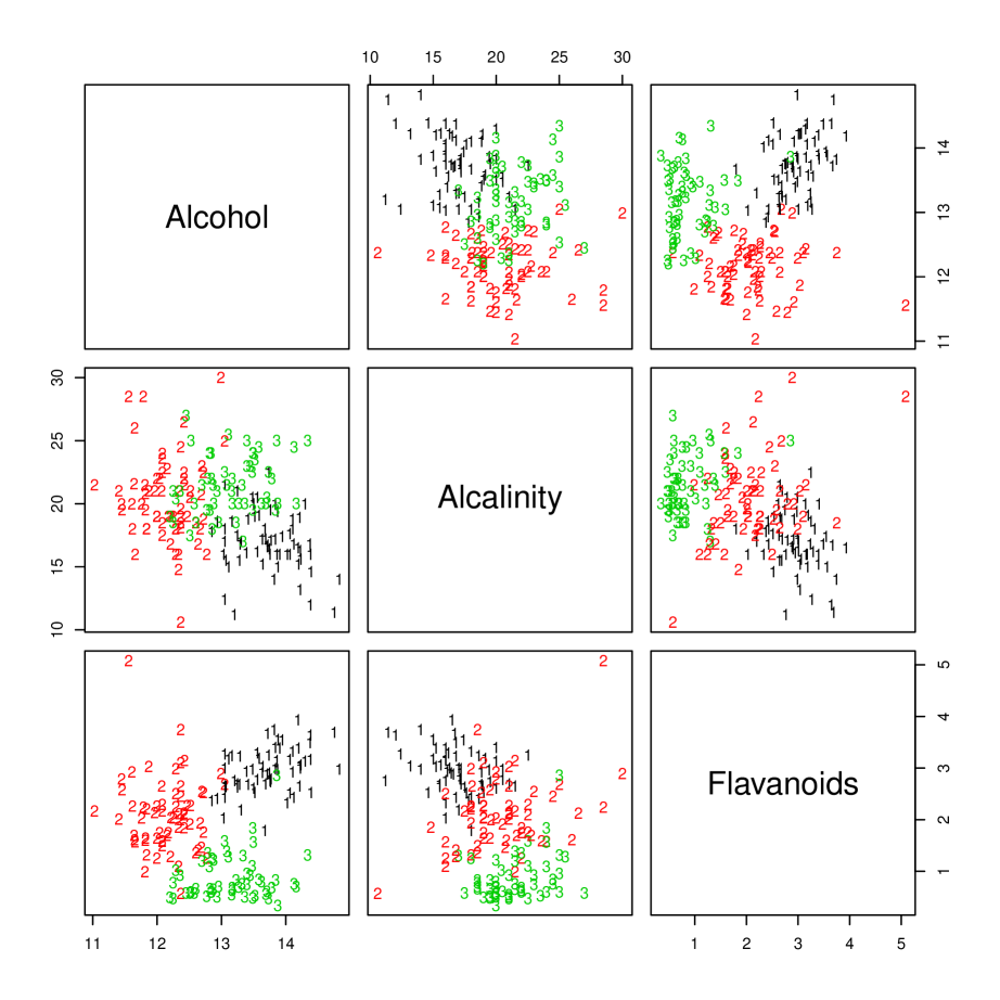
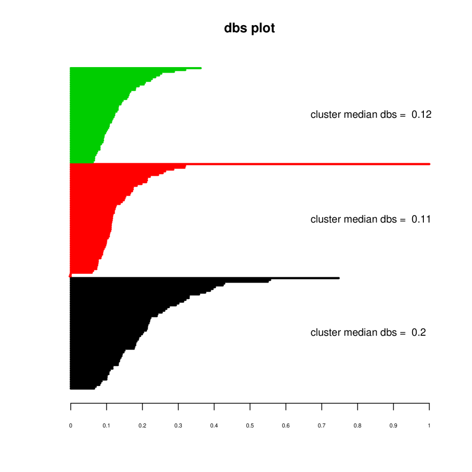
Figure 6: Result of the application of plot methods on objects of pdfCluster-class. From the left: the mode function, the cluster tree, the pairwise scatterplot and the dbs plot.

Consider now the entire data set wine (we only remove the true label class of wines). R> wineall <- wine [, -1] When high-dimensional data are clustered, some caution should be used to deal with the curse of dimensionality and the increased variability of the density estimate. Menardi and Azzalini (2012) suggest either to allow for different amount of smoothing by using an adaptive bandwidth, or to oversmooth the density: R> cl.wineall <-pdfCluster(wineall, bwtype="adaptive") R> summary(cl.wineall) An S4 object of class "pdfCluster"

Initial groupings: label: 1 2 3 4 5 6 NA count: 5 2 10 4 5 3 149

Final groupings: label: 1 2 3 4 5 6 count: 35 32 36 40 20 15

Groups tree: –[dendrogram w/ 1 branches and 6 members at h = 1] ‘–[dendrogram w/ 2 branches and 6 members at h = 0.62] |–[dendrogram w/ 1 branches and 4 members at h = 0.32] | ‘–[dendrogram w/ 3 branches and 4 members at h = 0.28] | |–[dendrogram w/ 2 branches and 2 members at h = 0.04] | | |–leaf "2 " (h= 0.02 ) | | ‘–leaf "1 " | |–leaf "3 " (h= 0.12 ) | ‘–leaf "4 " (h= 0.12 ) ‘–[dendrogram w/ 2 branches and 2 members at h = 0.32] |–leaf "5 " (h= 0.14 ) ‘–leaf "6 " (h= 0.18 )

Note that six groups have now been produced. The identification of more than three clusters, when all the thirteen variables of the wine data are used, is consistent with results of the application of other clustering methods (see, e.g., McNicholas and Murphy, 2008). However, their pairwise aggregation as $\{1,2\},\{3,6\},\{4,5\}$ essentially leads to the three actual cultivars, with a few misclassified points left: R> table(wine[,1], cl.wineall@clusters) 1 2 3 4 5 6 Barolo 32 27 0 0 0 0 Grignolino 3 5 0 40 19 4 Barbera 0 0 36 0 1 11 A more accurate classification may be obtained by additionally employing oversmoothing the density: R> cl.wineall.os <-pdfCluster(wineall, bwtype="adaptive", hmult=1.2) R> table(wine[,1], cl.wineall.os@clusters) 1 2 3 Barolo 59 0 0 Grignolino 6 4 61 Barbera 0 47 1

A similar effect may be caused by relaxing the condition to set connections among points, while building the pairwise connection graph among the observations. In the current example, data dimensionality equal to $13$ has entitled the use of the pairwise connection criterion, as may be seen from: R> cl.wineall@graph[1:2] $type[1]"pairs"\par$lambda [1] 0.1

In addition to the criterion adopted to build the network connection, the slot graph reports the tolerance threshold lambda. The third, not displayed, element of the slot contains the amplitude of the valleys detected by the evaluation of the density along the segments connecting all the pairs of observations. A larger value of $\lambda$ typically results in aggregation of clusters, and can be obtained either by re-running the whole procedure: R> cl.wineall.l0.2 <- pdfCluster(wineall, bwtype = "adaptive", lambda = 0.2) or by applying the method which the pdfCluster function dispatches to pdfCluster-class objects: R> cl.wineall.l0.2 <- pdfCluster(cl.wineall, lambda = 0.2) The latter choice does not re-run pairwise evaluation and it exploits, instead, computations saved in the slot graph of the pdfCluster-class object. This speeds up the clustering procedure considerably, especially when the sample size is large.

4.2 Mixed variables

As they stand, density-based clustering methods may be applied to continuous data only. However, we illustrate here how this assumption may be circumvented.

Consider the data set plantTraits from package cluster (Maechler et al., 2005). It describes 136 plant species according to 31 morphological and reproductive attributes. R> library("cluster") R> data("plantTraits") In order to use all available information to cluster the data, a reasonable procedure seems to us as follows: first, a dissimilarity matrix among the points is created, using criteria commonly employed in classical distance-based methods; next, from this matrix, a configuration of points in the $d^{\prime}$-dimensional Euclidean space is sought by means of multidimensional scaling, for some given $d^{\prime}$. In this way, $d^{\prime}$ numerical coordinates are obtained, to be passed to the clustering procedure.

It is inevitable that any recoding procedure of this sort involves some arbitrarieness and the one just described is no exception. However, of the two steps involved, the first one is exactly that considered by classical hierarchical clustering techniques. The second step requires a few additional choices, especially the number $d^{\prime}$ of principal coordinates. A detailed exploration of these aspects is definitely beyond the scope of this paper and will be pursued elsewhere.

For the present illustrative purposes, we refer to the example reported in the documentation of the cluster package, and we choose the Gower coefficient to measure the dissimilarity among the points, implemented in R by function daisy. The categorical variables are distinguished in ordered, binary asymmetric and symmetric, and handled accordingly Kaufman and Rousseeuw (see 1990, Chapter 1). R> example(plantTraits) … plntTr> dai.b <- daisy(plantTraits, plntTr+ type = list(ordratio=4:11, symm=12:13, asymm=14:31)) We then make use of classical multidimensional scaling (Gower, 1966), which is computed by function cmdscale, and we take the simple option of setting $d^{\prime}=6$ as in Maechler et al. (2005). plntTr> cmdsdai.b <-cmdscale(dai.b, k=6) With the new set of data, we may run the clustering procedure. R> cl.plntTr <-pdfCluster(cmdsdai.b) R> summary(cl.plntTr) An S4 object of class "pdfCluster"

Initial groupings: label: 1 2 NA count: 23 2 111

Final groupings: label: 1 2 count: 128 8

Groups tree: –[dendrogram w/ 1 branches and 2 members at h = 1] ‘–[dendrogram w/ 2 branches and 2 members at h = 0.18] |–leaf "1 " ‘–leaf "2 " (h= 0.16 ) The outcome indicates the presence of two clusters. However, the number of data points assigned to one of the two clusters is very small, and the associated cluster core is formed by two observations only. In these circumstances, selecting a global bandwidth to classify the lower density data seems to be more appropriate than using cluster specific bandwidths. This can be pursued with the following commands: R> cl.plntTr.hc <-pdfCluster(cmdsdai.b, cores=TRUE) While the plantTraits data set does not include information about a true label class of the cases, it is interesting to note that the two identified groups roughly correspond to the aggregation of the clusters $\{1,3,5,6\}$ and $\{2,4\}$ identified by running a distance-based method and then cutting the dendrogram at six clusters, as suggested by Maechler et al. (2005). plntTr> agn.trts <- agnes(dai.b, method="ward") … plntTr> cutree6 <- cutree(agn.trts, k=6) R> table(cutree6, cl.plntTr.hc@clusters) cutree6 1 2 1 10 0 2 11 20 3 21 0 4 4 15 5 18 1 6 35 1 Note that selecting six principal coordinates places us at the threshold we defined to choose both the type procedure to find the connected level sets and the way of smoothing the density function. Since the threshold $d=6$ is merely indicative, in these circumstances it makes sense to check results deriving from a different setting of the arguments as, for example R> cl.plntTr.hc.newset <-pdfCluster(cmdsdai.b, cores=TRUE, graphtype="pairs", bwtype="adaptive") A variant procedure to handle mixed data would recode the categorical variables only, and run pdfCluster on the set of data obtained by merging the principal coordinates so constructed and the original quantitative variables.

References

- Azzalini et al. (2012) Azzalini A, Menardi G, Rosolin T (2012). \proglangR Package \pkgpdfCluster: Cluster Analysis Via Nonparametric Density Estimation (Version 1.0-0). Università di Padova, Italia. URL http://cran.r-project.org/web/packages/pdfCluster/index.html.
- Azzalini and Torelli (2007) Azzalini A, Torelli N (2007). “Clustering Via Nonparametric Density Estimation.” Statistics and Computing, 17, 71–80.
- Barber et al. (2012) Barber C, Habel K, Grasman R, Gramacy RB, Stahel A, Sterratt DC (2012). \pkgGeometry: Mesh Generation and Surface Tesselation. \proglangR Package Version 0.3-1, URL http://cran.r-project.org/web/packages/geometry/index.html.
- Barber et al. (1996) Barber CB, Dobkin DP, Huhdanpaa H (1996). “The Quickhull Algorithm for Convex Hulls.” ACM Transactions On Mathematicals Software, 22, 469–483.
- Bivand et al. (2012) Bivand R, with contributions by Altman M, Anselin L, Assunção R, Berke O, Bernat A, Blanchet G, Blankmeyer E, Carvalho M, Christensen B, Y C, Dormann C, Dray S, Halbersma R, Krainski E, Legendre P, Lewin-Koh N, Li H, Ma J, Millo G, Mueller W, Ono H, Peres-Neto P, Piras G, Reder M, Tiefelsdorf M, Yu D (2012). \pkgSpdep: Spatial Dependence: Weighting Schemes, Statistics and Models. \proglangR Package Version 0.5-46, URL http://cran.r-project.org/web/packages/spdep/index.html.
- Bowman and Azzalini (1997) Bowman AW, Azzalini A (1997). Applied Smoothing Techniques for Data Analysis: the Kernel Approach with S-Plus Illustrations. Oxford University Press, Oxford.
- Ester et al. (1996) Ester M, Kriegel H, Sander J, Xu X (1996). “A Density Based Algorithm For Discovering Clusters in Large Spatial Databases Withe Noise.” In Proceedings of the 2Nd International Conference On Knowledge Discovery and Data Mining (KDD-96). Aaai Press, Portland.
- Forina et al. (1986) Forina M, Armanino C, Castino M, Ubigli M (1986). “Multivariate Data Analysis As a Discriminating Method of the Origin of Wines.” Vitis, 25, 189–201.
- Gower (1966) Gower JC (1966). “Some Distance Properties of Latent Root and Vector Methods Used in Multivariate Analysis.” Biometrika, 53, 325–328.
- Hartigan (1975) Hartigan JA (1975). Clustering Algorithms. John Wiley & Sons, New York.
- Hennig (2010) Hennig C (2010). \pkgFpc: Flexible Procedures for Clustering. \proglangR Package Version 2.0-3, URL http://cran.r-project.org/web/packages/fpc/index.html.
- Hubert and Arabie (1985) Hubert L, Arabie P (1985). “Comparing Partitions.” Journal of Classification, 2, 193–218.
- Kaufman and Rousseeuw (1990) Kaufman L, Rousseeuw PJ (1990). Finding Groups in Data: An Introduction to Cluster Analysis. John Wiley & Sons, New York.
- Lin et al. (2007) Lin TI, Lee JC, Hsieh WJ (2007). “Robust Mixture Modeling Using the Skew Distribution.” Statistics and Computing, 17, 81–92.
- Maechler et al. (2005) Maechler M, Rousseeuw P, Struyf A, Hubert M (2005). “\pkgCluster: Cluster Analysis Basics and Extensions.” \proglangR package version 1.14.2, URL http://cran.r-project.org/web/packages/cluster/citation.html.
- McLachlan and Peel (2000) McLachlan GJ, Peel D (2000). Finite Mixture Models. John Wiley & Sons, New York.
- McNicholas and Murphy (2008) McNicholas PD, Murphy TB (2008). “Parsimonious Gaussian Mixture Models.” Statistics and Computing, 18, 285–296.
- Menardi (2011) Menardi G (2011). “Density-Based Silhouette Diagnostics for Clustering Methods.” Statistics and Computing, 21, 295–308.
- Menardi and Azzalini (2012) Menardi G, Azzalini A (2012). “An Advancement in Clustering Via Nonparametric Density Estimation.” Submitted.
- R Development Core Team (2012) R Development Core Team (2012). \proglangR: A Language and Environment for Statistical Computing. R Foundation for Statistical Computing, Vienna, Austria. ISBN 3-900051-07-0, URL http://www.R-project.org/.
- Ray and Lindsay (2005) Ray S, Lindsay BG (2005). “The Topography of Multivariate Normal Mixtures.” The Annals of Statistics, 33, 2042–2065.
- Rousseeuw (1987) Rousseeuw P (1987). “Silhouettes: A Graphical Aid to the Interpretation and Validation of Cluster Analysis.” Journal of Computational Applied Mathematics, 20, 53–65.
- Silverman (1986) Silverman BW (1986). Density Estimation for Statistics and Data Analysis. Chapman and Hall, London.
- Stuetzle (2003) Stuetzle W (2003). “Estimating the Cluster Tree of a Density by Analyzing the Minimal Spanning Tree of a Sample.” Journal of Classification, 20, 25–47.
- Stuetzle and Nugent (2010) Stuetzle W, Nugent R (2010). “A Generalized Single Linkage Method for Estimating the Cluster Tree of a Density.” Journal of Computational and Graphical Statistics, 19, 397–418.
- Wishart (1969) Wishart D (1969). “Mode Analysis: A Generalization of Nearest Neighbor Which Reduces Chaining Effects.” Numerical Taxonomy, pp. 282–308.