Emitting electrons spectra and acceleration processes in the jet of Mrk 421: from low state to giant flare state

Abstract

We investigate the electron energy distributions (EEDs) and the acceleration processes in the jet of Mrk 421 through fitting the spectral energy distributions (SEDs) in different active states in the frame of a one-zone synchrotron self-Compton (SSC) model. After assuming two possible EEDs formed in different acceleration models: the shock accelerated power-law with exponential cut-off (PLC) EED and the stochastic turbulence accelerated log-parabolic (LP) EED, we fit the observed SEDs of Mrk 421 in both low and giant flare states by using the Markov Chain Monte Carlo (MCMC) method which constrains the model parameters in a more efficient way. Our calculating results indicate that (1) the PLC and LP models give comparably good fits for the SED in low state, but the variations of model parameters from low state to flaring can be reasonably explained only in the case of the PLC in low state; and (2) the LP model gives better fits compared to the PLC model for the SED in flare state, and the intra-day/night variability observed at GeV-TeV bands can be accommodated only in the LP model. The giant flare may be attributed to the stochastic turbulence re-acceleration of the shock accelerated electrons in low state. Therefore, we may conclude that shock acceleration is dominant in low state, while stochastic turbulence acceleration is dominant in flare state. Moreover, our result shows that the extrapolated TeV spectra from the best-fit SEDs from optical through GeV with the two EEDs are different. It should be considered in caution when such extrapolated TeV spectra are used to constrain extragalactic background light (EBL) models.

1 Introduction

Blazars are the most extreme class of active galactic nucleies (AGNs). Their spectral energy distributions (SEDs) are characterized by two distinct bumps. The first bump, which is located at the low energy band from radio through UV or X-rays, is generally explained by the synchrotron emission from relativistic electrons in a jet that is closely aligned to the line of sight. The second bump, which is located at the high-energy band, could be produced by inverse Compton (IC) scattering of the relativistic electrons (the so-called leptonic model; e.g., Böttcher, 2007). The seed photons for IC process can be synchrotron photons (synchrotron self-Compton, SSC; Rees, 1967; Maraschi et al., 1992) or external radiation fields (EC; Dermer & Schlickeiser, 1993; Sikora et al., 1994). The hadronic model is an alternative explanation for the high energy emissions from blazars (e.g., Mannheim, 1993; Mücke et al., 2003; Dimitrakoudis et al., 2012; Dermer et al., 2012).

In the leptonic model, a power-law EED with an exponential high-energy cutoff (PLC), or a broken power-law EED is commonly adopted (e.g., Tavecchio et al., 1998; Finke et al., 2008). The main justification for this EED approximation is that the non-thermal emissions from blazars can be described by a power-law spectrum, and the power-law EED can be naturally generated in the framework of the shock acceleration (the Fermi I process) (e.g., Baring, 1997). In recent observations, however, the X-ray spectra of several blazars (like Mrk 421, Mrk 501) show significant curvature, which are typically milder than an exponential cut-off (Massaro et al., 2004a, b, 2006). Very recently, it has been found that gamma-ray emissions of many blazars are successfully fitted with a log-parabolic (LP) spectrum (e.g., Aharonian et al., 2009; Abdo et al., 2010; Ackermann et al., 2011). The LP EED is then proposed to model the observed spectral curvature, and such LP EED can be generated in the stochastic turbulence acceleration scenario (the Fermi II process) (e.g., Tramacere et al., 2009, 2011). Numerical simulation indicates that stochastic acceleration process may play an important role in the formation of the particle spectrum in blazar jet (Virtanen & Vainio, 2005). When the emission mechanisms are determined, the emitting EED can be reconstructed from the observed emission spectra. We can then investigate the acceleration processes acting in blazar jet (e.g., Ushio et al., 2010; Garson et al., 2010).

Blazars are well known for their rapid and large-amplitude variability at all wavebands, most prominently at keV and TeV energies. The relations (including correlation and time lag) between variabilities at different wavelengths are crucial for constraining jet models (e.g., Sokolov et al., 2004; Fossati et al., 2008; Katarzyński & Walczewska, 2010; Böttcher & Dermer, 2010). For instance, if the hard lag is observed, a acceleration process could be considered in the model. Different flare patterns indicate different causes of the flare, such as change in the injection rate and change in the acceleration process, etc (e.g., Kirk et al., 1998; Kataoka et al., 2000; Graff et al., 2008; Moraitis & Mastichiadis, 2011; Chen et al., 2011).

Mrk 421 is the closest known (redshift $z=$0.031) and the first very high energy (VHE) blazar (Punch et al., 1992). It is classified as high-peaked BL Lac (HBL) according to its synchrotron peak location. Mrk 421 is the main target of multi-wavelength monitoring campaigns. There are a large number of publications on the multi-wavelength observations of this source. Its SED and relation of variabilities at different bands are intensively studied (e.g., Błażejowski et al., 2005; Albert et al., 2007; Acciari et al., 2009, 2011; Aleksić et al., 2010; Bartoli et al., 2011). From these studies, we learned that TeV flare is often correlated with keV flare, however, such relation is very complex. For example, the TeV flux increases more than quadratically with respect to the X-ray one, and there is time lag between TeV and keV flares. Although SED of Mrk 421 is commonly well fitted by a one-zone SSC model, the complex variability behaviors remind us that the realistic model seems more complicated. Lately, the multi-wavelength campaign showed evidence for Mrk 421 in low/quiescent state from 2009 January 19 to 2009 June 1 (Abdo et al., 2011). During this campaign, no significant flare activity was seen and the measured VHE flux is among the lowest fluxes recorded by MAGIC. Abdo et al. (2011) therefore claimed that the unprecedented complete, 4.5 months average SED observed during this campaign can be considered as an excellent proxy for the low/quiescent state SED of Mrk 421. Several months later, Mrk 421 was found to undergo its one of the brightest outburst at X-rays and gamma-rays bands on February 17, 2010 (Shukla et al., 2012). During this flaring, the flux correlation at X-ray and TeV band was observed (Shukla et al., 2012), and intra-night variability at GeV - TeV band was found (Galante et al., 2011; Shukla et al., 2012; Raue et al., 2012).

In this paper we investigate the EEDs and the acceleration processes in the jet of Mrk 421 in low state and giant flare state. To achieve our aim, we assume two electron distributions, both well motivated by the current particle acceleration models: the shock accelerated PLC EED and the stochastic turbulence accelerated LP EED, to model the SEDs in the frame of a one-zone SSC model. To more efficiently constrain the model parameters and better distinguish between the models, we employ the Markov Chain Monte Carlo (MCMC) method instead of a simple $\chi^{2}$-minimization procedure to investigate the high-dimensional model parameter space systematically. The emission models and MCMC method are briefly described in Section 2. In Section 3, we report our results. Finally in Section 4 we summarize our discussions and conclusions.

2 Emission model and MCMC method

2.1 Emission model

The one-zone SSC assumes that non-thermal radiation is produced by both the synchrotron radiation and SSC process in a spherical blob filled with uniform magnetic field ($B$), which is moving relativistically at a small angle to our line of sight, and the observed radiation is strongly boosted by a relativistic Doppler factor $\delta_{\rm D}$. The radius of emitting blob is $R^{\prime}=\frac{t_{\rm v,min}\delta_{D}c}{1+z}$, where $t_{\rm v,min}$ is the minimum variability timescale. Here, quantities in the observer’s frame are unprimed, and quantities in the comoving frame are primed. Note that the magnetic field $B$ is defined in the comoving frame, despite being unprimed. We use the methods given in Finke et al. (2008) to calculate synchrotron and SSC fluxes.

The PLC electron distribution formed in the Fermi I acceleration process is

$$N^{\prime}(\gamma^{\prime})=K^{\prime}_{\rm e}\gamma^{\prime-s}\exp(\frac{-\gamma^{\prime}}{\gamma^{\prime}_{c}})\ \ {\rm for}\ \ \gamma^{\prime}_{\rm min}\leq\gamma^{\prime}\leq\gamma^{\prime}_{\rm max},$$ (1)

where $K^{\prime}_{\rm e}$ is the normalization of the EED, $s$ is the electron energy index, and $\gamma^{\prime}_{c}$ is the electron cut-off energy. $\gamma^{\prime}_{\rm min}$ and $\gamma^{\prime}_{\rm max}$ is the electron minimum energy and electron maximum energy, respectively. In this model, there are eight free parameters, five of them specify the electron energy distribution ($K^{\prime}_{e}$, $\gamma^{\prime}_{\rm min}$, $\gamma^{\prime}_{c}$, $\gamma^{\prime}_{\rm max}$, $s$) and the other three ones describe the global properties of the emitting region ($B$, $R^{\prime}$, $\delta_{D}$).

The LP electron distribution generated in the Fermi II acceleration process is

$$N^{\prime}(\gamma^{\prime})=K^{\prime}_{e}~{}\left\{\begin{array}[]{ll}\left(\frac{\gamma^{\prime}}{\gamma^{\prime}_{c}}\right)^{-s}&\gamma^{\prime}_{\rm min}\leq\gamma^{\prime}\leq\gamma^{\prime}_{c}\\ \left(\frac{\gamma^{\prime}}{\gamma^{\prime}_{c}}\right)^{-[s+r\log(\frac{\gamma^{\prime}}{\gamma^{\prime}_{c}})]}&\gamma^{\prime}_{c}\leq\gamma^{\prime}\leq\gamma^{\prime}_{\rm max}\;,\end{array}\right.$$ (2)

where $r$ is the curvature term of EED (Massaro et al., 2006). In this model, $r$ is an additional one besides the eight parameters mentioned above.

2.2 MCMC method

The MCMC method, based on the Bayesian statistics, is well suitable for high dimensional parameter space investigation, which is superior to the grid approach with a more efficient sampling of the parameter space of interest. The Metropolis-Hastings sampling algorithm is adopted to determine the jump probability from one point to the next in the parameter space (Mackay, 2003). The algorithm ensures that the probability density functions (PDF) of model parameters can be asymptotically approached with the number density of samples. In the following fitting, we will run single chains using the Raftery & Lewis convergence diagnostics (Raftery & Lewis, 1992), and we assume flat priors in the model parameters spaces. A brief introduction to the basic procedure of the MCMC sampling can be found in Fan et al. (2010). For more details about the MCMC method, please refer to Neal (1993); Gamerman (1997); Mackay (2003). Since the code we used in this paper (Liu et al., 2012) is adapted from COSMOMC, we refer the reader to the website and to Lewis & Bridle (2002) and references therein for a detailed explanation of the code about the sampling options, convergence criteria and statistical quantities.

3 Modeling results

3.1 Modeling the SED in low state

In this case, we adopt the optical-UV to X-ray data observed by Swift/UVOT/RXT/BAT and the Fermi-LAT gamma-rays data reported in Abdo et al. (2011). For the Fermi-LAT data, the last two data points are not included in our modeling, due to their very large uncertainties. Instead, we use the first two data points measured by MAGIC since the extragalactic background light (EBL) absorption on the flux at such energy band is negligible. Because the EBL absorption has an effect on the other fluxes measured by MAGIC, we also do not take them into account in our modeling. The absorption effect of EBL will be discussed in §3.3. The SMA data at $2.3\times 10^{11}$ Hz are used to constrain $\gamma^{\prime}_{\rm min}$. We fix $\gamma^{\prime}_{\rm min}=700$ for PLC case and $\gamma^{\prime}_{\rm min}=1200$ for LP case and $\gamma^{\prime}_{\rm max}=10^{8}$ for both case.

For the PLC electron distribution, the one-dimensional (1D) probability distributions and two-dimensional (2D) confidence regions (at 1$\sigma$ and 2$\sigma$ confidence levels) of the model parameters, and the SED are shown in Fig. 1. The fitting parameters are summarized in Table 1 with the reduced $\chi^{2}_{\nu}=1.01$ for 27 d.o.f. (Note that a relative systematic uncertainty of 5% was added in quadrature to the statistical error of the optical-UV-X-rays data reported in Abdo et al. (2011)). It can be seen that a very good constraint is derived for the spectral energy index $s$. The parameters $\gamma^{\prime}_{c}$, $K^{\prime}_{e}$ and $\delta_{\rm D}$ are well constrained. The constraints on $B$ and $t_{\rm v,min}$ are not strong, but they are still restricted in relatively small ranges.

For the 2D confidence regions of the parameters, we only show some combinations with relatively large correlations. It can be seen that there are negative correlations between $\gamma^{\prime}_{c}$ and $B$, $B$ and $\delta_{\rm D}$, as well as $t_{\rm v,min}$ and $\delta_{\rm D}$, but there are positive correlations between $K^{\prime}_{e}$ and $t_{\rm v,min}$ and between $K^{\prime}_{e}$ and $\gamma^{\prime}_{c}$. In the following, we try to physically understand the correlations among some parameters. In the standard SSC model, the synchrotron SED peak flux in the $\delta$-approximation is $\nu F_{\nu}\propto N^{\prime}(\gamma^{\prime}_{\rm c})B^{2}\gamma^{\prime 3}_{\rm c}\delta^{4}_{\rm D}$ and the synchrotron peak energy is $E_{\rm s}\propto\gamma^{\prime 2}_{\rm c}B\delta_{\rm D}$ (e.g., Tramacere et al., 2011). The negative correlation between $\gamma^{\prime}_{\rm c}$ and $B$ is predicted for the constant $E_{\rm s}$ which can be estimated by the observed spectra. Because $B\delta_{\rm D}\propto\nu^{2}_{\rm s}/\nu_{\rm c}$ in the SSC model in the Thomson regime (e.g., Tavecchio et al., 1998), where $\nu_{\rm s}$ and $\nu_{\rm c}$ are the peak frequencies of the synchrotron and IC scattering respectively, the negative correlation between $B$ and $\delta_{\rm D}$ is expected for the observed $\nu_{\rm s}$ and $\nu_{\rm c}$, which implies that the IC scattering is in the Thomson regime. In the SSC model, the radius $R^{\prime}$ of the emitting blob relates to the gamma-ray flux ($\propto R^{\prime-2}$) and then can be estimated using the observed gamma-ray flux, meanwhile $R^{\prime}\sim c\delta_{\rm D}t_{\rm v,min}$, hence a negative correlation between $t_{\rm v,min}$ and $\delta_{\rm D}$ can be predicted. On the other hand, with $B\propto E_{\rm s}/(\gamma^{\prime 2}_{\rm c}\delta_{\rm D})$, the synchrotron peak flux can be rewritten as $(\nu F_{\nu})_{\rm s}\propto(K^{\prime}_{\rm e}/\gamma^{\prime}_{\rm c})\delta^{2}_{\rm D}E^{2}_{\rm s}$, therefore the positive correlation between $K^{\prime}_{\rm e}$ and $\gamma^{\prime}_{\rm c}$ is expected by the constraint of the observed synchrotron peak flux. As to the positive correlation between $K^{\prime}_{e}$ and $t_{\rm v,min}$, since IC peak flux $(\nu F_{\nu})_{\rm c}$ can be estimated by using the observed gamma-ray flux and $(\nu F_{\nu})_{\rm c}/(\nu F_{\nu})_{\rm s}\propto K^{\prime}_{e}/\delta^{2}_{\rm D}t^{2}_{\rm v,min}$, and then $K^{\prime}_{e}/t_{\rm v,min}\propto[(\nu F_{\nu})_{\rm c}/(\nu F_{\nu})_{\rm s}][\nu_{\rm c}/\nu^{2}_{\rm s}]$ where $t_{\rm v,min}B\delta^{3}_{\rm D}=\rm constant$ and $B\delta_{\rm D}\propto\nu^{2}_{\rm s}/\nu_{\rm c}$ (Tavecchio et al., 1998) are used. Therefore, the positive correlation between $K^{\prime}_{e}$ and $t_{\rm v,min}$ can be predicted according to the observations.

For the LP electron distribution, the parameters distributions and SED are shown in Fig. 2. The fitting parameters are listed in Table 1. In this case, we have $\chi^{2}_{\nu}=0.97$ (for 26 d.o.f.). The curvature term $r$ is well constrained. It seems that $B$ can be better constrained than that in PLC model. The constraints on the other parameters are similar to that derived in the PLC model. The explanations on the correlations in the case of PLC still hold in the case of LP except for the correlation between $B$ and $\gamma^{\prime}_{c}$. In LP case, the correlation between $B$ and $\gamma^{\prime}_{c}$ becomes weak, which is caused by the effect of $r$ . This correlation between $B$ and $r$ is caused by the well-observed spectrum around the synchrotron peak.

Comparing the results derived in the two EEDs, it can be found that the global properties of the emitting blob ($B$, $\delta_{\rm D}$, $R^{\prime}$) derived in the two cases are comparable. Obviously, we cannot distinguish between the PLC and LP electron distributions in the low state based on the above results (see Figs. 1 and 2 as well as Table 1).

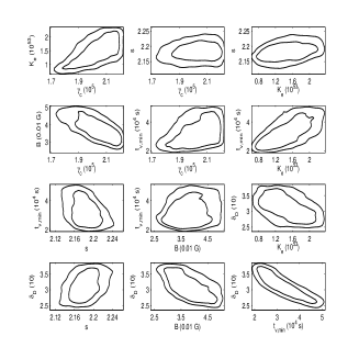
Figure 1: Modeling the SED in low state with the PLC electron distribution. Left: 1-D marginalized probability distribution of the parameters. The solid vertical line is the expected value, and the 68% limits are depicted by the dashed vertical lines; Middle: 2-D confidence contours of the parameters. The contours are for 1 and 2$\sigma$ levels; Right: the best fit to the SED from optical-UV-X-ray to GeV bands. For the low energy component, the symbols represent Swift/UVOT (squares), RXT (circles) and BAT (diamonds) data; For high energy component, the symbols represent Fermi-LAT (circles) and MAGIC (diamonds) data. For the detailed information of the observed data sets, please refer to Abdo et al. (2011).

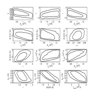
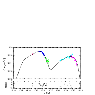
Figure 2: Same as in Fig. 1 but with the LP electron distribution.

Table 1: Fitting parameters for the SED in low state.

Model	$\gamma^{\prime}_{c}$	$K^{\prime}_{e}$	$s$	$r$	$B$	$t_{\rm v,min}$	$\delta_{\rm D}$	$U^{\prime}_{e}/U^{\prime}_{B}$
	($10^{5}$)	($10^{53}$/$10^{42}$)			(0.01 G)	($10^{4}$ s)	(10)
PLC model	2.02$\pm$0.11	1.48$\pm$0.39	2.19$\pm$0.02	–	3.81$\pm$0.56	3.30$\pm$0.75	3.12$\pm$0.32	34.61
68% limit	(1.90 - 2.20)	(1.04 - 1.91)	(2.16 - 2.21)	–	(3.22 - 4.45)	(2.50 - 4.18)	(2.77 - 3.49)
LP model	1.47$\pm$0.08	0.93$\pm$0.16	2.43$\pm$0.02	1.68$\pm$0.10	2.05$\pm$0.38	4.90$\pm$0.60	3.34$\pm$0.25	50.71
68% limit	(1.37 - 1.60)	(0.70 - 1.12)	(2.41 - 2.45)	(1.58 - 1.78)	(1.65 - 2.47)	(4.26 - 5.57)	(3.07 - 3.62)

3.2 Modeling the SED in flare state

For the SED in flaring state, the Swift/RXT, RXTE/PCA, Fermi-LAT and HAGAR data reported in Shukla et al. (2012) are adopted. We also fix $\gamma^{\prime}_{\rm min}$ and $\gamma^{\prime}_{\rm max}$ as we did in Section 3.1. The parameters distributions and SED fitting derived with PLC EED are shown in Fig. 3. The fitting parameters are listed in Table 2. The resulting $\chi^{2}_{\nu}=0.79$ for 318 d.o.f. is below unity after a relative systematic uncertainty of 8% was added. The fittings at optical and GeV bands are bad. $\gamma^{\prime}_{c}$ and $s$ are well constrained, and $t_{\rm v,min}$ can be constrained in relatively small range. However, the parameters $K^{\prime}_{e}$, $\delta_{\rm D}$ and $B$ are poorly constrained. We cannot obtain the meaningful distribution ranges of the three parameters, thus only the 68% upper limit are reported in Table 2. Unfortunately, the variability timescale ($\sim 1$ day) required in this PLC model contradicts the observed intra-day variability at GeV - TeV bands (Shukla et al., 2012; Raue et al., 2012).

Compared to the results in PLC case, it can be seen from Fig. 4 that the fittings with LP EED is significantly improved with $\chi^{2}_{\nu}=0.30$ (for 317 d.o.f.). Besides, relatively better constraints are obtained for all parameters, especially for $s$, $r$, $\gamma^{\prime}_{c}$ and $K^{\prime}_{e}$. Furthermore, the LP model with required $t_{\rm v,min}\sim 8$ hours can accommodate the intra-day/night variability observed at GeV - TeV bands. It should be noted that the interpretations of the correlations of parameters in Section 3.1 still hold here.

Table 2: Fitting parameters for the SED in giant flare state.

Model	$\gamma^{\prime}_{c}$	$K^{\prime}_{e}$	$s$	$r$	$B$	$t_{v,min}$	$\delta_{D}$	$U^{\prime}_{e}/U^{\prime}_{B}$
	($10^{5}$)	($10^{53}$/$10^{42}$)			(0.01 G)	($10^{4}$ s)	(10)
PLC model	5.82$\pm$0.14	0.04$\pm$0.01	1.65$\pm$0.01	–	1.07$\pm$0.06	7.98$\pm$0.55	2.99$\pm$0.08	110.08
68% limit	(5.66 - 5.97)	( $<$0.04)	(1.64 - 1.66)	–	( $<$1.14)	(7.36 - 8.57)	($<3.07$)
LP model	3.63$\pm$0.21	0.17$\pm$0.03	2.02$\pm$0.04	3.79$\pm$0.26	2.67$\pm$0.32	2.66$\pm$0.32	3.44$\pm$0.20	61.75
68% limit	(3.42 - 3.86)	(0.14 - 0.20)	(1.99 - 2.06)	(3.51 - 4.08)	(2.30 - 3.03)	(2.30 - 3.02)	(3.22 - 3.66)

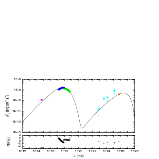
Figure 3: Modeling the SED in giant flare state with the PLC electron distribution. The curves are the same as that in Fig. 1. For low energy component of SED, the symbols denote the data from SPOL CCD Imaging/Spectropolarimeter at Steward Observatory (squares), the XRT data (circles) and the PCA data (triangles); At high energy component, the symbols denote LAT data (circles) and HAGAR data (triangle). Please see Shukla et al. (2012) for more details about the data sets.

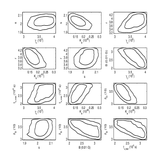
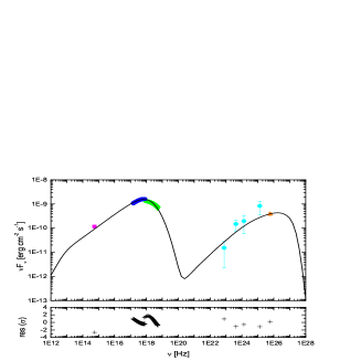
Figure 4: Modeling the SED in giant flare state with the LP electron distribution. The curves are the same as that in Fig. 1, and the symbols are the same as that in Fig. 3.

3.3 From low state to giant flare state

After determining the EED in flare state, we can discuss the EED in low state through investigating the variations of model parameters with activities. Tramacere et al. (2007, 2009) studied the spectral energy distributions (SEDs) of Mrk 421 in different states in the frame of the SSC model and found that there is a negative correlation between the curvature parameter of the radiation spectrum $b\approx r/5$ and $E_{\rm s}$, which is expected from the stochastic acceleration mechanism. Tramacere et al. (2011) pointed out that the observed negative correlation can be explained by the variation of the momentum diffusion coefficient $D_{p}(\gamma)=D_{p0}(\gamma/\gamma_{0})^{q}$, where $q$ is the turbulence spectrum index (note that a larger value of $D_{p}$ implies higher acceleration rate), or the fact that the corresponding EEDs are far from the equilibrium where the acceleration dominates over the radiative cooling. They also suggested that the curvature increases as the radiative cooling becomes important and EED is approaching to the equilibrium during the evolution of EED. From Tables 1 and 2, if we assume that EEDs in low and giant states both have the LP shapes, we find that $\gamma^{\prime}_{c}=1.47\times 10^{5}$, $B=2.05\times 10^{-2}$ G, $\delta_{\rm D}=34.4$, and $r=1.68$ in the low state, and $\gamma^{\prime}_{c}=3.63\times 10^{5}$, $B=2.67\times 10^{-2}$ G, $\delta_{\rm D}=33.4$, and $r=3.79$ in the giant state. Therefore, the ratios of synchrotron peak energies and the curvature parameters in two states are $[E_{\rm s}]_{\rm giant}/[E_{\rm s}]_{\rm low}=[\gamma^{\prime 2}_{\rm c}B\delta_{\rm D}]_{\rm giant}/[\gamma^{\prime 2}_{\rm c}B\delta_{\rm D}]_{\rm low}\approx 7.7$ and $[r]_{\rm giant}/[r]_{\rm low}\approx 2.3$, which means that $E_{\rm s}$ increases with $r$. This scenario is not compatible with a purely accelerated-dominated transition, but the increase in the value of the curvature hints that during the high state, the EED is at the equilibrium or very close, and that the cooling is dominating over the acceleration. However, many other analyses (e.g., Becker et al., 2006; Stawarz & Petrosian, 2008; Tramacere et al., 2011) pointed out that in the high state if the EED is close or at the equilibrium, the PLC EED would fit the SED better, while our results (Figs. 3 and 4) show that in high state the LP EED fits the SED better. Therefore, the above assumption of EEDs in low and giant states both having the LP shapes is not correct.

Alternatively, we still assume that the EEDs in low and giant states both have the LP shapes and the different states are caused by the variation of the momentum diffusion coefficient. From Tables 1 and 2, it can be found that $\gamma^{\prime}_{c}$ and $r$ increases by a factor of $\sim 2$, while $\delta_{\rm D}$ and $B$ almost keeps constant from low state to flare state. Since $\gamma^{\prime}_{c}$ is estimated by using the condition $t_{\rm acc}(\gamma)=t_{\rm cool}(\gamma)$, where $t_{\rm acc}(\gamma)\propto p^{2}/D_{p}\propto\gamma^{2-q}/D_{p0}$ (Tramacere et al., 2011) is the acceleration time and $t_{\rm cool}(\gamma)\propto 1/\gamma$ (where the KN effect of IC scattering is neglected) is the radiative cooling time, then we have $\gamma^{\prime}_{c}\propto D^{1/(3-q)}_{p0}$, and $\gamma^{\prime}_{c}\propto D_{p0}$ in the hard-sphere approximation ($q=2$). Hence, $\gamma^{\prime}_{c}$ increases with $D_{\rm p0}$. On the other hand, $r$ is inversely proportional to the momentum diffusion coefficient, i. e., $r\propto D^{-1}_{\rm p0}$ (e.g., Tramacere et al., 2011; Massaro et al., 2011). Therefore, the increase of $D_{p0}$ cannot result in the increases of both $\gamma^{\prime}_{c}$ and $r$.

Since the SED in the giant state using the LP EED can be fitted better in comparison with that using PLC EED and the intra-day/night variability observed at GeV - TeV bands can be accommodated in LP case (see §3.2 and Tables 1 and 2), therefore the EED in the low state may be the PLC shape and the EED in the giant flare state may be LP shape here.

3.4 The EBL absorption

In this Section, we investigate the EBL absorption. As an example we take the SED in low state. Since the EBL absorption becomes important when $E>\sim 2$ TeV for Mrk 421 ($z=0.031$), we compare the TeV spectra predicted by both PLC and LP best-fit models, which is shown in the left panle of Fig. 5. It can be seen that the TeV fluxes calculated by PLC and LP best-fit models are different when E $>2$ TeV. Note that the predicted TeV flux is intrinsic flux, therefore, the optical depth for EBL absorption on TeV photons with energy $E$ is given by

$$\tau_{\gamma\gamma}(E)=\ln(f_{\rm int}(E)/f_{\rm obs}(E))\ ,$$ (3)

where $f_{\rm int}$ is the TeV flux calculated by our best-fit model from optical through GeV and $f_{\rm obs}$ is the measured TeV flux. This optical depth can then be compared to the optical depth calculated for the various EBL models (e.g., Mankuzhiyil et al., 2010).

We use the two extrapolated intrinsic TeV fluxes (see Fig. 5) to calculate $\tau_{\gamma\gamma}$. The results are shown in right panel of Fig. 5. Obviously, the values of $\tau_{\gamma\gamma}$ calculated by using the TeV fluxes derived in the LP model is almost two times of those in PLC model when E $>2$ TeV. In the right panel of Fig 5, for comparison, we also show $\tau_{\gamma\gamma}$ calculated by three kinds of EBL models: the high level one (e.g., Finke et al., 2010), the middle level one (e.g., Franceschini et al., 2008; Gilmore et al., 2012) and the low level one (e.g., Kneiske, & Dole, 2010). It can be seen that there are discrepancies not only for the values of $\tau_{\gamma\gamma}$ among various EBL models but also for those among each EBL model and our results. Therefore, when such a method which a intrinsic TeV spectrum is obtained from the extrapolation of the best-fit spectrum from optical through GeV is used to constrain the EBL models, the emission model of the source should be well determined firstly, at least alternative model should be taken into account to compare. Here, due to the large uncertainties of the measured TeV data, we cannot obtain meaningful constraints on EBL models or emission models.

As pointed out in Massaro et al. (2006) and Tramacere et al. (2009), our results distinctly show that the curvature in the TeV spectrum can indeed affect the constraints on the EBL models. In our fitting, we do not consider the data above 1TeV, however as discussed in Tramacere et al. (2011) the property of the curvature in the TeV spectrum is more complex. Especially in the extreme KN regime, the curvature of the IC emission is larger compared to the Thomson, and it is almost equal to that of the EED (Tramacere et al., 2011). Therefore, the value of $r$ may be slightly underestimated in the LP case although $r$ is mainly constrained by the synchrotron emissions here, and this TeV flux may be overestimated. Consequently, a subtle bias on $\tau_{\gamma\gamma}$ may be introduced. Therefore, it is suggested that in order to constrain the EBL more precisely, the complete TeV data should be taken into account in the fitting. In this paper, due to our purpose and the large errors of TeV data, our conclusion on the EBL constraint is still robust.

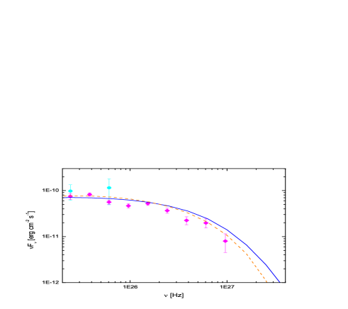
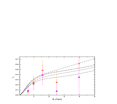
Figure 5: Left: Mrk 421 SED in low state in TeV window; The curves represent the TeV spectra calculated by LP model (solid line) and PLC model (dashed line). Right: Optical depth $\tau_{\gamma\gamma}$; The symbols represent $\tau_{\gamma\gamma}$ derived by using TeV spectra calculated by LP model (diamonds) and PLC model (circles); The curves represent $\tau_{\gamma\gamma}$ calculated by EBL model of Finke et al. (2008) (dashed), Franceschini et al. (2008) (dotted), Gilmore et al. (2012) (dash-double-dotted for WMAP5+fixed and short-dashed for fiducial WMAP5) and Kneiske, & Dole (2010) (dash-dotted).

4 Discussion and Conclusions

Using the MCMC method, we study the SED of Mrk 421 in different states for two kinds of EEDs with clear physical meanings: PLC and LP EEDs. Our results indicate that the EED in giant flare state is the LP shape and the stochastic turbulence acceleration is dominant, while in low activity the EED may be the PLC shape and the shock acceleration may play a more important role. This giant flare may be attributed to the re-acceleration of these electrons with PLC shape by stochastic process. Basically, we can understand this process from low state to flare state in the scenario proposed by Virtanen & Vainio (2005) that electrons injected at the shock front, then are accelerated at shock by Fermi I process and subsequently by the stochastic process in the downstream region. Here, we specify this scenario according to our results that the Fermi I process accelerated electrons are continuously injected into the emitting blob, and the SSC radiation from the steady EED (PLC shape) in the emitting blob is responsible for the emission of Mrk 421 in low state; Subsequently, the electrons with PLC shape are re-accelerated by stochastic process, and the EED with a significant curvature at high energies (LP) is formed, whose radiation contributes to the emission in flare state. A requirement in the scenario is that the magnetic field turbulence spectrum must be the case of the so-called “hard-sphere” approximation with the spectrum index $q=2$ since for cases of Kolmogorov turbulence ($q=5/3$) and Kraichna ($q=3/2$) turbulence, acceleration efficiency depend on the electron energy ($\gamma^{\prime}$), so that the acceleration efficiency for electrons with $\gamma^{\prime}\sim 10^{5}$ is very low and the escape would be dominant over the acceleration of electrons (e.g., Becker et al., 2006). This scenario including acceleration process also can account for the spectra hardening in flaring (e.g., Kirk et al., 1998). This scenario can be examined and the details of the flare can be studied in the time-dependent model. We will study them in the model including acceleration process (e.g., Kusunose et al., 2000; Katarzyński et al., 2006; Yan et al., 2012) in the coming work.

We notice that the jet of Mrk 421 appears to be particle dominated (see $U^{\prime}_{e}/U^{\prime}_{B}$ in Table 1,2), which is consistent with the result derived by Mankuzhiyil et al. (2011). Finally, we stress the caveat on EBL constraints we derived. The best-fit spectrum from optical through GeV is often extrapolated into TeV regime, and is considered as the intrinsic TeV spectrum. However, our results show that with different emission models, the best-fit SEDs from optical through GeV give different TeV spectra. Therefore, it should be considered in caution when such extrapolated TeV spectra is used to constrain the EBL models or redshift of source. The accurately measured VHE spectrum at E $>2$ TeV bands (e.g., Raue et al., 2012) could put more constraints on EBL models and emission models.

References

- Abdo et al. (2010) Abdo, A. A., Ackermann, M., Ajello, M., et al. 2010, ApJ, 710, 1271
- Abdo et al. (2011) Abdo, A. A., Ackermann, M., Ajello, M., et al. 2011, ApJ, 736, 131
- Ackermann et al. (2011) Ackermann, M., Ajello, M., Allafort, A., et al., 2011, ApJ, 743, 171
- Acciari et al. (2009) Acciari, V. A., Aliu, E., Aune, T. et al., 2009, ApJ, 703, 169
- Acciari et al. (2011) Acciari, V. A., Aliu, E., Aune, T. et al., 2011, ApJ, 738, 25
- Aharonian et al. (2009) Aharonian, F., Akhperjanian, A. G., Anton, G., et al., 2009, A&A, 502, 749
- Albert et al. (2007) Albert, J., Aliu, E., Anderhub, H. et al., 2007, ApJ, 663, 125
- Aleksić et al. (2010) Aleksić, J., Anderhub, H., Antonelli, L. A. et al., 2010, A&A, 519A, 32
- Bartoli et al. (2011) Bartoli, B., Bernardini, P., Bi, X. J. et al. 2011, ApJ, 734, 110
- Baring (1997) Baring, M. 1997, astro-ph/9711177
- Becker et al. (2006) Becker, P. A., Le, T., & Dermer, C. D. 2006, ApJ, 647, 53
- Błażejowski et al. (2005) Błażejowski, M., Blaylock, G., Bond, I. H. et al., 2005, ApJ, 630, 130
- Böttcher (2007) Böttcher, M. 2007, Ap&SS, 309, 95
- Böttcher & Dermer (2010) Böttcher, M., & Dermer, C. D. 2010, ApJ, 711, 445
- Chen et al. (2011) Chen, X., Fossati, G., Liang, E. P., Böttcher, M. 2011, MNRAS, 416, 2368
- Dermer & Schlickeiser (1993) Dermer, C. D., & Schlickeiser, R. 1993, ApJ, 416, 458
- Dermer et al. (2012) Dermer, C. D., Murase, K., Takami, H. 2012, ApJ, 755, 147
- Dimitrakoudis et al. (2012) Dimitrakoudis, S., Mastichiadis, A., Protheroe, R. J., Reimer, A. 2012, A&A, 546, A120
- Fan et al. (2010) Fan, Z. H., Liu, S. M., Yuan, Q., & Fletcher, L. 2010, A&A, 517, L4
- Finke et al. (2008) Finke, J. D., Dermer, C. D., & Böttcher, M. 2008, ApJ, 686, 181
- Finke et al. (2010) Finke, J. D., Razzaque, S., & Dermer, C D. 2010, ApJ, 712, 238
- Fossati et al. (2008) Fossati, G., Buckley, J. H., Bond, I. H. et al., 2008, ApJ, 677, 906
- Franceschini et al. (2008) Franceschini, A., Rodighiero, G., & Vaccari, M. 2008, A&A, 487, 837
- Galante et al. (2011) Galante, N., VERITAS Collaboration, arxiv:1109.6059
- Gamerman (1997) Gamerman, D. 1997, Markov Chain Monte Carlo: Stochastic Simulation for Bayesian Inference (Chapman and Hall, London)
- Garson et al. (2010) Garson, A. B., Baring, M. G., & Krawczynski, H. 2010, ApJ, 722, 358
- Gilmore et al. (2012) Gilmore, R. C., Somerville, R. S., Primack, J. R., Domínguez, A. 2012, MNRAS, 422, 3189
- Graff et al. (2008) Graff, P. B., Georganopoulos, M., Perlman, E. S., Kazanas, D. 2008, ApJ, 689, 68
- Kataoka et al. (2000) Kataoka, J., Takahashi, T., Makino, F., Inoue, S., Madejski, G. M., Tashiro, M., Urry, C. M., Kubo, H. 2000, ApJ, 528, 243
- Katarzyński et al. (2006) Katarzyński, K., Ghisellini, G., Mastichiadis, A., Tavecchio, F., Maraschi, L. 2006, A&A, 453, 47
- Katarzyński & Walczewska (2010) Katarzyński, K., & Walczewska, K. 2010, A&A, 510A, 63
- Kirk et al. (1998) Kirk, J. G., Rieger, F. M., & Mastichiadis, A. 1998, A&A, 333, 452
- Kneiske, & Dole (2010) Kneiske, T. M., & Dole, H. 2010, A&A, 515A, 19
- Kusunose et al. (2000) Kusunose, M., Takahara, F., Li, H., 2000, ApJ, 536, 299
- Lewis & Bridle (2002) Lewis, A., & Bridle, S. 2002, Phys. Rev. D, 66, 103511
- Liu et al. (2012) Liu, J., Yuan, Q., Bi, X. J., Li, H., and Zhang, X. M. 2012, PhRvD, 85, d3507 (arXiv:1106.3882)
- Mackay (2003) Mackay, D. J. C. 2003, Information Theory, Inference and Learning Algorithms (Cambridge University Press)
- Maraschi et al. (1992) Maraschi, L., Ghisellini, G., & Celotti, A. 1992, ApJL, 397, L5
- Mannheim (1993) Mannheim, K., 1993, A&A, 269, 67
- Massaro et al. (2004a) Massaro, E., Perri, M., Giommi, P., Nesci, R. 2004a, A&A, 413, 489
- Massaro et al. (2004b) Massaro, E., Perri, M., Giommi, P., Nesci, R., Verrecchia, F. 2004b, A&A, 422, 103
- Massaro et al. (2006) Massaro, E., Tramacere, A., Perri, M., Giommi, P., Tosti, G. 2006, A&A, 448, 861
- Massaro et al. (2011) Massaro, F., Paggi, A., & Cavaliere, A. 2011, ApJ, 742, L32
- Mankuzhiyil et al. (2010) Mankuzhiyil, N., Persic, M., & Tavecchio, F. 2010, ApJ, 715, L16
- Mankuzhiyil et al. (2011) Mankuzhiyil, N., Ansoldi, S., Persic, M., & Tavecchio, F. 2011, ApJ, 733, 14
- Mücke et al. (2003) Mücke, A., Protheroe, R. J., Engel, R. et al., 2003, APh, 18, 593
- Moraitis & Mastichiadis (2011) Moraitis, K. & Mastichiadis, A. 2011, A&A, 525A, 40
- Neal (1993) Neal, R. M. 1993, Probabilistic Inference Using Markov Chain Monte Carlo Methods (Department of Computer Science, University of Toronto)
- Punch et al. (1992) Punch, M., et al. 1992, Nature, 358, 477
- Ushio et al. (2010) Ushio, M., Stawarz, Ł., Takahashi, T. et la., 2010, ApJ, 724, 1509
- Raftery & Lewis (1992) Raftery, A. E., & Lewis, S. M. 1992, Stat. Sci., 7, 493
- Raue et al. (2012) Raue, M. et al., 2012, JPhCS, 355, 2001 (arxiv:1203.5956)
- Rees (1967) Rees, M. J. 1967, MNRAS, 137, 429
- Shukla et al. (2012) Shukla, A., Chitnis, V. R., Vishwanath, P. R. et al., 2012, A&A, 541A, 140
- Sikora et al. (1994) Sikora, M., Begelman, M. C., & Rees, M. J. 1994, ApJ, 421, 153
- Sokolov et al. (2004) Sokolov, A., Marscher, A. P., & McHardy, I. M. 2004, ApJ, 613, 725
- Stawarz & Petrosian (2008) Stawarz, L., & Petrosian, V. 2008, ApJ, 681, 1725
- Tavecchio et al. (1998) Tavecchio, F., Maraschi, L., Ghisellini, G., 1998, ApJ, 509, 608
- Tramacere et al. (2007) Tramacere, A., Massaro, F., Cavaliere, A. 2007, A&A, 466, 521
- Tramacere et al. (2009) Tramacere, A., Giommi, P., Perri, M., Verrecchia, F., Tosti, G. 2009, A&A, 501, 879
- Tramacere et al. (2011) Tramacere, A., Massaro, E., & Taylor, A. M. 2011, ApJ, 739, 66
- Virtanen & Vainio (2005) Virtanen, J., & Vainio, R. 2005, ApJ, 621, 313
- Yan et al. (2012) Yan, D. H., Zeng, H. D., & Zhang, L. 2012, MNRAS, 424, 2173