Cell Migration Model with Multiple Chemical Compasses

Abstract

A simple model is proposed that describes the various morphodynamic principles of migrating cells from polar to amoeboidal motions. The model equation is derived using competing internal cellular compass variables and symmetries of the system. Fixed points for the $N=2$ system are closely investigated to clarify how the competition among polaritors explains the observed morphodynamics. Response behaviors of cell–to–signal stimuli are also investigated. This model will be useful for classifying high-dimensional cell motions and investigating collective cellular behaviors.

The migration of cells on substrates is a key component of various biological functions, such as development, immune system response, and wound healing Bray . Cells exhibit diverse and involved morphodynamics depending on their type, developmental stage, and environmental conditions, and yet represent ordered and common dynamics across a range of species RidleySci2003 ; MoglinerCurrBiol2009 . Many cells exhibit an apparent monopolar shape, consisting of a head and a tail. The keratocyte-like crescent shape is also widely observed in nature KerenNat2008 . The highly investigated Dictyosterium cells form a roundish shape with amoeboidal, non-directed, random protrusions. Under poor nutrient conditions, these cells become elongated with a definitive polarity and exhibit a zig-zag (“split-and-choice”) motion AndrewNCB2007 ; Otsuji2010 , followed by a collective spiral migration pattern Sawai . These cellular behaviors are regulated by the cytoskeleton (specifically, actin filaments) mediated by signaling molecules (e.g., phosphoinositide lipids). It is now recognized that interactions among these molecules lead to the instability of a uniform molecular distribution inside a cell and generate self-organized chemical waves to support complex cell morphodynamic processes Vicker ; Gerisch ; Schoth-DiezHSFP2009 ; WeinerPLoSBiol2007 ; Arai20102012 ; Taniguchi . A number of theoretical models have been proposed by considering associated chemical reactions Otsuji2010 ; WeinerPLoSBiol2007 ; Arai20102012 ; Taniguchi ; Jinken ; Otsuji2007 ; Skpsky ; Shao ; Neilson2011 or actin polymerization Nishimura ; ShlomovitzPRL2007 ; Carlsson2010 ; DoubrovinskiPRL2011 ; EnculescuNJP2011 ; ZIebertJRSI2012 . However, these models are primarily focused on the onset of instabilities and a relatively simple pattern, and not generally intended to elucidate how a variety of morphodynamic processes from ordered to amoeboidal cell motions are organized. One of difficulties in addressing this issue is the requirement of large computational power for the execution of these models. Thus, simplified modeling with appropriate abstraction is another theoretical challenge in identifying the mechanism of diversity in cellular morphodynamics.

Here, we adopt one of the familiar concepts known as a “chemical compass,” which was introduced as a hypothetical internal cellular state and an intuitive representation of intrinsic cell directionality (Fig. 1(a)) RickertTCB2000 ; BourneNature2002 ; MeiliCell2003 ; SunBool2004 ; ArrieumerlouDevCell2005 ; KingTreCellBiol2009 . The compass can be interpreted to represent cellular polarity as dictated by molecular distribution. Based on the potential high dimensionality of molecular dynamics, there may be multiple cell compasses rather than only a single one. In practice, this is evident in amoeboidal motion, which exhibits a number of protrusions with patched molecular localization at the cell boundary (Fig. 1(b)). This is also supported by the observed mechanisms by which a cell responds to signal stimuli from different directions; cells turn by rotating their existing head in response to signals, although the existing head occasionally disappears in response to signals from the rear and a new head is formed in the direction of the signal (Fig. 1(c)) AndrewNCB2007 . These observations motivated us to introduce multiple compass variables for describing cellular dynamics. A model is derived in the following text for single cellular motion based on the competitive dynamics occurring among the hypothetical compass variables.

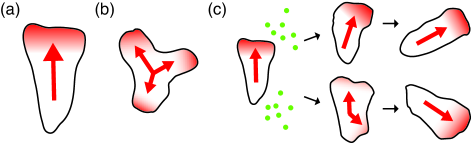
Figure 1: (a) Polarized cell represented by a single cellular compass variable (polaritor) (b) Amoeboidal cell represented by multiple polaritors. (c) Distinct responses to signal stimuli from different directions. The existing cell head turns in response to stimuli from the front to change direction (top), whereas the cell head is replaced by a new head in response to signals from the rear (bottom).

Intrinsic compass variables in the cell are represented by complex variables $W_{i}=R_{i}e^{{\rm i}\theta_{i}}(i=1,2,\ldots,N)$ with their amplitudes ($R_{i}$) and directions ($\theta_{i}$). We referr to the variables as polaritors in this study. A part of polaritors is supposed to be simultaneously active (i.e., $R_{i}>0$), while the other polaritors are in a quiescent state (i.e., $R_{i}=0$). The dynamics of these polaritors should satisfy the following requirements: First, a single polaritor spontaneously breaks U(1) symmetry, thereby obeying an equation similar to $\dot{W}=W-|W|^{m}W$ for an even integer $m$. Second, the system should satisfy all plausible symmetries; in other words, the equation should be invariant by the following transformation of variables: (i) simultaneous shift of polaritors’ direction $\theta_{i}\to\theta_{i}+\theta_{0}$ (isotropy), (ii) reflection $\theta_{i}\to-\theta_{i}$ for all $i$ (mirror symmetry), and (iii) permutation among polaritors’ indices. Third, the system should possess invariant subspaces specified by $W_{i}=0$ for each $i$, since polaritors in quiescent states should not influence the dynamics of the system. On the basis of these requirements, the following equation is proposed for the dynamics of $W_{i}$ Caption1 ;

$$\dot{W}_{i}\! = \!W_{i}\!-\!|W_{i}|^{4}W_{i}\!-\!\gamma\left(\Sigma^{\prime}|W_{j}|^{2}\right)W_{i}\!-\!\delta\left(\Sigma^{\prime}W_{j}^{2}\right)\overline{W}_{i}~{}~{}~{}$$ (1)

$$\!+~{}c_{1}\left(\Sigma^{\prime}W_{j}\right)|W_{i}|^{2}+c_{2}\left(\Sigma^{\prime}\overline{W}_{j}\right)W_{i}^{2}+\xi_{i}(t).$$

In this equation, $\overline{W_{i}}$ is the complex conjugate of $W_{i}$, $\Sigma^{\prime}\equiv\Sigma_{j\neq i}$ represents the calculation of the sum over $j$ except $i$, and the coefficients $\gamma,\delta,c_{1}$ and $c_{2}$ are real numbers due to the requirement of symmetry (ii). $m=4$ is adopted to ensure the stability of the system for arbitrary parameter values. The final term $\xi_{i}(t)$ is added to incorporate white Gaussian noise into the statistics $\langle\xi_{i}(t)\rangle=0$ and $\langle\xi_{i}(t)\xi_{j}(t^{\prime})\rangle=2D\delta_{ij}\delta(t-t^{\prime})/N$. In polar coordinates, Eq. (1), without the noise term, is expressed as

$$\dot{R}_{i}\! = \!R_{i}-R_{i}^{5}-\Sigma^{\prime}\left(\gamma+\delta\cos 2\!\left(\theta_{j}\!-\!\theta_{i}\right)\right)R_{j}^{2}R_{i}$$ (2)

$$\!+~{}\mu\Sigma^{\prime}\cos\left(\theta_{j}\!-\!\theta_{i}\right)R_{j}R_{i}^{2},$$

$$\dot{\theta}_{i}\! = \!-\delta\Sigma^{\prime}R_{j}^{2}\sin 2\!\left(\theta_{j}\!-\!\theta_{i}\right)+\nu\Sigma^{\prime}\sin\left(\theta_{j}\!-\!\theta_{i}\right)\!R_{j}R_{i}$$ (3)

where $\mu=c_{1}+c_{2}$ and $\nu=c_{1}-c_{2}$. These equations indicate that $\gamma$ represents angle-independent competition among polaritors, while $\delta$ and $\mu$ represent angle-dependent interactions of the first and second order. The velocity of the cell centroid $\bf{x}$ is set to obey the equation

$$\dot{\textbf{x}}=\textbf{v}=\sum{}_{i}W_{i}.$$ (4)

For visibility, the shape of the cell is assumed to depend on polaritors as an angular-radius function $L(\theta)=c^{-1}L_{0}(\theta)$ with $L_{0}(\theta)=\left(R_{0}+\sum_{i}R_{i}e^{\Lambda\cos(\theta-\theta_{i})}\right)$ and with the normalization factor $c^{2}=\frac{1}{2A}\int_{0}^{2\pi}\!\!L_{0}^{2}(\theta)d\theta$ to keep the cell area constant.

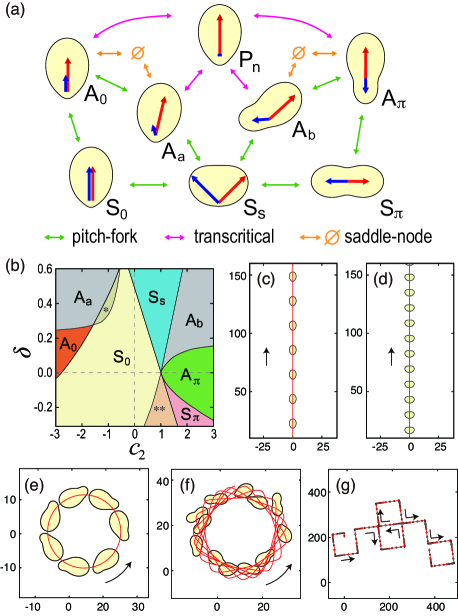
Figure 2: (a) Fixed points of the $N=2$ system and their relationship (see text). Red and blue arrows indicate polaritors. (b) Phase diagram of the $N=2$ system. $\gamma$ and $c_{1}$ are fixed as $\gamma=0.7$ and $c_{1}=1.0$. Different types of fixed points appear, depending on the initial condition in regions indicated by $\ast$ ($\bf{A_{0}}$ and $\bf{S_{0}}$) and $\ast\ast$ ($\bf{S_{0}}$ and $\bf{S_{\pi}}$). $\bf{P_{n}}$ may appear when $\gamma$ is sufficiently large ($\gamma>1+|\delta|$). (c-f) Examples of numerical simulations for the $N=2$ system. Red lines indicate the trajectories of cell centroids. Parameters $(\gamma,\delta,c_{1},c_{2})$ are set as (c) $(1.2,0.1,1.0,0.5)$, (d) $(0.7,0.4,1.0,1.0)$, (e) $(0.7,0.2,1.0,1.6)$, and (f) $(0.78,0.38,-0.45,0.45)$. Parameters for shape are set as $R_{0}=1.8$,$\Lambda=2.4$, and $A=0.3$.

To understand how the competition among polaritors gives rise to new dynamics, we first examined the simplest $N=2$ system in the absence of noise. With definitions of relative angle $\psi\equiv\theta_{2}-\theta_{1}$ and mean angle $\Psi\equiv(\theta_{1}+\theta_{2})/2$, Eqs. (2) and (3) reduce to

$$\dot{R}_{1}\! = \!R_{1}\!-\!R_{1}^{5}\!-\!\left(\gamma+\delta\cos 2\psi\right)\!R_{2}^{2}R_{1}+\mu\cos\psi R_{2}R_{1}^{2},~{}~{}~{}$$ (5)

$$\dot{R}_{2}\! = \!R_{2}\!-\!R_{2}^{5}\!-\!\left(\gamma+\delta\cos 2\psi\right)\!R_{1}^{2}R_{2}+\mu\cos\psi R_{1}R_{2}^{2},~{}~{}~{}$$ (6)

$$\dot{\psi}\! = \!\delta\left(R_{1}^{2}+R_{2}^{2}\right)\sin 2\psi-2\nu\sin\psi R_{1}R_{2},$$ (7)

$$\dot{\Psi}\! = \!\delta(R_{2}^{2}-R_{1}^{2})\sin 2\psi/2.$$ (8)

The equations for $R_{1},R_{2}$, and $\psi$ are incorporated within these variables; $\Psi$ evolves depending on these variables, and thus, the dynamics related to $(R_{1},R_{2},\psi)$ is the primary interest herein. The domain of $\psi$ can be restricted to $-\pi\!<\!\psi\!\leq\!\pi$. We observed that a variety of fixed points appear in this system (Fig. 2(a)) as listed below, where several obvious fixed points obtained by replacing $i=1$ and $2$ are excluded. The stability of these fixed points are also determined by considering the linear equation $\dot{\vec{\rho}}=J\vec{\rho}$, where $\vec{\rho}$ indicates a small deviation in $(R_{1},R_{2},\psi)$ and $J$ is a Jacobian matrix at a fixed point. Eigenvalues and corresponding eigenvectors of $J$ are denoted as $\lambda\!=\!(\lambda_{1},\lambda_{2},\lambda_{2})$ and $\vec{\rho}_{1},\vec{\rho}_{2},\vec{\rho}_{3}$, respectively. Fig. 2(a) summarizes the fixed points and their relationships.

[$\bf{Z}$] $(R_{1},R_{2})=(0,0)$ for arbitrary $\psi$. This is a trivial fixed point with $\lambda_{1}=\lambda_{2}=1$ and $\lambda_{3}=0$, and always remains unstable.

[$\bf{P_{n}}$] $(R_{1},R_{2},\psi)=(1,0,n\pi/2)$ with $n$ as an integer (Fig. 2(a)). These fixed points are also an expected trivial state, where one polaritor is active while the other is quiescent. Eigenvalues are denoted as $\lambda_{1}=-4,\lambda_{2}=1-(\gamma+\delta\cos 2\psi)$, and $\lambda_{3}=2\delta\cos 2\psi$. One of these fixed points is stable as long as $\gamma>1+|\delta|$.

[$\bf{S_{0}},\bf{S_{\pi}},\bf{S_{s}}$] Fixed points with symmetric finite amplitudes ($R_{1}\!=\!R_{2}\!=R\!>\!0$; Fig. 2(a)). Directions of the two polaritors coincide for $\rm{\bf S_{0}}$ ($\psi\!=\!0$), but are reversed for $\rm{\bf S_{\pi}}$ ($\psi\!=\!\pi$). $\rm{\bf S_{s}}$ has a non-trivial relative angle $\psi_{s}$ that is determined by $\cos\psi_{s}=\nu/2\delta$. Square amplitudes $R_{0}$, $R_{\pi}$, and $R_{s}$ are defined by $R^{2}=[-(\gamma+\delta\cos 2\psi-\mu\cos\psi)+\sqrt{(\gamma+\delta\cos 2\psi-\mu\cos\psi)^{2}+4}]/2$ with the substitution of $\psi=0$, $\pi$, and $\psi_{s}$, respectively. The linear stability of these fixed points are evaluated by $\lambda_{1}=2-6R^{4}$, $\lambda_{2}=-2-2R^{4}$, and $\lambda_{3}=2R(2\delta\cos 2\psi-\nu\cos\psi)$. The eigenvector of $\lambda_{3}$ is $\vec{\rho}_{3}=(0,0,1)$, indicating that $\lambda_{3}$ defines stability in the direction of the relative angle $\psi$ (angular stability). $\rm{\bf S_{0}}$ and $\rm{\bf S_{\pi}}$ are unstable in the angular direction in the regions $\nu<2\delta$ and $\nu>-2\delta$, respectively, in which $\rm{\bf S_{s}}$ appears through pitch-fork bifurcation. In contrast, $\lambda_{1}$ has the eigenvector $\vec{\rho}_{1}=(1,-1,0)$ and defines stability in the amplitudal directions; $\lambda_{1}>0$ indicates a break in the amplitudal symmetry. $\lambda_{2}$ is always negative and does not alter stability.

[$\bf{A_{0}}$] Fixed points at which two polaritors have distinct finite amplitudes and the same direction ($R_{1}\!>\!R_{2}\!>\!0$ and $\psi\!=\!0$; Fig. 2(a)). The condition of the fixed points is defined by $R_{1}^{2}\!+\!R_{2}^{2}\!\!=\!\gamma\!+\!\delta$ and $R_{1}^{4}\!+\!R_{2}^{4}\!+\!\left(\gamma\!+\!\delta\right)^{2}\!=\!2\mu R_{1}R_{2}$ (see Eqs. ​​(5-7)). Two types of solutions appear as a pair of saddle-node bifurcations at $4(\gamma+\delta)^{2}\!+\!\mu^{2}\!=\!4$. One of them is always unstable, irrespective of parameter values, and is never realized. Only the other fixed point, denoted as $\rm{\bf{A_{0}}}$, can be realized. By denoting $\gamma^{\prime}\!\equiv\!\gamma\!+\!\delta$, square amplitudes of the solution are defined as $R_{1}^{2}\!=\![\gamma^{\prime}+\!\{\gamma^{\prime 2}-\!(-\mu-\!\sqrt{\mu^{2}\!+\!4\gamma^{\prime 2}\!-\!4})^{2}\}^{1/2}]/2$ and $R_{2}^{2}\!=\![\gamma^{\prime}-\!\{\gamma^{\prime 2}-\!(-\mu-\!\sqrt{\mu^{2}\!+\!4\gamma^{\prime 2}\!-\!4})^{2}\}^{1/2}]/2$. Through the change in the amplitudal direction, this fixed point connects to $\rm{\bf S_{0}}$ via pitch-fork bifurcation and connects to $\rm{\bf P_{n}}$ via transcritical bifurcation (Fig. 2(a)). Angular stability is lost when the eigenvalue $\lambda_{3}\!=\!2\gamma^{\prime}\delta\!-\!2\nu R_{1}R_{2}$ is positive, with an eigenvector of $\vec{\rho}_{3}\!=\!(0,0,1)$.

[$\bf{A_{\pi}}$] Fixed points at which two polaritors have distinct, finite amplitudes and opposite directions ($R_{1}\!>\!R_{2}\!>\!0$ and $\psi\!=\!\pi$; Fig. 2(a)). Similar to the case of $\rm{\bf A_{0}}$, two types of fixed points appear as a pair of saddle-node bifurcations at $4\gamma^{\prime 2}\!+\!\mu^{2}\!=\!4$. One of these points is always unstable, and only the other, $\rm{\bf A_{\pi}}$, can be realized. The solution relates $\rm{\bf S_{\pi}}$ and $\rm{\bf P_{n}}$ via pitch-fork and transcritical bifurcations, respectively (Fig. 2(a)). Angular stability is lost when $\lambda_{3}\!=\!2\delta(\gamma+\!\delta)\!+\!2\nu R_{1}R_{2}$ is positive. Square amplitudes at $\rm{\bf A_{\pi}}$ are defined as $R_{1}^{2}\!=\![\gamma^{\prime}+\!\{\gamma^{\prime 2}-\!(\mu-\!\sqrt{\mu^{2}\!+\!4\gamma^{\prime 2}\!-\!4})^{2}\}^{1/2}]/2$ and $R_{2}^{2}\!=\![\gamma^{\prime}-\!\{\gamma^{\prime 2}-\!(\mu-\!\sqrt{\mu^{2}\!+\!4\gamma^{\prime 2}\!-\!4})^{2}\}^{1/2}]/2$.

[$\bf{A_{a},A_{b}}$] Fixed points with distinct, finite amplitudes ($R_{1}\!>\!R_{2}\!>\!0$) and a $\psi$ that is neither $0$ nor $\pi$ (Fig. 2(a). These solutions are obtained from the following conditions derived from Eqs. (5-7): $R_{1}^{2}+R_{2}^{2}=\gamma+\delta\cos 2\psi$, $R_{1}^{4}+R_{2}^{4}+\left(\gamma+\delta\cos 2\psi\right)^{2}=2\mu\cos\psi R_{1}R_{2}$, and $\delta\left(R_{1}^{2}+R_{2}^{2}\right)\cos\psi=\nu R_{1}R_{2}$. The expression giving the solutions is lengthy and of secondary importance for the purpose of this work. We showed that there can be twelve types of possible solutions. Two of them bifurcate from $\rm{\bf A_{0}}$ and $\rm{\bf A_{\pi}}$ by the angular instabilities through pitch-fork bifurcations. Let us denote them as $\rm{\bf A_{a}}$ and $\rm{\bf A_{b}}$, respectively. These two fixed points are separated, since $R_{1}\!=\!R_{2}\!=\!0$ at $\psi\!=\!\pm\pi/2$; $|\psi|$ is less than $\pi/2$ for $\rm{\bf A_{a}}$ but larger than $\pi/2$ for $\rm{\bf A_{b}}$. The other fixed points are mostly unstable; two of them may appear in the limited parameter regions via saddle-node or subcritical bifurcation (these fixed points are not discussed further in this report).

Figure 2(b) shows the phase diagram against $c_{2}=(\mu-\nu)/2$ and $\delta$, with fixed values of $\gamma=0.7$ and $c_{2}=1.0$. At the fixed points $\rm{\bf P_{n}}$, $\rm{\bf S_{0}}$, $\rm{\bf S_{s}}$, $\rm{\bf A_{0}}$, and $\rm{\bf A_{\pi}}$, cells move directionally straight ($\dot{\Psi}=0$), but they have different shapes. Examples of cell motion at $\rm{\bf P_{n}}$ and $\rm{\bf S_{s}}$ are shown in Fig. 2(c) and (d), which are similar to polarized and keratocyte-like cell motions, respectively. On the other hand, $\dot{\Psi}$ is nonzero and the cells show migration with a circular orbit at the fixed points $\rm{\bf A_{a}}$ and $\rm{\bf A_{b}}$ (Fig. 2(e)). A cell at fixed point $\rm{\bf S_{\pi}}$ is bipolar and does not exhibit migration.

In addition to these fixed points, numerical simulations revealed oscillatory dynamics in narrow parameter regions Caption2 . The cell in the oscillatory state exhibits a quasi-periodic Lissajous orbit, as shown in Fig. 2 (f). Another type of motion found by numerical simulation is repetitive right angle turns (Fig. 2(g)). Similar types of motions were reported for another model HiraiwaEPL2010 .

Taken together, many inner states appear on account of the competition among polaritors, even in the simplest system of $N=2$. Note that Eq. (7) indicates that $\psi=0$ and $\psi=\pi$ are separatrices in the phase space of the $N=2$ system. In addition, $r\equiv R_{2}-R_{2}$ obeys the equation of the form $dr/dt=Q\times r$ from Eqs. (5) and (6), where $Q$ is a function of $(R_{1},R_{2},\psi)$, indicating that $R_{1}=R_{2}$ is an additional separatrix in the system. Thus, the order in amplitudes of polaritors defined by the initial condition is maintained in a noiseless system. These separatrices constrain the dynamics of the $N=2$ system; for example, zig-zag motion is forbidden.

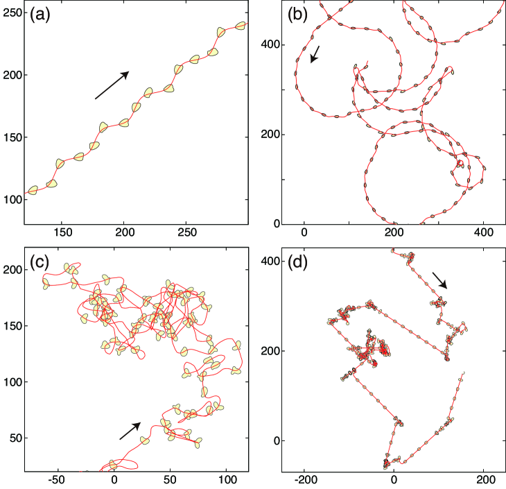
Figure 3: (a) Zig-zag motion for the $N=3$ system with parameters $(\gamma,\delta,c_{1},c_{2})=(0.78,0.3,0.6,0.8)$. (b) Chaotic motion for the $N=3$ system. Parameters are set as $(0.8,0.55,0.35,-0.8)$. (c,d) Examples of chaotic motions in the $N=20$ systems. Parameters are set as $(0.7,0.3,0.6,0.8)$ (c) and $(1.2,-0.22,0.8,2.35)$ (d). Parameters for shapes are set as $(R_{0},\Lambda,A)=(1.5,12.0,0.3)$ for (a,b) and $(1.8,4.0,0.3)$ for (c,d).

Such constraints are absent for $N>2$; therefore, the system can exhibit various types of motion. For $N=3$, zig-zag motion of cell migration is observed, as shown in Fig. 3(a), where two oscillating polaritors dictate the position of the head of the cell and periodically determine the direction of migration. Chaotic inner dynamics is found in the case where the cellular trajectory is also a chaotic orbit, as shown in Fig. 3(b). For larger $N$ systems, additional types of dynamics appear. Fig. 3(c) shows an example of cellular motion at the $N=20$ system, wherein the cell shape can fluctuate significantly, similar to the case of amoebic motion. Fig. 3(d) shows another example in the $N=20$ system, for which the cell exhibits repetitively straight motion, followed by locally diffusive random migration.

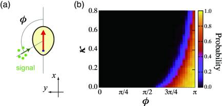
Figure 4: (a) Set-up of the numerical simulation. A cell with a polaritor directed in the $x$-direction receives a signal from direction $\phi$ at $t=0$. (b) Probability of cell directional change by the replacement of polaritors is shown in a color scale against the invoked signal direction $\psi$ and parameter $\kappa$. The replacement can occur only when $\phi>\pi/2$. Parameters are set as $\gamma=1.4$, $\delta=0.15$, $\mu=0.3$, $\nu=-0.1$, $\sigma=2.0$, and $s=1.0$. A small amount of noise is added during the simulation ($D=5.0\times 10^{-3}$). The probability is calculated from 100 independent simulations for each parameter set.

Finally, we considered the chemotactic behavior of a cell in a signal field $S(\mbox{{x}},t)$ Devreotes2003 ; VanHaastert2004 . Cell shapes and internal cellular compasses are correlated with the sensing ability to external signal molecules. Assuming that a cell can sense the gradient of the signal field $s(\textbf{x})\equiv\nabla S(\textbf{x})=s(\textbf{x})e^{i\phi(\textbf{x})}$, the coupling of polaritor variables with the signal field is incorporated by combining $d_{1}s|W_{i}|^{2}+d_{2}\overline{s}W^{2}_{i}$ with Eq. (1). For $\sigma=d_{1}+d_{2}$ and $\kappa=d_{1}-d_{2}$, the following additional terms appear in Eqs. (2) and (3):

$$\dot{R}^{sig}_{i} = \sigma sR^{2}_{i}\cos(\theta_{i}-\phi),$$ (9)

$$\dot{\theta}^{sig}_{i} = \kappa sR_{i}\sin(\phi-\theta_{i}).$$ (10)

Here, both $\sigma$ and $\kappa$ are set as positive for an attractant signal. For a single polaritor with $R\sim 1$, the direction develops as $\dot{\theta}_{i}\sim\kappa s\sin(\phi-\theta_{i})$ and is directed to the maximum gradient of the signal concentration, as introduced previously HuPRE2010 . When $|\theta_{i}-\phi|$ is larger than $\pi/2$, $\dot{R}_{i}^{sig}$ becomes negative and the existing polaritor begins to shrink. Thus, the replacement of polaritors may occur, depending on the direction of the signal gradient.

To confirm the response of cellular behaviors, numerical simulation is conducted with the following settings. First, a cell with $N=2$ polaritors at the single polarity state $\bf{P_{n}}$ is prepared in the absence of a signal field. The active polaritor is set in the $x$-direction. Then, a signal field is applied at $t=0$ with $\textbf{s}(t)=se^{i\phi}\Theta(t)$, where $s$ and $\phi$ are constants and $\Theta(\cdot)$ is a Heaviside function (Fig. 4(a)). Weak noise is added ($D=5.0\times 10^{-3}$). Then, the system shows either rotation of the existing polaritor (Fig. 1(c), top) or the replacement of polaritors (bottom), depending on signal direction $\phi$ and other parameters. Fig. 4(b) shows the probability of the replacement occurring for respective signal direction $\psi$ and parameter $\kappa$. The results demonstrate that the model cell can respond to signal stimuli from the rear ($\phi>\pi/2$) by switching polaritors.

By considering competition among polaritors, the present study investigates a mechanism for organizing a variety of cellular behaviors linked to morphology and migration. The proposed model exhibits distinct polar, keratocyte-like, zig-zag, and chaotic amoeboid motions that are relevant to experimental observations. This model is only constrained by the symmetry of the system. As demonstrated in different systems like quadrupedal locomotion Golubitsky , such an approach based on symmetry can be helpful in classifying a variety of possible cellular motions. In addition, the model is quite simple and requires little computational power, making it possible to use the model to study collective cellular behaviors Vicsek ; LevinePRE2001 .

An advantage of our model is that it is easily extensible to higher dimensions even with the same number of model parameters, and it provides an intuitive and consistent interpretation of cellular behavior. Previous models have been reported Ohta_PRL2009 ; HiraiwaEPL2010 that exhibit similar dynamics to those presented in this study. However, these models become complicated by including higher-order tensor variables; in fact, zig-zag and chaotic motions appear in the equations that contain more than 20 parameters HiraiwaEPL2010 .

Because the concept of a polaritor is introduced here as a rather abstract variable, a future step will be to identify the molecular basis of the polaritors and their interactions. Validating Eq. (1) from detailed subcellular processes (e.g., reduction from detailed models Otsuji2010 ; WeinerPLoSBiol2007 ; Arai20102012 ; Taniguchi ; Jinken ; Otsuji2007 ; Skpsky ; Shao ; Neilson2011 ; Nishimura ; ShlomovitzPRL2007 ; Carlsson2010 ; DoubrovinskiPRL2011 ; EnculescuNJP2011 ; ZIebertJRSI2012 ) will elucidate the way in which cellular motion depends on molecular parameters, which improves the correspondence of the model with experimental observations.

The author thanks D. Taniguchi, A. Nakajima, S. Sawai, and K. Kaneko for the valuable comments. This work was supported by the Grant-in-Aid MEXT/JSPS (No. 24115503).

References

- (1) D. Bray, Cell Movements: From Molecules to Motility, 2nd ed. (Garland, New York, 2001)
- (2) A.J. Ridley et al., Science 302, 1704 (2003)
- (3) A. Mogilner and K. Keren, Curr. Biol. 19, R762 (2009)
- (4) K. Keren, et al. Nature 453, 475 (2008)
- (5) N. Andrew and R.H. Insall, Nat. Cell Biol. 9, 193 (2007)
- (6) M. Otsuji, Y. Terashima, S. Ishihara, S. Kuroda, and K. Matsushima, Sci. Sig. 3(152):ra89 (2010)
- (7) S. Sawai, P.A. Thomason, and E.C. Cox, Nature 433, 323 (2005)
- (8) M. Vicker, FEBS Lett. 510, 5 (2002)
- (9) T. Bretschneider, et al., Curr. Biol. 14,1 (2004); T. Bretschneider, et al., Biophys. J. 9, 2888 (2009);
- (10) G. Gerisch, et al. Biophys. J. 87, 3493 (2004); B. Schroth-Diez, et al. HFSP J. 3, 412 (2009); G. Gerisch, et al. Cell Adh. Migr. 3, 373 (2009); G. Gerisch, B. Schroth-Diez, A. Müller-Taubenberger, and M. Ecke, BioPhys. J. 103, 1170 (2012)
- (11) O.D. Weiner, W.A. Marganski, L.F. Wu, S.J. Altschuler, and M.W. Kirschner, PLoS Biol. 5, e221 (2007)
- (12) Y. Arai, T. Shibata, S. Matsuoka, M.J. Sato, T. Yanagida, and M. Ueda, Proc. Natl. Acad. Sci. USA 107, 12399 (2010); T. Shibata, M. Nishikawa, S. Matsuoka, and M. Ueda, J. Cell Sci. doi: 10.1242/jcs.108373 (2012)
- (13) D. Taniguchi, S. Ishihara, T. Oonuki, M. Honda, K. Kaneko, and S. Sawai, under revision.
- (14) A. Jilkine and L. Edelstein-Keshet, PLoS Comput. Biol. 7, e1001121 (2011)
- (15) M. Otsuji, S. Ishihara, C. Co, K. Kaibuchi, A. Mochizuki, and S. Kuroda, PLoS Comput. Biol. 3, e108 (2007)
- (16) R. Skupsky, W. Losert, and R.J. Nossal, Biophys. J. 89, 2806 (2005)
- (17) D. Shao, W.-J. Rappel, and H. Levine, Phys. Rev. Lett. 105 108104 (2010); D. Shao, H. Levine, and W.-J. Rappel, Proc. Natl. Acad. Sci. USA 109, 6851 (2012)
- (18) M.P. Neilson, D.M. Veltman, P.J.M. Van Haastert, S.D. Webb, J.A. Mackenzie, and R.H. Insall, PLoS Biol. 9, e1000618 (2011)
- (19) S.I. Nishimura and M. Sasai, J. Theor. Biol. 245, 230 (2007); S.I. Nishimura, M. Ueda, and M. Sasai, Phys. Rev. E 85, 041909 (2012)
- (20) R. Shlomovitz and N.S. Gov, Phys. Rev. Lett. 98, 168103 (2007)
- (21) A.E. Carlsson, Phys. Rev. Lett. 104, 228102 (2010)
- (22) K. Doubrovinski and K. Kruse, Phys. Rev. Lett. 107, 258103 (2011)
- (23) M. Enculescu and M. Falcke, New J. Phys. 13, 053040 (2011)
- (24) F. Ziebert, S. Swaminathan, and I.S. Aranson, J. Royal Soc. Interface 9, 1084 (2012)
- (25) T. Ohta and T. Ohkuma, Phys. Rev. Lett. 102, 154101 (2009)
- (26) T. Hiraiwa, M.Y. Matsuo, T. Ohkuma, T. Ohta, and M. Sano, Eur. Phy. Lett. 91, 20001 (2010)
- (27) P. Rickert, O.D. Weiner, F. Wang, H.R. Bourne, and Guy Servant, Trends Cell. Biol. 10, 466 (2000)
- (28) H.R. Bourne and O. Weiner, Nature 419, 21 (2002)
- (29) R. Meili and R.A. Firtel, Cell 114, 153 (2003)
- (30) C.X. Sun, G.P. Downey, F. Zhu, A.L.Y. Koh, H. Thang, and M. Glogauer, Blood 104, 3758 (2004).
- (31) C. Arrieumerlou and T. Meyer, Dev. Cell 8, 215 (2005)
- (32) J.S. King and R.H. Insall, Trends Cell Biol. 19, 523, (2009)
- (33) Interaction terms among three polaritors like are ignored.
- (34) No chaotic motion is found in the system.
- (35) P. Devreotes and C. Janetopoulos, J. Biol. Chem. 278, 20445 (2003)
- (36) P.J. Van Haastert and P.N. Devreotes, Nat. Rev. Mol. Cell Biol. 5, 626 (2004).
- (37) B. Hu, D. Fuller, W.F. Loomis, H. Levine, and W.-J. Rappel, Phys. Rev. E 81, 031906 (2010)
- (38) M. Golubitsky and I. Stewart, The Symmetry Perspective: From Equilibrium to Chaos in Phase Space and Physical Space, (Birkhauser, 2003)
- (39) T. Vicsek, A. Czirók, E. Ben-Jacob, I. Cohen and O. Shochet, Phys. Rev. Lett. 75, 1226 (1995)
- (40) H. Levine, W.-J. Rappel and I. Cohen, Phys. Rev. E 63, 017101 (2001)