It is general knowledge that the harmonic mean and that the geometric mean , where and are two positive numbers. In the paper, the authors show by several approaches that the harmonic mean and the geometric mean are all Bernstein functions of and establish integral representations of the means and .
Key words and phrases:
Bernstein function; Harmonic mean; Geometric mean; Integral representation; Stieltjes function; induction; Cauchy integral formula; Stieltjes-Perron inversion formula
If for some nonnegative integer is completely monotonic on an interval , but is not completely monotonic on , then is called a completely monotonic function of -th order on an interval .
Let be a nonnegative function and have derivatives of all orders on . A number is said to be the completely monotonic degree of with respect to if is a completely monotonic function on but is not for any positive number .
In what follows, for convenience, we denote the sets of completely monotonic functions on , logarithmically completely monotonic functions on , Stieltjes functions, and Bernstein functions on by , , , and respectively.
1.2. Some relationships and a characterization
Now we briefly describe some basic relationships between the above defined classes of functions and list a characterization of Bernstein functions on .
In [3, 10, 20, 22], any logarithmically completely monotonic function on an interval was once again proved to be completely monotonic on . In [3], the set of all Stieltjes functions was proved to be a subset of all logarithmically completely monotonic functions on . See also [24, Remark 4.8]. Conclusively,
(1.4)
It is obvious that any nonnegative completely monotonic function of first order is a Bernstein function.
The relation between Bernstein functions and logarithmically completely monotonic functions was discovered in [7, pp. 161–162, Theorem 3] and [25, p. 45, Proposition 5.17], which reads that the reciprocal of any positive Bernstein function is logarithmically completely monotonic. In other words,
(1.5)
A relation between and was given by [4, Theorem 5.4] which may be recited as
(1.6)
It is easy to see that the degree of any completely monotonic function on is at least zero. Conversely, if a nonnegative function on has a nonnegative degree , then it must be a completely monotonic function on . See [9, p. 9890].
Bernstein functions can be characterized by [25, p. 15, Theorem 3.2] which states that a function is a Bernstein function if and only if it admits the representation
(1.7)
where and is a measure on satisfying
For information on characterizations of the classes and , please refer to related texts in [3, 25, 27] and references cited therein.
1.3. Some means
We recall from [26] that the extended mean value may be defined by
(1.8)
(1.9)
(1.10)
(1.11)
where are positive numbers and . Because this mean was first defined in [26], so it is also called Stolarsky’s mean by a number of mathematicians. Many special means with two positive variables are special cases of , for example,
For more information on , please refer to the monograph [6], the papers [11, 12, 19, 13], and a lot of closely-related references therein.
1.4. The arithmetic mean is a Bernstein function
It is easy to see that the arithmetic mean
is a trivial Bernstein function of for .
1.5. The exponential mean is a Bernstein function
In [23, p. 116, Remark 6], it was pointed out that,
(1)
by standard arguments, it is easy to verify that the reciprocal of the exponential mean
(1.12)
for with is a logarithmically completely monotonic function of ;
(2)
from the newly-discovered integral representation
(1.13)
it is easy to obtain that the exponential mean for with is also a completely monotonic function of first order (that is, a Bernstein function).
was proved to be increasing and concave in for with .
More strongly, the logarithmic mean was proved in [21, Theorem 1] to be a completely monotonic function of first order on for with . Therefore, the logarithmic mean is a Bernstein function of .
Remark 1.1.
By [7, pp. 161–162, Theorem 3] or [25, p. 45, Proposition 5.17], the logarithmically complete monotonicity of the exponential mean and the logarithmic mean can be deduced respectively from their common property that they are Bernstein functions.
1.7. Main results
The goals of this paper are to prove that the harmonic mean
(1.15)
and the geometric mean
(1.16)
are all Bernstein functions of on for with , and to establish integral representations of and .
2. Lemmas
In order to prove our main results, the following lemmas are needed.
Lemma 2.1.
For , the -th derivatives of the functions
(2.1)
the reciprocal , and
(2.2)
on may be computed by
(2.3)
(2.4)
(2.5)
where
(2.6)
(2.7)
(2.8)
Consequently, the functions and are completely monotonic on , and the reciprocal is a Bernstein function on .
for . It is easy to verify that the sequence (2.31) for meets the recursion formulas (2.10), (2.11), and (2.12). The formulas (2.3) and (2.6) for general terms are thus proved.
It is obvious that
which is equivalent to
Therefore, using the formulas (2.3) and (2.6) just verified, we have
Hence, the general formulas (2.4) and (2.7) are obtained.
In [25, p. 13, Remark 2.4], it was collected as an example that the function is a Stieltjes function for . The property (iv) in Section 3 of [4] (See also the property (vii) in [16, Theorem 1.3]) reads that if then for . Specially for and , we have . The property (i) in Section 3 of [4] (See also the property (i) in [16, Theorem 1.3]) states that if then . Applying this property to brings out
(2.32)
which means, by the relation from the very ends of the inclusions (1.4), that and, by the relation (1.6), that .
In [25, p. 24, Remark 3.11], it was listed as examples that for and . The item (iii) of Corollary 3.7 in [25, p. 20] write that if then . Applying and respectively to and reveals once again that .
Taking and . It is easy to see that and . A part of Theorem 3.6 in [25, p. 19] asserts that if then for every . Since , applying and in this assertion respectively to and leads to . The proof of Lemma 2.1 is completed.
∎
Lemma 2.2.
For , the complex functions and have integral representations
(2.33)
and
(2.34)
Consequently, the functions and are Stieltjes functions and the complex function has the integral integral representation
(2.35)
for , where
(2.36)
is nonnegative on and
(2.37)
on .
Proof by Cauchy integral formula.
By standard arguments, we immediately obtain that
(2.38)
(2.39)
(2.40)
(2.41)
(2.42)
(2.43)
For and , we have
where
Hence,
Accordingly,
(2.44)
Similarly, for and , we have
Therefore,
Consequently,
(2.45)
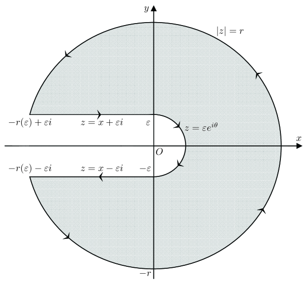
Let be a bounded domain with piecewise smooth boundary. The famous Cauchy integral formula (See [8, p. 113]) reads that if is analytic on , and extends smoothly to the boundary of , then
(2.46)
For any fixed point , choose and such that , and consider the positively oriented contour in consisting of the half circle for and the half lines for until they cut the circle , which close the contour at the points , where as . See Figure 1.
Figure 1. The contour
By the above mentioned Cauchy integral formula, we have
The property (x) in [16, Theorem 1.3] formulates that if then for .
Since , see (2.32), and, by the property (i) in [16, Theorem 1.3], , replacing by , making use of the easy fact that , and letting yield .
For a Stieltjes function given by (1.3), by the Stieltjes-Perron inversion formula in [14, p. 591], we can determine the scalars and and the measure
(2.55)
as done in [3, 15]. Specially, for the function , since and , we have
(2.56)
for , where
when and when because taking we obtain
when and when . Thus we find
when and when . Substituting in the representation (2.56) results in the formula (2.33).
The formula (2.34) for or for can be derived in a similar way as above.
The rest is the same as in the first proof. Lemma 2.2 is proved once again.
∎
3. The harmonic mean is a Bernstein function
Our results on the harmonic mean may be stated as the theorem below.
Theorem 3.1.
The harmonic mean defined by (1.15) is a Bernstein function of on for with and has the integral representation
(3.1)
Consequently,
(3.2)
(3.3)
Proof.
The harmonic mean meets
(3.4)
It is obvious that the derivative is completely monotonic with respect to . As a result, the harmonic mean is a Bernstein function of on for with .
In [1, p. 255, 6.1.1], it was listed that, for and , the classical Euler gamma function
and so, by integrating with respect to on both sides of (3.7), the formula (3.1) follows.
Letting on both sides of (3.1) and using the limit
generate the formula (3.2).
Taking in (3.1) produces (3.3). Theorem 3.1 is thus proved.
∎
Remark 3.1.
By [7, pp. 161–162, Theorem 3] or [25, p. 45, Proposition 5.17], it can be derived that the reciprocal of the harmonic mean , that is, the function , is logarithmically completely monotonic.
This logarithmically complete monotonicity can also be proved by considering
and that the product and sum of finitely many completely monotonic functions are also completely monotonic functions.
Moreover, from (3.4), it follows readily that is an increasing function in for with .
4. The geometric mean is a Bernstein function
Our results on the geometric mean can be summarized as two theorems.
Theorem 4.1.
Let with . Then the geometric mean defined by (1.16) is a Bernstein function of on .
This means that the derivative is logarithmically completely monotonic, and so it is also completely monotonic. As a result, the geometric mean is a Bernstein function.
∎
Second proof.
It is clear that the geometric mean satisfies
(4.3)
and
(4.4)
where
(4.5)
If , then for and is completely monotonic in . On the other hand, the function is positive and
for , which implies that the function is completely monotonic on ; A ready modification of a conclusion in [5, p. 83] yields the following conclusion: If and are completely monotonic functions such that is defined on an interval , then is also completely monotonic on ; So, when , the derivative is completely monotonic and the geometric mean is a Bernstein function. Consequently, considering the symmetric property , it is easily obtained that the geometric mean for with is a Bernstein function.
∎
Remark 4.1.
From the equality in (4.3), it is easy to derive that the function is increasing in for with .
From (4.4), it is immediate to deduce that the reciprocal of the geometric mean is a logarithmically completely monotonic function of for with .
which means that, when , the derivative is completely monotonic. Since , when , the derivative is also completely monotonic. This implies that the geometric mean is a Bernstein function of .
∎
Theorem 4.2.
For and , the geometric mean has the integral representation
(4.7)
where the function is defined by (2.36). Consequently, the geometric mean is a Bernstein function of on .
Integrating with respect to from to on both sides of the above equation and interchanging the order of integrals yield
Since , the integral representation (4.7) is readily deduced.
By the characterization expressed by (1.7) and the integral representation (4.7) applied to , it is immediate to see that the geometric mean is a Bernstein function of on .
∎
The equality in (4.8) is valid if and only if . This gives a new proof of the fundamental and well known AG mean inequality.
References
[1]
M. Abramowitz and I. A. Stegun (Eds), Handbook of Mathematical Functions with Formulas, Graphs, and Mathematical Tables, National Bureau of Standards, Applied Mathematics Series 55, 9th printing, Washington, 1970.
[2]
R. D. Atanassov and U. V. Tsoukrovski, Some properties of a class of logarithmically completely monotonic functions, C. R. Acad. Bulgare Sci. 41 (1988), no. 2, 21–23.
[3]
C. Berg, Integral representation of some functions related to the gamma function, Mediterr. J. Math. 1 (2004), no. 4, 433–439.
[4]
C. Berg, Stieltjes-Pick-Bernstein-Schoenberg and their connection to complete monotonicity, In: Positive Definite Functions. From Schoenberg to Space-Time Challenges, S. Mateu and E. Porcu (eds.), Dept. Math., Univ. Jaume I, Castellón de la Plana, Spain, 2008, 24 pages.
[5]
S. Bochner, Harmonic Analysis and the Theory of Probability, University of California Press, Berkeley-Los Angeles, 1960.
[6]
P. S. Bullen, Handbook of Means and Their Inequalities, Mathematics and its Applications, Volume 560, Kluwer Academic Publishers, Dordrecht-Boston-London, 2003.
[7]
C.-P. Chen, F. Qi, and H. M. Srivastava, Some properties of functions related to the gamma and psi functions, Integral Transforms Spec. Funct. 21 (2010), no. 2, 153–164; Available online at http://dx.doi.org/10.1080/10652460903064216.
[8]
T. W. Gamelin, Complex Analysis, Undergraduate Texts in Mathematics, Springer, New York-Berlin-Heidelberg, 2001.
[9]
B.-N. Guo and F. Qi, A completely monotonic function involving the tri-gamma function and with degree one, Appl. Math. Comput. 218 (2012), no. 19, 9890–9897; Available online at http://dx.doi.org/10.1016/j.amc.2012.03.075.
[10]
B.-N. Guo and F. Qi, A property of logarithmically absolutely monotonic functions and the logarithmically complete monotonicity of a power-exponential function, Politehn. Univ. Bucharest Sci. Bull. Ser. A Appl. Math. Phys. 72 (2010), no. 2, 21–30.
[11]
B.-N. Guo and F. Qi, A simple proof of logarithmic convexity of extended mean values, Numer. Algorithms 52 (2009), no. 1, 89–92; Available online at http://dx.doi.org/10.1007/s11075-008-9259-7.
[12]
B.-N. Guo and F. Qi, The function : Logarithmic convexity and applications to extended mean values, Filomat 25 (2011), no. 4, 63–73; Available online at http://dx.doi.org/10.2298/FIL1104063G.
[14]
P. Henrici, Applied and Computational Complex Analysis, Vol. 2, John Willey & Sons, 1977.
[15]
G. A. Kalugin, D. J. Jeffrey, and R. M. Corless, Bernstein, Pick, Poisson and related integral expressions for Lambert W, Integral Transforms Spec. Funct. 23 (2012), no. 11, 817–829; Available online at http://dx.doi.org/10.1080/10652469.2011.640327.
[16]
G. A. Kalugin, D. J. Jeffrey, R. M. Corless, and P. B. Borwein, Stieltjes and other integral representations for functions of Lambert W, Integral Transforms Spec. Funct. 23 (2012), no. 8, 581–593; Available online at http://dx.doi.org/10.1080/10652469.2011.613830.
[17]
D. S. Mitrinović, J. E. Pečarić, and A. M. Fink, Classical and New Inequalities in Analysis, Kluwer Academic Publishers, 1993.
[18]
F. Qi, A new lower bound in the second Kershaw’s double inequality, J. Comput. Appl. Math. 214 (2008), no. 2, 610–616; Availbale online at http://dx.doi.org/10.1016/j.cam.2007.03.016.
[19]
F. Qi, The extended mean values: Definition, properties, monotonicities, comparison, convexities, generalizations, and applications, Cubo Mat. Educ. 5 (2003), no. 3, 63–90.
[20]
F. Qi and C.-P. Chen, A complete monotonicity property of the gamma function, J. Math. Anal. Appl. 296 (2004), no. 2, 603–607; Available online at http://dx.doi.org/10.1016/j.jmaa.2004.04.026.
[21]
F. Qi and S.-X. Chen, Complete monotonicity of the logarithmic mean, Math. Inequal. Appl. 10 (2007), no. 4, 799–804; Available online at http://dx.doi.org/10.7153/mia-10-73.
[22]
F. Qi and B.-N. Guo, Complete monotonicities of functions involving the gamma and digamma functions, RGMIA Res. Rep. Coll. 7 (2004), no. 1, Art. 8, 63–72; Available online at http://rgmia.org/v7n1.php.
[23]
F. Qi, S. Guo, and S.-X. Chen, A new upper bound in the second Kershaw’s double inequality and its generalizations, J. Comput. Appl. Math. 220 (2008), no. 1-2, 111–118; Available online at http://dx.doi.org/10.1016/j.cam.2007.07.037.
[24]
F. Qi, C.-F. Wei, and B.-N. Guo, Complete monotonicity of a function involving the ratio of gamma functions and applications, Banach J. Math. Anal. 6 (2012), no. 1, 35–44.
[25]
R. L. Schilling, R. Song, and Z. Vondraček, Bernstein Functions, de Gruyter Studies in Mathematics 37, De Gruyter, Berlin, Germany, 2010.
[26]
K. B. Stolarsky, Generalizations of the logarithmic mean, Math. Mag. 48 (1975), 87–92.
[27]
D. V. Widder, The Laplace Transform, Princeton University Press, Princeton, 1946.