Validity of the time-dependent variational approximation to the Gaussian wavepacket method applied to double-well systems

Abstract

We have examined the validity of the time-dependent variational approximation (TDVA) to the Gaussian wavepacket method (GWM) for quantum double-well (DW) systems, by using the quasi-exact spectral method (SM). Comparisons between results of wavefunctions, averages of position and momentum, the auto-correlation function, and an uncertainty product calculated by SM and TDVA have been made. It has been shown that a given initial Gaussian wavepacket in SM is quickly deformed at $t>0$ where a wavepacket cannot be expressed by a single Gaussian, and that assumptions on averages of higher-order fluctuations in TDVA are not justified. These results cast some doubt on an application of TDVA to DW systems. Gaussian wavepacket dynamics in anharmonic potential systems is studied also.

Keywords: Gaussian wavepacket, time-dependent variational approximation, spectral method, double-well potential

I Introduction

Dynamical properties of nonrelativistic quantum systems may be described by the Schrödinger equation Tannor07 , in which the time-dependent wavefunction $\Psi(x,t)$ for the one-dimensional system with the potential $U(x)$ is described by

$$i\hbar\>\frac{\partial\Psi(x,t)}{\partial t} = H\Psi(x,t)=\left[-\frac{\hbar^{2}}{2m}\frac{\partial^{2}}{\partial x^{2}}+U(x)\right]\Psi(x,t).$$ (1)

It is generally difficult to obtain exact solutions of the Schrödinger equation which are available only for limited cases like a harmonic oscillator (HO) system. For general quantum systems, various approaches such as perturbation and spectral methods have been developed to obtain approximate solutions Tannor07 . From Eq. (1), we may derive equations of motion for $\langle x\rangle$ and $\langle p\rangle$ expressed by

$$\frac{d\langle x\rangle}{dt} = \frac{\langle p\rangle}{m},\;\;\;\;\frac{d\langle p\rangle}{dt}=-\left<\frac{\partial U(x)}{\partial x}\right>,$$ (2)

where the bracket $\langle\cdot\rangle$ denotes the expectation value. Although equations of motion given by Eq. (2) are closed within $\langle x\rangle$ and $\langle p\rangle$ for a HO system, they generally yield equations of motion including higher-order fluctuations such as $\langle\delta x^{2}\rangle$, $\langle\delta p^{2}\rangle$ and $\langle\delta x\delta p+\delta p\delta x\rangle$ where $\delta x=x-\langle x\rangle$ and $\delta p=p-\langle p\rangle$. It is necessary to develop an approximate method to close or truncate a hierarchical chain of equations of motion.

The Gaussian wavepacket method (GWM) is one of such methods whose main aim is a semi-classical description of quantum systems (for a recent review on GWM, see Ref. Robinett04 ). If the wavefuction is Gaussian at $t=0$ in a HO system, it remains at all $t>0$. Heller Heller75 proposed that even for more realistic potentials, we may adopt a (thawed) Gaussian wavepacket given by

$$\Psi_{H}(x,t) = \exp\left[\frac{i}{\hbar}[A(x-\langle x\rangle)^{2}+\langle p\rangle(x-\langle x\rangle)+\gamma]\right],$$ (3)

where $A$ and $\gamma$ are time-dependent complex parameters. Heller Heller75 derived equations of motion for $\langle x\rangle$, $\langle p\rangle$, $A$ and $\gamma$, employing an assumption that the potential expanded in the Taylor series at $x=\langle x\rangle$ may be truncated by

$$U(x) \cong U^{(0)}(\langle x\rangle)+U^{(1)}(\langle x\rangle)(x-\langle x\rangle)+\frac{1}{2}U^{(2)}(\langle x\rangle)(x-\langle x\rangle)^{2},$$ (4)

where $U^{(k)}(x)$ signifies the $k$th derivative of $U(x)$. The concept of the Gaussian wavepacket has been adopted in many fields Robinett04 . Dynamics is well described by GWM for a HO system where motions of fluctuations are separated from those of $\langle x\rangle$ and $\langle p\rangle$, leading to the uncertainty relation: $\langle\delta x^{2}\rangle\langle\delta p^{2}\rangle\geq\hbar^{2}/4$. Various types of variants of GWM such as the frozen Heller81 and generalized Gaussian wavepacket methods Huber87 have been proposed Robinett04 . Among them, we pay our attention into the time-dependent variational approximation (TDVA) which employs the normalized squeezed coherent-state Gaussian wavepacket given by Cooper86 ; Tsue91 ; Pattanayak94 ; Pattanayak94b ; Sundaram95

$$\Psi_{G}(x,t)=\frac{1}{(2\pi\mu)^{1/4}}\>\exp\left[-\frac{(1-i\alpha)}{4\mu}(x-\langle x\rangle)^{2}+i\>\frac{\langle p\rangle(x-\langle x\rangle))}{\hbar}\right],$$ (5)

$\mu$ and $\alpha$ being time-dependent parameters. For the introduced squeezed coherent state, equations of motion given by Eq. (2) are closed within $\langle x\rangle$, $\langle p\rangle$, $\langle\delta x^{2}\rangle$ and $\langle\delta x\delta p+\delta p\delta x\rangle$ [see Eqs. (33)-(36)]. A comparison between Heller’s GWM and TDVA is made in Refs. Pattanayak94b ; Sundaram95 .

There have been many studies on GWM which is applied to HO, anharmonic oscillator (AO) and Morse potentials Robinett04 . However, GWM has some difficulty when applied to a potential $U(x)$ including terms of $x^{n}$ with $n>2$. Although it has been claimed that GWM yields a fairly good result for AO systems Cooper86 , we wonder whether it actually works for double-well (DW) systems. DW potential models have been employed in a wide range of fields including physics, chemistry and biology (for a recent review on DW systems, see Ref. Thorwart01 ). Lin and Ballentine Lin90 , and Utermann, Dittrich and Hänggi Utermann94 studied semi-classical properties of DW systems subjected to periodic external forces, calculating the Husimi function Husimi40 . Their calculations showed a chaotic behavior in accordance with classical driven DW systems. Igarashi and Yamada Igarashi06 studied a coherent oscillation and decoherence induced by applied polychromatic forces in quantum DW system. By using TDVA, Pattanayak and Schieve Pattanayak94 pointed out that a chaos is induced by quantum noise in DW systems without external forces although classical counterparts are regular. This is in contrast to the usual expectation that quantum effects suppress classical chaos. Chaotic-like behavior was reported in a square DW system obtained by the exact calculation Ashkenazy95 . Quantum chaos pointed out in Ref. Pattanayak94 is still controversial Pattanayak96 ; Blum96 ; Bonfim98 ; Bag00 ; Roy01 ; Habib04 .

Quite recently, Hasegawa has studied effects of the asymmetry on the specific heat Hasegawa12b and tunneling Hasegawa13b in the asymmetric DW systems, by using the spectral method (SM) in which expansion coefficients are evaluated for energy matrix elements with a finite size of $N_{m}=30$ [Eqs. (16) and (17)]. Model calculations in Refs. Hasegawa12b ; Hasegawa13b have pointed out intrigue phenomena which are in contrast with earlier relevant studies. It is worthwhile to examine the validity of TDVA applied to DW systems with the use of quasi-exact SM Hasegawa12b ; Hasegawa13b , which is the purpose of the present paper. Such a study has not been reported as far as we are aware of. It is important to clarify the significance of TDVA for DW systems.

The paper is organized as follows. In Section 2, we mention the calculation method employed in our study. We consider quantum systems described by the symmetric DW (SDW) model. In solving dynamics of a Gaussian wavepacket in the SDW, we have adopted the two methods: SM and TDVA. In Section 3, we report calculated results of the magnitude of wavefunction ($|\Psi(x,t)|^{2}$), an expectation value of $x$ ($\langle x\rangle$), the auto-correlation function ($C(t)$) and the uncertainty product ($\langle\delta x^{2}\rangle$$\langle\delta p^{2}\rangle$). In Section 4 we apply our method also to an AO model. Section 5 is devoted to our conclusion.

II The adopted method

II.1 Symmetrical double-well potential

We consider a DW system whose Hamiltonian is given by Hasegawa12b ; Hasegawa13b

$$H = \frac{p^{2}}{2m}+U(x)=H_{0}+V(x),$$ (6)

where

$$U(x) = C\;(x^{2}-x_{s}^{2})^{2},\;\;\left(C=\frac{m\omega^{2}}{8x_{s}^{2}}\right)$$ (7)

$$H_{0} = \frac{p^{2}}{2m}+U_{0}(x),$$ (8)

$$U_{0}(x) = \frac{m\omega^{2}x^{2}}{2},$$ (9)

$$V(x) = U(x)-U_{0}(x).$$ (10)

Here $m$, $x$ and $p$ express mass, position and momentum, respectively, of a particle, $U(x)$ stands for the DW potential, and $H_{0}$ is the HO Hamiltonian with the oscillator frequency $\omega$. The SDW potential $U(x)$ has stable minima at $x=\pm x_{s}$ and an unstable maximum at $x_{u}=0$ with the potential barrier of $\Delta=U(0)-U(\pm x_{s})=m\omega^{2}x_{s}^{2}/8$. A prefactor of $C$ in Eq. (7) is chosen such that the DW potential $U(x)$ has the same curvature at the minima as the HO potential $U_{0}(x)$: $U^{{}^{\prime\prime}}(\pm x_{s})=U^{{}^{\prime\prime}}_{0}(0)=1.0$. Figure 1 expresses the adopted quartic DW potential $U(x)$ with $x_{s}=2\sqrt{2}$ and $\Delta=1.0$ in Eq. (7). Eigenfunction and eigenvalue for $H_{0}$ are given by

$$\phi_{n}(x) = \frac{1}{\sqrt{2^{n}n!}}\left(\frac{m\omega}{\pi\hbar}\right)^{1/4}\exp\left(-\frac{m\omega x^{2}}{2\hbar}\right){\cal H}_{n}\left(\sqrt{\frac{m\omega}{\hbar}}\>x\right),$$ (11)

$$E_{0n} = \left(n+\frac{1}{2}\right)\hbar\omega\hskip 28.45274pt\mbox{($n=0,1,2\cdot,\cdot\cdot\cdot$)},$$ (12)

where ${\cal H}_{n}(x)$ stands for the $n$th Hermite polynomial.

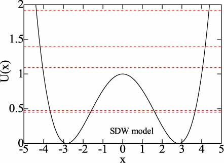
Figure 1: (Color online) The symmetric DW potential (solid curve) with $x_{s}=2\sqrt{2}$ and $\Delta=1.0$ in Eq. (7), dashed curves expressing eigenvalues of $E_{\nu}$ ($\nu=0-4$).

II.2 Spectral method

Various approximate analytical and numerical methods have been proposed to solve the Schrödinger equation given by Eq. (1) Tannor07 . Assuming $\Psi(x,t)=\Psi(x)\>e^{-iEt/\hbar}$, we first solve the steady-state Schrödinger equation, $H\Psi(x)=E\Psi(x)$, with the eigenvalue $E$. The stationary wavefunction $\Psi(x)$ is expanded in terms of $\phi_{n}(x)$

$$\Psi(x) = \sum_{n=0}^{N_{m}}c_{n}\phi_{n}(x),$$ (13)

leading to the secular equation

$$Ec_{n} = \sum_{k=0}^{N_{m}}H_{nk}c_{k},$$ (14)

with

$$H_{nk} = E_{0n}\>\delta_{n,k}+\int_{-\infty}^{\infty}\phi_{n}(x)^{*}\>V(x)\phi_{k}(x)\;dx,$$ (15)

where $N_{m}$ is the maximum quantum number.

For the time-dependent state, we adopt SM in which the eigenfunction $\Psi(x,t)$ is expanded in terms of $\phi_{n}(x)$ with finite $N_{m}$

$$\Psi(x,t) = \sum_{n=0}^{N_{m}}c_{n}(t)\phi_{n}(x).$$ (16)

Time-dependent expansion coefficients $\{c_{n}(t)\}$ obey equations of motion given by

$$i\hbar\>\frac{\partial c_{n}(t)}{\partial t} = \sum_{k=0}^{N_{m}}H_{nk}\>c_{k}(t)\hskip 28.45274pt\mbox{($n=0$ to $N_{m}$)}.$$ (17)

Equation (17) expresses the ($N_{m}+1$) first-order differential equations, which may be solved for given initial conditions of $\{c_{n}(0)\}$. Initial values of expansion coefficients $\{c_{n}(0)\}$ are determined by

$$c_{n}(0) = \int_{-\infty}^{\infty}\phi_{n}(x)^{*}\>\Psi_{G}(x,0)\>dx\hskip 28.45274pt\mbox{($n=0$ to $N_{m}$)},$$ (18)

for a given Gaussian wavepacket $\Psi_{G}(x,0)$ [Eq. (5)]

$$\Psi_{G}(x,0)=\frac{1}{(2\pi\mu_{0})^{1/4}}\>\exp\left[-\frac{(1-i\alpha_{0})}{4\mu_{0}}(x-x_{0})^{2}+i\>\frac{p_{0}(x-x_{0})}{\hbar}\right],$$ (19)

where $x_{0}$ and $p_{0}$ are initial position and momentum, respectively, and $\mu_{0}$ and $\alpha_{0}$ are assumed initial parameters at $t=0.0$. Once solutions of $\{c_{n}(t)\}$ in Eq. (17) are obtained, the wavefunction $\Psi(x,t)$ may be constructed by Eq. (16).

Matrix elements $H_{nk}$ in Eq. (15) may be analytically evaluated, and various time-dependent averages such as $\langle x\rangle$ and $\langle p\rangle$ are expressed in terms of $\{c_{n}(t)\}$ (see the Appendix). We expect that SM with $N_{m}=30$ adopted in our numerical calculations is fairly accurate Hasegawa12b ; Hasegawa13b . Some results of SM have been cross-checked, by solving the Schrödinger equation with the use the MATHEMATICA resolver for the partial differential equation.

II.3 Time-dependent variational approximation

Equations of motion in Eq. (2) are expressed by

$$\frac{d\langle x\rangle}{dt} = \frac{\langle p\rangle}{m},$$ (20)

$$\frac{d\langle p\rangle}{dt} = -U^{\prime}(\langle x\rangle)-\sum_{k=2}^{\infty}\frac{U^{(k+1)}(\langle x\rangle)}{k!}\langle\delta x^{k}\rangle,$$ (21)

$$\frac{d\langle\delta x^{2}\rangle}{dt} = \frac{1}{m}\langle\delta x\delta p+\delta p\delta x\rangle,$$ (22)

$$\frac{d\langle\delta x\delta p+\delta p\delta x\rangle}{dt} = -2\sum_{k=1}^{\infty}\frac{U^{(k+1)}(\langle x\rangle)}{k!}\langle\delta x^{k+1}\rangle+\frac{2}{m}\langle\delta p^{2}\rangle,$$ (23)

$$\frac{d\langle\delta p^{2}\rangle}{dt} = -\sum_{k=1}^{\infty}\frac{U^{(k+1)}(\langle x\rangle)}{k!}\langle\delta x^{k}\delta p+\delta p\delta x^{k}\rangle.$$ (24)

Equations (20)-(24) include higher-order fluctuations which are not closed in general. It is possible to construct various approximations depending on how many terms are taken into account in Eqs. (20)-(24). If we neglect the second term of Eq. (21), Eqs. (20) and (21) form classical equations of motion. When we neglect the second term in Eq. (21) and truncate Eqs. (23) and (24) at $k=1$, Eqs. (20)-(24) reduce to equations of motion in Heller’s GWM. Equations of motion including up to fourth-order corrections were obtained in Ref. Sundaram95 .

To close a hierarchal chain of equations of motion, TDVA assumes that a wavepacket is expressed by the normalized squeezed coherent state given by Eq. (5), implying relations Cooper86 ; Pattanayak94 ; Pattanayak94b ; Sundaram95

$$\langle\delta x^{2\ell}\rangle = \frac{(2\ell)!}{\ell!\>2^{\ell}}\>\mu^{\ell},\;\;\;\;\langle\delta x^{2\ell+1}\rangle=0,\hskip 14.22636pt\mbox{$(\ell=1,2,\cdot\cdot)$}$$ (25)

$$\langle\delta p^{2}\rangle = \frac{\hbar^{2}+\alpha^{2}}{4\mu},$$ (26)

$$\langle\delta x\delta p+\delta p\delta x\rangle = \alpha,$$ (27)

where $\mu$ and $\alpha$ are time-dependent parameters. Note that Eqs. (25)-(27) yield the uncertainty product expressed by

$$\langle\delta x^{2}\rangle\langle\delta p^{2}\rangle = \frac{\hbar^{2}+\langle\delta x\delta p+\delta p\delta x\rangle^{2}}{4}.$$ (28)

These lead to equations of motion given by

$$\frac{d\langle x\rangle}{dt} = \frac{\langle p\rangle}{m},$$ (29)

$$\frac{d\langle p\rangle}{dt} = -U^{\prime}(\langle x\rangle)-\sum_{\ell=1}^{\infty}\frac{U^{(2\ell+1)}(\langle x\rangle)}{\ell!\;2^{\ell}}\>\mu^{\ell},$$ (30)

$$\frac{d\mu}{dt} = \frac{\alpha}{m},$$ (31)

$$\frac{d\alpha}{dt} = \frac{\hbar^{2}+\alpha^{2}}{2m\mu}-\sum_{\ell=1}^{\infty}\frac{U^{(2\ell)}(\langle x\rangle)}{(\ell-1)!\;2^{\ell-2}}\>\mu^{\ell}.$$ (32)

Alternatively, Eqs. (29)-(32) may be rewritten as

$$\frac{d\langle x\rangle}{dt} = \frac{\langle p\rangle}{m},$$ (33)

$$\frac{d\langle p\rangle}{dt} = -U^{\prime}(\langle x\rangle)-\sum_{\ell=1}^{\infty}\frac{U^{(2\ell+1)}(\langle x\rangle)\langle\delta x^{2}\rangle^{\ell}}{\ell!\;2^{\ell}},$$ (34)

$$\frac{d\langle\delta x^{2}\rangle}{dt} = \frac{1}{m}\langle\delta x\delta p+\delta p\delta x\rangle,$$ (35)

$$\frac{d\langle\delta x\delta p+\delta p\delta x\rangle}{dt} = \frac{\hbar^{2}+\langle\delta x\delta p+\delta p\delta x\rangle^{2}}{2m\langle\delta x^{2}\rangle}-\sum_{\ell=1}^{\infty}\frac{U^{(2\ell)}(\langle x\rangle)\langle\delta x^{2}\rangle^{\ell}}{(\ell-1)!\>2^{\ell-2}},$$ (36)

which show a closure of equations of motion within $\langle x\rangle$, $\langle p\rangle$, $\langle\delta x^{2}\rangle$ and $\langle\delta x\delta p+\delta p\delta x\rangle$.

III Model calculations

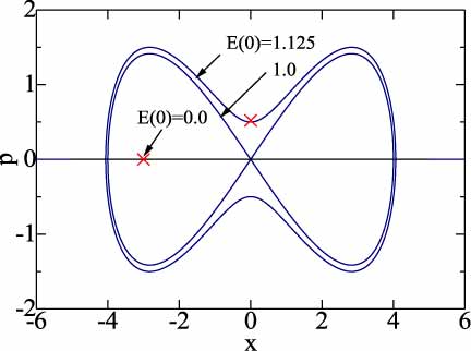
Figure 2: (Color online) The classical $x$-$p$ phase space of the SDW model for various initial energies of $E(0)$, marks $\times$ denoting positions of initial states adopted in model calculations.

We apply our calculation method to the SDW potential given by Eq. (7). We have calculated energy matrix elements of $H_{kn}$, by using Eq. (A5) with $m=\omega=\hbar=1.0$ and $N_{m}=30$. Obtained eigenvalues are $E_{\nu}=$ 0.450203, 0.474126, 1.09262, 1.39334 and 1.91286 for $\nu=0$ to 4, respectively, which are plotted by dashed curves in Fig. 1. The ground state ($E_{0}$) and first excited state ($E_{1}$), which are quasi-degenerate, are below the potential barrier of $\Delta=1.0$. The energy gap between ground and first excited states is $\Delta E=E_{1}-E_{0}=0.023923$. Low-lying eigenvalues calculated with $N_{m}=30$ are in good agreement with those obtained with $N_{m}=20$ Hasegawa12b .

Figure 2 shows the classical $x$-$p$ phase space for initial energies of $E(0)=0.0$, 1.0 and 1.125. Marks $\times$ in Fig. 2 show two initial states in the $x$-$p$ phase space adopted in our calculations. Calculated results for the two initial states of $(x_{0},p_{0})=(-2\sqrt{2},0.0)$ and $(x_{0},p_{0})=(0.0,0.5)$ will be separately reported in the following.

III.0.1 Case of the initial state of $(x_{0},p_{0})=(-2\sqrt{2},0.0)$

We have adopted the Gaussian wavepacket $\Psi_{G}(x,0)$ locating at the stable point of the left well with $(x_{0},p_{0})=(-2\sqrt{2},0.0)$, and $\mu_{0}=0.1$ and $\alpha_{0}=0.0$ at $t=0.0$, which yields the minimum uncertainty product of $\langle\delta x^{2}\rangle\langle\delta p^{2}\rangle=1/4$. Initial coefficients $\{c_{n}(0)\}$ calculated by Eq. (18) are real with appreciable magnitudes for $3\lesssim n\lesssim 10$. A norm of the initial Gaussian wavepacket is $\sum_{n}c_{n}(0)^{*}c_{n}(0)=0.999999$ [Eq. (A7)]. After solving ($N_{m}+1$) first-order differential equations for $\{c_{n}(t)\}$ given by Eq. (17) for initial values of $\{c_{n}(0)\}$, we obtain the time-dependent eigenfunction $\Psi(x,t)$ expressed in terms of $\{c_{n}(t)\}$ in Eq. (16).

Figure 3 shows the 3D plot of $|\Psi(x,t)|^{2}$ calculated by SM. We note that the Gaussian wavepacket in SM quickly spreads as the time develops. In order to scrutinize the behavior of $|\Psi(x,t)|^{2}$ at small $t$, its time dependence at $0\leq t\leq 25$ is plotted by bold solid curves in Fig. 4, where solid curves denote results of TDVA. The Gaussian wavepacket becomes widespread even at $t=5.0$ in SM, and its trend becomes more significant with increasing $t$. Figure 4 clearly shows that $|\Psi(x,t)|^{2}$ in SM is quite different from that in TDVA and that $\Psi(x,t)$ cannot be expressed by a single Gaussian except at $t=0.0$.

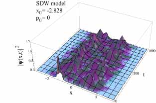
Figure 3: (Color online) 3D plot of $|\Psi(x,t)|^{2}$ as functions of $x$ and $t$ calculated by SM for the SDW model ($x_{0}=-2\sqrt{2},p_{0}=0.0$).

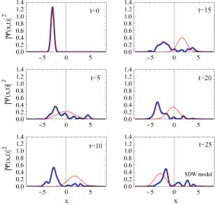
Figure 4: (Color online) The $x$ dependence of $|\Psi(x,t)|^{2}$ at various $t$ of the SDW model calculated by SM (bold solid curves) and TDVA (solid curve) ($x_{0}=-2\sqrt{2},p_{0}=0.0$).

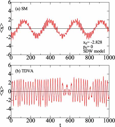
Figure 5: (Color online) The time dependence of $\langle x\rangle$ of the SDW model calculated by (a) SM and (b) TDVA ($x_{0}=-2\sqrt{2},p_{0}=0.0$).

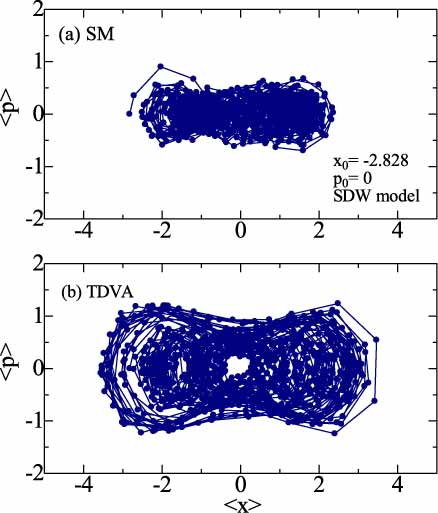
Figure 6: (Color online) The $\langle x\rangle$ vs. $\langle p\rangle$ plot of the SDW model calculated by (a) SM and (b) TDVA, time step being $\Delta t=1.0$ for $0\leq t<1000$ ($x_{0}=-2\sqrt{2},p_{0}=0.0$).

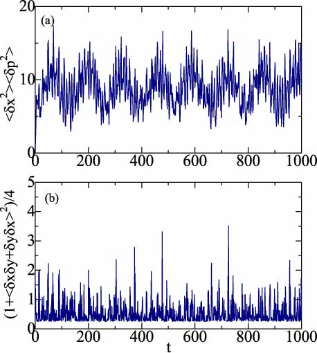
Figure 7: (Color online) Time dependences of (a) the uncertainty product of $\langle\delta x^{2}\rangle\langle\delta p^{2}\rangle$ and (b) $(1+\langle\delta x\delta p+\delta x\delta p\rangle^{2})/4$ of the SDW model calculated by SM ($x_{0}=-2\sqrt{2},p_{0}=0.0$). Note that $\langle\delta x^{2}\rangle\langle\delta p^{2}\rangle$ equals to $(1+\langle\delta x\delta p+\delta x\delta p\rangle^{2})/4$ in TDVA [Eq. (28)], which is not realized in (a) and (b).

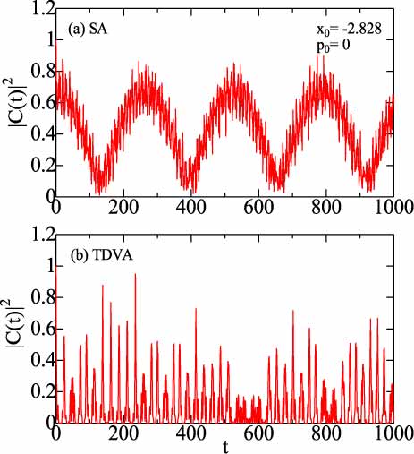
Figure 8: (Color online) Time dependences of the auto-correlation function $|C(t)|^{2}$ of the SDW model calculated by (a) SM and (b) TDVA ($x_{0}=-2\sqrt{2},p_{0}=0.0$).

The difference between SM and TDVA is more clearly seen in the time-dependent expectation value of $\langle x\rangle$. Figure 5(a) shows $\langle x\rangle$ of SM expressing a tunneling of a particle with the period of about 260, which is consistent with the period estimated from the energy gap by $T=2\pi/\Delta E=262$. On the contrary, $\langle x\rangle$ of TDVA in Fig. 5(b) shows more rapid oscillation with a period of about $25-30$.

Figures 6(a) and 6(b) show $\langle x\rangle$ vs. $\langle p\rangle$ plots calculated by SM and TDVA, respectively. The $\langle x\rangle$ vs. $\langle p\rangle$ plot of SM in Fig. 6(a) is quite different from that of TDVA in Fig. 6(b).

Figure 7(a) shows the uncertain product of $\langle\delta x^{2}\rangle\langle\delta p^{2}\rangle$ calculated by SM, which expresses a measure of quantum fluctuation. It starts from the minimum uncertainty of $1/4$ at $t=0$, and with increasing $t$ it grows and oscillates between about 5 and 17 with the period of about 130. For a comparison, we plot $(1+\langle\delta x\delta p+\delta x\delta p\rangle^{2})/4$ in Fig. 7(b). TDVA assumes the equality of $\langle\delta x^{2}\rangle\langle\delta p^{2}\rangle=(1+\langle\delta x\delta p+\delta x\delta p\rangle^{2})/4$ as given by Eq. (28). Figures 7(a) and 7(b), however, imply that this equality is not satisfied in SM.

Figures 8(a) and 8(b) show the auto-correlation functions $|C(t)|^{2}$ calculated by SM and TDVA, respectively, with Eq. (A7) in the Appendix. $|C(t)|^{2}$ of SM, which is unity at $t=0.0$, oscillates between about 0.1 and 0.7 with a period of about 260. The result of SM in Fig. 8(a) is again quite different from that of TDVA in Fig. 8(b).

III.0.2 Case of the initial state of $(x_{0},p_{0})=(0.0,0.5)$

Next we adopt a Gaussian wavepacket with a different initial state of $(x_{0},p_{0})=(0.0,0.5)$ but with the same $\mu_{0}=0.1$ and $\alpha_{0}=0.0$ at $t=0.0$. Initial coefficients $\{c_{n}(0)\}$ calculated by Eq. (18) are complex with appreciable magnitudes for $0\lesssim n\lesssim 15$. The initial state of $(x_{0},p_{0})=(0.0,0.5)$ locates near a top of the potential barrier (see Fig. 2). Note that in the classical calculation, the $x$ vs. $p$ plot forms a cocoon shape extending from $x=-4.06021$ to $x=4.06021$ and from $p=-1.5$ to 1.5, as shown in Fig. 2. Then at $t>0$, a particle starting from $(x_{0},p_{0})=(0.0,0.5)$ rolls down the potential up to $x=4.06021$ and then approaches $x=-4.06021$ after passing through $x=0$ in the classical calculation. However, this classical behavior is quite different from quantum results calculated by SM and TDVA. The 3D plot of $|\Psi(x,t)|^{2}$ of SM shown in Fig. 9 has appreciable magnitudes at $-5\lesssim x\lesssim 5$ for $0<t<1000$. Bold solid curves and solid curves in Fig. 10 show $|\Psi(x,t)|^{2}$ calculated by SM and TDVA, respectively. $|\Psi(x,t)|^{2}$ of SM, which is distorted and spreads at $t>0$, is different from the relevant result of TDVA. An expectation value of $\langle x\rangle$ of SM in Fig. 11(a) does not so much depart from the initial point of $x=0.0$ in contrast to that of TDVA shown in Fig. 11(b).

Figures 12(a) and 12(b) show $\langle x\rangle$ vs. $\langle p\rangle$ plots calculated by SM and TDVA, respectively. The result of SM in Fig. 12(a) exhibits a random-like motion, which is different from a quasi-periodic motion of TDVA in Fig. 12(b).

Figures 13(a) and 13(b) show $\langle\delta x^{2}\rangle\langle\delta p^{2}\rangle$ and $(1+\langle\delta x\delta p+\delta x\delta p\rangle^{2})/4$, respectively, calculated by SM. We note that $\langle\delta x^{2}\rangle\langle\delta p^{2}\rangle\neq(1+\langle\delta x\delta p+\delta x\delta p\rangle^{2})/4$ in SM, which is in contrast with Eq. (28) in TDVA.

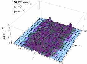
Figure 9: (Color online) 3D plot of $|\Psi(x,t)|^{2}$ as functions of $x$ and $t$ calculated by SM for the SDW model ($x_{0}=0.0,p_{0}=0.5$).

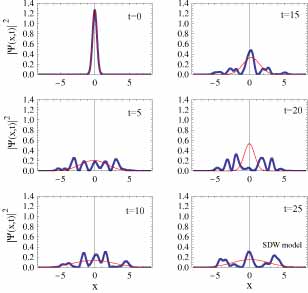
Figure 10: (Color online) The $x$ dependence of $|\Psi(x,t)|^{2}$ at various $t$ of the SDW model calculated by SM (bold solid curves) and TDVA (solid curves) ($x_{0}=0.0,p_{0}=0.5$).

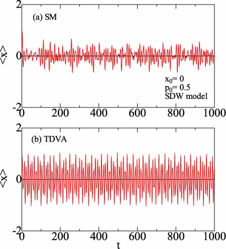
Figure 11: (Color online) Time dependences of $\langle x\rangle$ of the SDW model calculated by (a) SM and (b) TDVA ($x_{0}=0.0,p_{0}=0.5$).

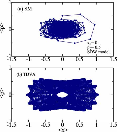
Figure 12: (Color online) The $\langle x\rangle$ vs. $\langle p\rangle$ plot of the SDW model calculated by (a) SM and (b) TDVA, time step being $\Delta t=1.0$ for $0\leq t<1000$ ($x_{0}=0.0,p_{0}=0.5$).

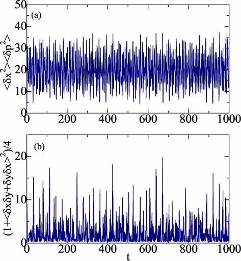
Figure 13: (Color online) Time dependences of (a) the uncertainty product of $\langle\delta x^{2}\rangle\langle\delta p^{2}\rangle$ and (b) $(1+\langle\delta x\delta p+\delta x\delta p\rangle^{2})/4$ of the SDW model calculated by SM ($x_{0}=0.0,p_{0}=0.5$). Note that $\langle\delta x^{2}\rangle\langle\delta p^{2}\rangle$ equals to $(1+\langle\delta x\delta p+\delta x\delta p\rangle^{2})/4$ in TDVA [Eq. (28)], which is not held in SM.

IV Discussion

IV.1 An effective Hamiltonian in TDVA

Refs. Cooper86 ; Pattanayak94 ; Pattanayak94b showed that by using a change of variables given by

$$\rho^{2} = \langle\delta x^{2}\rangle,$$ (37)

$$\pi = \frac{1}{2\rho}\langle\delta x\delta p+\delta p\delta x\rangle,$$ (38)

Eqs. (29)-(32) are transformed to

$$\frac{d\langle x\rangle}{dt} = \frac{\langle p\rangle}{m},$$ (39)

$$\frac{d\langle p\rangle}{dt} = -U^{\prime}(\langle x\rangle)-\sum_{\ell=1}^{\infty}\frac{U^{(2\ell+1)}(\langle x\rangle)}{\ell!\;2^{\ell}}\rho^{2\ell},$$ (40)

$$\frac{d\rho}{dt} = \frac{\pi}{m},$$ (41)

$$\frac{d\pi}{dt} = \frac{\hbar^{2}}{4m\rho^{3}}-\sum_{\ell=1}^{\infty}\frac{U^{(2\ell)}(\langle x\rangle)}{(\ell-1)!\;2^{\ell-1}}\rho^{2\ell-1}.$$ (42)

It was shown that fluctuation variables $\rho$ and $\pi$ are conjugate and that the effective Hamiltonian may be expressed in the extended phase space spanned by $\langle x\rangle$, $\langle p\rangle$, $\rho$ and $\pi$ as given by Cooper86 ; Pattanayak94 ; Pattanayak94b

$$H_{eff} = \frac{\langle p\rangle^{2}}{2m}+\frac{\pi^{2}}{2m}+\frac{\hbar^{2}}{8m\rho^{2}}+U(\langle x\rangle)+\sum_{\ell=1}^{\infty}\frac{U^{(2\ell)}(\langle x\rangle)}{\ell!\>2^{\ell}}\rho^{2\ell}.$$ (43)

We should note that the effective Hamiltonian given by Eq. (43) relies on the identities given by Eqs. (25)-(27) which are based on the assumed squeezed Gaussian wavepacket given by Eq. (5). If these identities are not held as our SM calculation suggests, the effective Hamiltonian given by Eq. (43) is not valid in DW systems.

IV.2 Anharmonic Oscillator

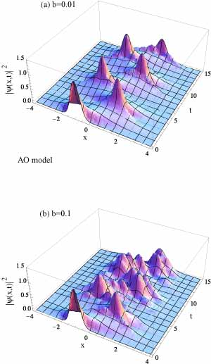
Figure 14: (Color online) 3D plot of $|\Psi(x,t)|^{2}$ as functions of $x$ and $t$ of the AO model with (a) $b=0.01$ and (b) $b=0.1$ calculated by SM ($x_{0}=-1.0,p_{0}=0.0$).

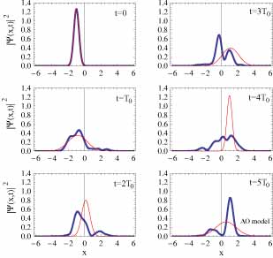
Figure 15: (Color online) The $x$ dependence of $|\Psi(x,t)|^{2}$ at $t=kT_{0}$ ($k=0,1,2\cdots$) of the AO model with $b=0.1$ calculated by SM (bold solid curves) and TDVA (solid curve) ($x_{0}=-1.0,p_{0}=0.0$), where $T_{0}=6.283$ $(=2\pi/\omega)$ is a period for a HO system ($b=0$).

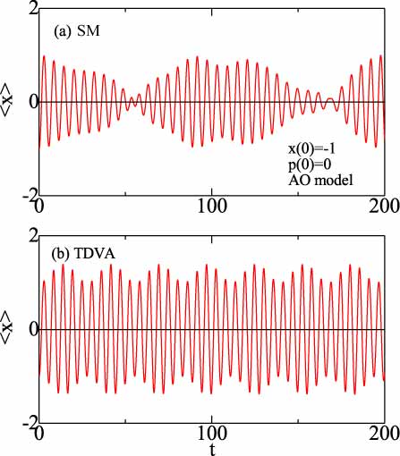
Figure 16: (Color online) Time dependences of $\langle x\rangle$ in the AO model with $b=0.1$ calculated by (a) SM and (b) TDVA ($x_{0}=-1.0,p_{0}=0.0$).

We have studied Gaussian wavepacket dynamics of quantum DW systems in the preceding section. It is worthwhile to examine also an AO model given by

$$U(x) = \frac{x^{2}}{2}+\frac{bx^{4}}{4}=U_{0}(x)+\frac{bx^{4}}{4},$$ (44)

where $b$ expresses a degree of anharmonicity. We have repeated calculations, by using SM and TDVA with necessary modifications.

Figure 14(a) shows the 3D plot of $|\Psi(x,t)|^{2}$ for $b=0.01$ with an assumed Gaussian state for $(x_{0},p_{0})=(-1.0,0.0)$, and $\mu_{0}=0.1$ and $\alpha_{0}=0.0$ at $t=0.0$. In the case of a HO potential ($b=0.0$), $|\Psi(x,t)|^{2}$ is periodic with a period of $T_{0}=2\pi/\omega=6.283$. It is shown in 14(a) that $|\Psi(x,t)|^{2}$ for a small $b=0.01$ is nearly periodic as that for $b=0.0$ at $t<10$. For a larger $b=0.1$, however, this periodicity is destroyed and the wavepacket spreads in the non-Gaussian form as Fig. 14(b) shows. This is more clearly realized in Fig. 15 where $|\Psi(x,t)|^{2}$ calculated by SM (bold solid curves) are quite different from their counterparts obtained by TDVA (solid curve). Our result of SM in Fig. 15 is consistent with that in Ref. Herrera12 which studied effects of anharmonicity and interactions in DW systems.

Figures 16(a) and 16(b) show time dependences of $\langle x\rangle$ calculated by SM and TDVA, respectively. $\langle x\rangle$ oscillates with a period of about $5.6$ in both results. However, a period of its envelope variation in SM ($\sim 110$) is larger than that in TDVA ($\sim 30$): the former corresponds to the revival time after which a wavepacket periodically returns to the initial shape.

V Conclusion

By using SM and TDVA, we have calculated time dependences of wavefunctions, averages of position and momentum, auto-correlation function, and uncertainty product in quantum SDW systems. The validity of TDVA has been examined by comparisons between results of SM and TDVA. We have obtained following results:

(1) An initial Gaussian wavepacket in DW systems of SM spreads and deforms at $t>0$ where a wavepacket cannot be expressed by a single Gaussian in contrast to TDVA,

(2) Time dependences of expectation values of $\langle x\rangle$ and $\langle p\rangle$, and the auto-correlation function in SM are quite different from their counterparts in TDVA, and

(3) The identity relation for uncertainty product assumed in TDVA [Eq. (28)] is not satisfied in SM.

The item (1) holds also in asymmetric DW systems Hasegawa13b . The item (2) implies that the tunneling phenomenon characteristic in DW systems cannot be well accounted for in TDVA (Fig. 5) Hasegawa13b . The item (3) suggests that the effective Hamiltonian in the extended phase space given by Eq. (43) does not hold in DW systems because it is derived with the squeezed Gaussian wavepacket with assumptions given by Eqs. (25)-(27) in TDVA. GWM is best applied to dynamics in HO and AO with a small anharmonicity, for which it provides us with an efficient and physically-transparent calculation method. Our calculations, however, point out that GWM is not a good approximation for DW systems. For a better description of quantum DW systems, it might be necessary to adopt extended GWMs with superimposed multiple Gaussian wavepackets (see Ref. Zoppe05 , related references therein), which are much sophisticated and complicated than the original Heller’s GWM Heller75 .

*

Appendix A Matrix elements and various expectation values

Matrix elements $H_{nk}$ in Eq. (15) are given as follows: We rewrite the potential $U(x)$ as

$$U(x) = \frac{A_{4}x^{4}}{4}+\frac{A_{3}x^{3}}{3}+\frac{A_{2}x^{2}}{2}+A_{1}x+A_{0},$$ (A1)

with

$$A_{4} = \frac{m\omega^{2}}{2x_{s}^{2}},\;\;A_{3}=0,\;\;A_{2}=-\frac{m\omega^{2}}{2},\;\;A_{1}=0,\;\;A_{0}=\frac{m\omega^{2}x_{s}^{2}}{8}.$$ (A2)

By using relations given by

$$q = \sqrt{\frac{g}{2}}(a^{\dagger}+a),\;\;\;p=i\frac{\hbar}{\sqrt{2g}}(a^{\dagger}-a),\hskip 28.45274pt\mbox{$\left(g=\frac{\hbar}{m\omega}\right)$}$$ (A3)

$$a^{\dagger}\>\phi_{n} = \sqrt{n+1}\>\phi_{n+1},\;\;a\>\phi_{n}=\sqrt{n}\>\phi_{n-1},$$ (A4)

we obtain the symmetric matrix elements $H_{nk}$ for $n\geq k$ given by

$$H_{nk} = \left[\left(n+1/2\right)\hbar\omega+\frac{3A_{4}g^{2}}{16}(2n^{2}+2n+1)+\frac{A_{2}^{\prime}\>g}{2}(n+1/2)+A_{0}\right]\>\delta_{n,k}$$ (A5)

$$+ \left[A_{3}\left(\frac{g}{2}\right)^{3/2}n\sqrt{n}+A_{1}\left(\frac{g}{2}\right)^{1/2}\sqrt{n}\right]\delta_{n-1,k}$$

$$+ \left[\frac{A_{4}g^{2}}{8}(n-1)\sqrt{n(n-1)}+\frac{A_{2}^{\prime}\>g}{4}\sqrt{n(n-1)}\right]\>\delta_{n-2,k}$$

$$+ \frac{A_{3}}{3}\left(\frac{g}{2}\right)^{3/2}\sqrt{n(n-1)(n-2)}\>\delta_{n-3,k}$$

$$+ \frac{A_{4}g^{2}}{16}\sqrt{n(n-1)(n-2)(n-3)}\>\delta_{n-4,k},$$

where $A_{2}^{\prime}=A_{2}-m\omega^{2}$.

Various time-dependent quantities may be expressed in terms of $\{c_{n}(t)\}$ as follows: After some manipulations with the use of the relations given by Eqs.(A3) and (A4), the auto-correlation function is given by

$$C(t) = \int_{-\infty}^{\infty}\Psi(x,t)^{*}\Psi(x,0)\>dx,$$ (A6)

$$= \sum_{n=0}^{N_{m}}c_{n}(t)^{*}\>c_{n}(0),$$ (A7)

and expectation values such as $x(t)$ and $p(t)$ are expressed by

$$\langle x(t)\rangle = \sqrt{\frac{g}{2}}\sum_{n}\left[\sqrt{n+1}\>c_{n+1}^{*}(t)c_{n}(t)+\sqrt{n}\>c_{n-1}^{*}(t)c_{n}(t)\right],$$ (A8)

$$\langle p(t)\rangle = i\sqrt{\frac{\hbar^{2}}{2g}}\sum_{n}\left[\sqrt{n+1}\>c_{n+1}^{*}(t)c_{n}(t)-\sqrt{n}\>c_{n-1}^{*}(t)c_{n}(t)\right],$$ (A9)

$$\langle x(t)^{2}\rangle = \left(\frac{g}{2}\right)\sum_{n}[\sqrt{(n+1)(n+2)}\>c_{n+2}^{*}(t)c_{n}(t)+(2n+1)\>c_{n}^{*}(t)c_{n}(t)$$ (A10)

$$+ \sqrt{n(n-1)}\>c_{n-2}^{*}(t)c_{n}(t)],$$

$$\langle p(t)^{2}\rangle = -\left(\frac{\hbar^{2}}{2g}\right)\sum_{n}[\sqrt{(n+1)(n+2)}\>c_{n+2}^{*}(t)c_{n}(t)-(2n+1)\>c_{n}^{*}(t)c_{n}(t)$$ (A11)

$$+ \sqrt{n(n-1)}\>c_{n-2}^{*}(t)c_{n}(t)],$$

$$\langle x(t)p(x)+p(t)x(t)\rangle = i\>\hbar\sum_{n}[\sqrt{(n+1)(n+2)}\>c_{n+2}^{*}(t)c_{n}(t)$$ (A12)

$$- \sqrt{n(n-1)}\>c_{n-2}^{*}(t)c_{n}(t)].$$

References

- (1) D. J. Tannor, Introduction to quantum mechanics: A time-dependent perspective (Univ. Sci. Books, Sausalito, California, 2007).
- (2) R.W. Robinett, Phys. Rep. 392 (2004) 1.
- (3) E. J. Heller, J. Chem. Phys. 62 (1975) 1544.
- (4) E. J. Heller, J. Chem. Phys. 75 (1981) 2923.
- (5) D. Huber and E. J. Heller, J. Chem. Phys. 87 (1987) 5302.
- (6) F. Cooper, S.-Y. Pi, and P. N. Stancioff, Phys. Rev. D 34 (1986) 3831.
- (7) Y. Tsue and Y. Fujiwara, Prog. Theo. Phys. 86 (1991) 443.
- (8) A. K. Pattanayak and W. C. Schieve, Phys. Rev. Lett. 72 (1994) 2855.
- (9) A. K. Pattanayak and W. C. Schieve, Phys. Rev. E 50 (1994) 3601.
- (10) B. Sundaram and P. W. Milonni, Phys. Rev. E 51 (1995) 1971.
- (11) M. Thorwart, M. Grifoni, and P. Hänggi, Annals Phys. 293 (2001) 14.
- (12) W. A. Lin, L. E. Ballentine, Phys. Rev. Lett. 65 (1990) 2927; Phys. Rev. A 45 (1992) 3637.
- (13) R. Utermann, T. Dittrich, and P. Hänggi, Phys. Rev. E 49 (1994) 273.
- (14) K. Husimi, Proc. Phys. Math. Soc. Jpn. 22 (1940) 264.
- (15) A. Igarashi, and H. Yamada, Physica D 221 (2006) 146.
- (16) Y. Ashkenazy, L. P. Horwitz, J. Levitan, M. Lewkowicz, and Y. Rothschild, Phys. Rev. Lett. 75 (1995) 1070.
- (17) A. K. Pattanayak and W. C. Schieve, Phys. Rev. A 54 (1996) 947.
- (18) T. C. Blum and Hans-Thomas Elze, Phys. Rev. E 53 (1996) 3123.
- (19) O. F. de Alcantara Bonfim, J. Florencio and F. C. Sa Barreto, Phys. Rev. E 58 (1998) 6851.
- (20) B. C. Bag and D. S. Ray, Phys. Rev. E 61 (2000) 3223.
- (21) A. Roy and J. K. Bhattacharjee, Phys. Letters A 288 (2001) 1.
- (22) S. Habib, arXiv:0406011.
- (23) H. Hasegawa, Phys. Rev. E 86 (2012) 061104.
- (24) H. Hasegawa, Physica A 392 (2013) 6232.
- (25) M. Herrera, T. M. Antonsen, E. Ott, and S. Fishman, arXiv:1212.2850.
- (26) J. O. Zoppe, M. L. Parkinson, M. Messina, Chem. Phys. Lett. 407 (2005) 308.