Symmetries and optical transitions of hexagonal quantum dots in GaAs/AlGaAs nanowires

Abstract

We investigate the properties of electronic states and optical transitions in hexagonal GaAs quantum dots within Al_0.3Ga_0.7As nanowires. Such dots are particularly interesting due to their high degree of symmetry. A streamlined postsymmetrization technique based on class operators (PTCO) is developed which enables one to benefit in one run from the insight brought by the Maximal symmetrization and reduction of fields (MSRF) approach reported by Dalessi et al.Dalessi and Dupertuis (2010), after having solved the Schrödinger equation. Definite advantages of the PTCO are that it does not require having to modify any existing code for the calculation of the electronic structure, and that it allows to numerically test for elevated symmetries. We show in the frame of a 4-band $k\cdot{p}$ model that despite the fact that the D${}_{\textrm{6h}}$ symmetry of the nanostructure is broken at the microscopic level by the underlying Zinc Blende crystal structure, the effect is quite small. Most of the particularities of the electronic states and their optical emission can be understood by symmetry elevation to D${}_{\textrm{6h}}$ and the presence of approximate azimuthal and radial quantum numbers.

I introduction

Semiconductor nanowires have emerged as promising building blocks for realization of various nanoscale optoelectronic devices Lauhon et al. (2004). The nanowire technologies enable heterostructures with a high level of flexibility in terms of geometry and material composition Lauhon et al. (2004). In particular, growth of site controlled quantum dots (QDs) within nanowires show significant advantages compared to more conventional self-assembled QDs (Stranski-Krastanov)Tribu et al. (2008); Borgström et al. (2005), and bright single photon emitters have been demonstrated in a range of materials using nanowire QDsKats et al. (2012); Tribu et al. (2008); Borgström et al. (2005); Choi et al. (2012); Dorenbos et al. (2010).

QDs may be used to facilitate quantum information and cryptography technologies, e.g. by emission of entangled photon pairs. In this respect nanowire QDs are especially suitable as they are highly symmetric, with a hexagonal cross section. High symmetry is a requisite for entanglement, needed in order to limit the fine structure splitting of the excitonic states which is a consequence of symmetry breaking. QDs within nanowires grown in the high symmetry direction [111] are therefore suggested as ideal sources for emission of entangled photon pairs Singh and Bester (2009). Cascaded emission spectra, possibly enabling such pairs have also been measured experimentally Dorenbos et al. (2010). Generation of entangled photons is also possible in self-assembled QDs, especially InGaAs/GaAs QDs grown on [111] substrates are proposed ideal for such generation, due to the threefold rotation symmetry of this surfaceSchliwa et al. (2009). QDs may also enable quantum computation by using the electron spin as a quantum bit Imamoglu et al. (1999), QDs grown in inverted pyramids on [111] GaAs substrates Oberli et al. (2009) are also promising in this respect.

With increasing control of heterostructure shape and material composition, comes the possibility to grow structures according to optimized design. Theoretical models e.g. providing insight into the nature of electronic states are essential in such optimization. In this work we calculate the electronic states and optical transitions in hexagonal GaAs/AlGaAs nanowire QDs, and analyze the results taking advantage of their high symmetry. A detailed procedure for full-depth symmetry analysis and reduction of computational domain has been presented previously by Dalessi et al.Dalessi and Dupertuis (2010). Here we will pursue this effort by developing a new procedure alleviating recoding: a postsymmetrization technique using class operators (PTCO). The PTCO is very general and applies independently of the method employed for the calculation of the electronic structure ($k\cdot{p}$, tight-binding e.t.c). It also provides a systematic and flexible procedure to test possible elevated symmetries.

In Sec. II relevant theoretical studies of similar semiconductor heterostructures are considered, and we present the general features of the $k\cdot{p}$ model used in this paper. The explicit QD under consideration is described in Sec. III, and the symmetries of our model structure are identified, providing the premises to optimally choose the basis of our $k\cdot{p}$ Hamiltonian. Having fully specified the numerical model, we describe the pertaining symmetry implications on the QD eigenstates in Sec. IV. The PTCO is then presented in Sec. V. Secs. VI and VII contain the numerical calculations, analyzed using the PTCO. We show in Sec. VI that the analysis gives rise to a deeper understanding of the electronic states, in particular of the level sequences. In Sec. VII we investigate the fine structure of the spectrum of squared momentum matrix elements. We prove that symmetry elevation to D${}_{\textrm{6h}}$ and the existence of azimuthal and radial quantum numbers are necessary ingredients to explain many missing/weak transitions.

II Quantum dot description and $k\cdot{p}$ model

Despite large activity within the experimental realization of nanowire QDs, there has until now been much less attention towards numerical calculations of the electronic states. Niquet et al.Niquet and Mojica (2008) did perform calculations of strained InAs/InP nanowire QDs, using a tight binding model. The optical transitions were given, and labeled using group symmetry. The QDs were however approximated as cylindrical in that work; cylindrically shaped QDs grown in the [111] direction of a wurtzite structure will inherit the C${}_{\textrm{3v}}$ symmetry of the crystal. Of related interest is also the work of Zhang et al.Zhang and Shi (2011), considering excitons in nanowire QDs in the strained InGaN/GaN material system, using an effective mass approximation. Nanowires in the GaAs/AlGaAs material system considered in the current paper were treated by Kishore et al. Ravi Kishore et al. (2010) using the $k\cdot{p}$ model, but no calculations exists, to our knowledge, of nanowire QDs within this material system.

The $k\cdot{p}$ theory, originally intended for the calculation of band structure of crystalline solids, has also been widely used for calculation of band structures in heterostructures including QDs. Large emphasis has been on the strained self assembled QDs Andreev and O’Reilly (2001); Vukmirovic et al. (2005); Tomic (2006); Pryor (1998); Mlinar and Peeters (2007), also including calculations on GaAs/AlGaAs QDs Mlinar and Peeters (2007).

QDs with the particular hexagonal shape considered here were studied numerically using the $k\cdot{p}$ model in Ref. 15, no explicit usage was however made therein of the symmetry properties. Ref. 20 present a strictly qualitative symmetry study of electronic states and optical transitions in hexagonal QDs.

In the $k\cdot{p}$ model one assumes a weak interaction, $k\cdot{p}$, between the crystal momentum and the electron momentum Luttinger and Kohn (1955); Fishman (1995). Using Bloch’s theorem, the wavefunction can be separated into a slowly varying envelope function, and a rapidly varying part with the periodicity of the crystal lattice. Note that this approximation is only valid close to the zone center ($\mathbf{k}=0$), and it is not capable of describing an interface between materials of different crystal structures, e.g. a transition from a Wurtzite to a Zinc Blende material.

The symmetry preserving ability of the $k\cdot{p}$ model has been investigated numericallyTomic and Vukmirovic (2011), demonstrating that the true symmetry of any structure can be restored upon inclusion of enough bands and interface terms in the $k\cdot{p}$ model. Care should nonetheless be taken to distinguish between the symmetry of any simplified numerical model and the physical system.

We shall use a simple $k\cdot{p}$ model to describe the states of a GaAs QD within an AlGaAs nanowire. The electrons of the conduction band is described using an effective mass model, and the holes of the valence band are described using a 4-band Luttinger Hamiltonian. This rather simple model will be used to demonstrate the PTCO, which can also be used in more complex theoretical frameworks.

The conduction band describes electrons with spin $j=1/2$, the electrons can however be written using a scalar Schrödinger equation with an effective mass approximation, ignoring mixing with other bands Dalessi and Dupertuis (2010)

$$H=-\frac{\hbar^{2}}{2m_{0}}\nabla\frac{1}{m^{*}(\mathbf{r})}\nabla+V_{\textrm{cb}}(\mathbf{r}).$$ (II.1)

Here, $\nabla$ is the 3D differential operator $\nabla=\frac{\partial}{\partial\text{x}}\mathbf{u_{x}}+\frac{\partial}{\partial\text{y}}\mathbf{u_{y}}+\frac{\partial}{\partial\text{z}}\mathbf{u_{z}}$, $m^{*}(\mathbf{r})$ is the effective electron mass in units of the electron mass $m_{0}$, and $V_{\text{cb}}(\mathbf{r})$ is the effective confinement potential for electrons in the conduction band. The envelope function $\psi_{n}$ of energy level $n$ is given by the Schrödinger equation:

$$H\psi_{n}=E_{n}\,\psi_{n}.$$ (II.2)

The spinorial nature of the conduction band states can be restored later; the exact procedure is given in Dalessi et al. .

Band mixing and spin cannot be ignored for the holes. The top six valence bands can be described as multiplet states with spin $j=3/2$, and $j=1/2$.Luttinger and Kohn (1955) The latter multiplet is the split-off band, separated from the first multiplet with the amount $\Delta_{\textrm{so}}$. If coupling to this split-off band can be ignored, we are lead to a four valence band $k\cdot{p}$ envelope function model. We can use the 4x4 envelope function Luttinger Hamiltonian for diamond, if we neglect in addition inversion symmetry breaking in GaAs/AlGaAs. This can always be expressed in the form Fishman (1995); Luttinger and Kohn (1955).

$$H=\frac{-\hbar^{2}}{m_{0}}\left(\begin{array}[]{cccc}p+q&-s&r&0\\ -s^{+}&p-q&0&r\\ r^{+}&0&p-q&s\\ 0&r^{+}&s^{+}&p+q\end{array}\right)+V_{\text{vb}}(\mathbf{r}).$$ (II.3)

Here, $p,q,r,s$ are second order polynomials of differential operators. Their exact expressions depend on the Bloch basis which will be chosen later after considering the symmetry of the Hamiltonian. The polynomial coefficients are given in terms of the Luttinger parameters $\gamma_{i}(\mathbf{r}),i=1\dots 3$, and $V_{\text{vb}}(\mathbf{r})$ is the confinement potential. The valence band spinors $\uline{\psi}_{n}$ are found using Eqs. II.2 and II.3. The underline will be used throughout to distinguish spinors from scalar functions.

III Model structure and its symmetry

In this section we identify the symmetries of our model structure, introduce some concepts from group theory, and review its implications for the best Bloch basis. This basis will be given from the Maximal symmetrization and reduction of fields (MSRF) technique, previously presented by Dalessi et al. Dalessi and Dupertuis (2010).

The model structure considered in this paper is a QD grown as an axial insert of GaAs within an Al_0.3Ga_0.7As nanowire. A radial shell of Al_0.3Ga_0.7As is grown around the dot so that it is surrounded by Al_0.3Ga_0.7As in all directions. The growth direction defining the nanowire axis is the crystal direction [111], and the cross-section is hexagonal. We will assume a Zinc Blende crystal structure. A schematic of the structure is shown in Fig. 1. Similar QD structures have been grown previously by Kats et al.Kats et al. (2012), however, they did obtain mixed crystal phases containing both wurtzite and Zinc Blende. Pure Zinc Blende GaAs/AlGaAs axial heterostructures has however been realized Guo et al. (2011).

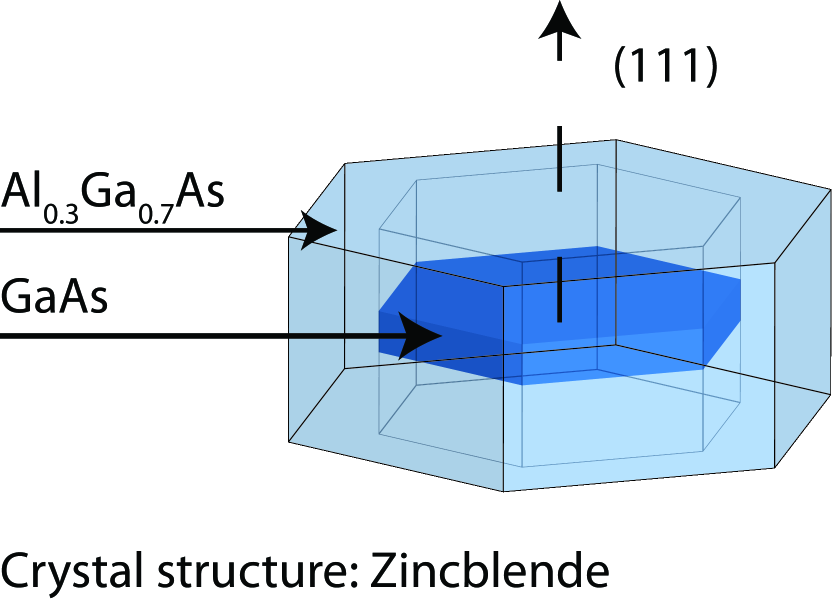
Figure 1: Schematics of a GaAs quantum dot within an Al_0.3Ga_0.7As nanowire

The true QD symmetry is the common symmetry of the mesoscopic heterostrocture and the microscopic crystal structure. The mesoscopic structure (Fig. 1) is symmetric (i.e. invariant) under discrete $\pm 2\pi/6$ rotations and under mirror operations w.r.t the six vertical planes containing the rotation axis, as well as w.r.t. the horizontal plane orthogonal to the rotation axis. These symmetry operations and their compositions form a point group of 24 elements called D${}_{\textrm{6h}}$ Altmann and Herzig (1994). Mathematically, the mesoscopic symmetry restriction on the conduction band Hamiltonian is expressed by the invariance relation pertaining to the confinement potential and effective mass appearing in Eq. II.1:

$$\left.\begin{array}[]{c}V_{\text{cb}}(\mathbf{r})=V_{\text{cb}}(\mathcal{R}(g)^{-1}\mathbf{r})\\ m^{*}(\mathbf{r})=m^{*}(\mathcal{R}(g)^{-1}\mathbf{r})\end{array}\right\}\forall g\in\textrm{D${}_{\textrm{6h}}$}.$$ (III.1)

Here, $\mathcal{R}$ is a set of standard representation matrices operating in 3D space Messiah (1959); Dalessi and Dupertuis (2010), and $\mathcal{R}(g)$ represents change of coordinates indexed by the group element $g$. The symmetry of our conduction band Hamiltonian (Eq. II.1) is then directly given by the mesoscopic symmetry D${}_{\textrm{6h}}$.

For the valence band, there are similar invariance constrictions due to the mesoscopic symmetry on $V_{\textrm{vb}}(\mathbf{r})$, and also on the spatially dependent Luttinger parameters $\gamma_{i}(\mathbf{r})$ (appearing in the $p,q,r,s$ polynomials)

$$\left.\begin{array}[]{c}V_{\textrm{vb}}(\mathbf{r})=V_{\textrm{vb}}(\mathcal{R}(g)^{-1}\mathbf{r})\\ \gamma_{i}(\mathbf{r})=\gamma_{i}(\mathcal{R}(g)^{-1}\mathbf{r}),i=1,2,3\end{array}\right\}\forall g\in\textrm{D${}_{\textrm{6h}}$}.$$ (III.2)

However, the valence band Luttinger Hamiltonian (Eq. II.3) also carries a face centered cubic diamond $O_{h}$ symmetry due to the underlying crystal, contained within the first term of Eq. II.3. When the orientation of the crystal axes w.r.t the mesostructure is as in Fig. 2, the common symmetry elements are those of the group C${}_{\textrm{3v}}$, i.e. $\{e,C_{3}^{+},C_{3}^{-},\sigma_{v1},\sigma_{v2},\sigma_{v3}\}$. Here $C_{3}^{+}$ and $C_{3}^{-}$ are discrete $2\pi/3$ rotations and $\sigma_{vi},i=1\ldots 3$ are three vertical mirror operations shown in Fig. 2. Hence the valence band Hamiltonian (Eq. II.3) has only C${}_{\textrm{3v}}$ symmetry. In the following we will therefore use the C${}_{\textrm{3v}}$ group as the main reference when introducing the necessary group theory concepts.

Description of the group, including group multiplication tables and group representations can be found in reference books like AltmanAltmann and Herzig (1994). For the single group C${}_{\textrm{3v}}$ there are three irreducible representations (irreps), $E$, $A_{1}$ and $A_{2}$. The $E$ irrep is a 2D representation whilst the $A_{i}$ irreps are 1D.

So far we have just considered the single group, describing operations performed on the spatial coordinates. The spinorial nature of the conduction and valence band does however necessitate the use of a double group representation. In the C${}_{\textrm{3v}}$ double group there are two 1D irreps ${}^{1}E_{3/2}$ and ${}^{2}E_{3/2}$ and one 2D irrep $E_{1/2}$. Altmann and Herzig (1994). With spin a change of the spatial coordinates $\vartheta(g)^{(3D)}$ ($\vartheta(g)^{(3D)}$ is an abstract functional operation corresponding to the change of coordinates described by the matrix $\mathcal{R}(g)$) should be accompanied by a corresponding change in spin space, $\vartheta(g)^{(j)}$. Such composite operations are thus defined by $\vartheta(g)=\vartheta(g)^{(3D)}\otimes\vartheta(g)^{(j)}$, where $\otimes$ is the tensor product between both operator spaces, and $g$ becomes an element of the double group. A natural choice for a standard representation of rotations in spinorial space in terms of Euler angles, $g\equiv(\alpha,\beta,\gamma)$, is the set of 4x4 Wigner matrices, $W(\alpha,\beta,\gamma)$Messiah (1959), since the Luttinger Hamiltonian is usually expressed in a Bloch function basis transforming like angular momentum and indexed $\left|{j,m}\right>$, $j=3/2$, where $m$ is the component along some quantization axis. Any matrix for improper rotation (i.e. mirror operations) can be obtained as a combination of proper rotations and spatial inversion, $i$, but since the diamond crystal structure is even under $i$, this can be ignored.

To fully take advantage of the symmetry properties of the valence band Hamiltonian, a specific choice of the Bloch basis is needed Dalessi and Dupertuis (2010). For some low symmetry groups, an optimal quantization axis can be found Dalessi and Dupertuis (2010), enabling full depth symmetry analysis. However, as explained in Ref. 1, in general a rotation of the quantization axis is not sufficient, and a more general unitary transformation of the basis has to be performed. The elements of the optimum basis are called Dalessi and Dupertuis (2010) Heterostructure Symmetrized Bloch Functions (HSBF’s), and are labeled by irreps of the double group.

The HSBF’s are symmetrized superpositions of the usual Bloch functions. For our C${}_{\textrm{3v}}$ Hamiltonian, the expressions for the HSBF’s are given by Eqs. B.7 and B.8 of App. B. The HSBF basis is written in terms of them as

$$\{\left|{{}^{1}E_{3/2}}\right>,\left|{E_{1/2},1}\right>,\left|{E_{1/2},2}\right>,\left|{{}^{2}E_{3/2}}\right>\}.$$ (III.3)

The ordering in Eq. III.3 is important to preserve the form of the time reversal symmetry operator Dalessi et al. .

Note that our choice of axes (Fig. 2) differs from that of Refs. 1; 24, in which the $z$-axis in the equations for the HSBF’s pertain to a quantization axis in the crystal direction $[\bar{1}10]$, i.e. corresponding to the $y$-axis in our present choice of coordinates. We have rather chosen the $z$-axis based on the special axis of the nanostructure ([111]), as the appropriate concept of light hole (LH) and heavy hole (HH) for our structure relates to $m_{z}=\pm\frac{1}{2}$ or $m_{z}=\pm\frac{3}{2}$ respectively for a $z$-axis along [111].

In the HSBF basis, the $p,q,r,s$ polynomials appearing in Eq. II.3 are given by

$$p=-\frac{1}{2}\left(\frac{\partial}{\partial{x}}\gamma_{1}\frac{\partial}{\partial{x}}+\frac{\partial}{\partial{y}}\gamma_{1}\frac{\partial}{\partial{y}}+\frac{\partial}{\partial{z}}\gamma_{1}\frac{\partial}{\partial{z}}\right)$$ (III.4a)

$$q=\frac{1}{2}\left(-\frac{\partial}{\partial{x}}\gamma_{3}\frac{\partial}{\partial{x}}-\frac{\partial}{\partial{y}}\gamma_{3}\frac{\partial}{\partial{y}}+2\frac{\partial}{\partial{z}}\gamma_{3}\frac{\partial}{\partial{z}}\right)$$ (III.4b)

$$r=-\frac{\partial}{\partial{x}}b\frac{\partial}{\partial{x}}+\frac{\partial}{\partial{y}}b\frac{\partial}{\partial{y}}-\frac{\partial}{\partial{z}}a\frac{\partial}{\partial{x}}-\frac{\partial}{\partial{x}}a\frac{\partial}{\partial{z}}$$ (III.4c)

$$s=-\frac{\partial}{\partial{y}}a\frac{\partial}{\partial{z}}-\frac{\partial}{\partial{z}}a\frac{\partial}{\partial{y}}+\frac{\partial}{\partial{x}}b\frac{\partial}{\partial{y}}+\frac{\partial}{\partial{y}}b\frac{\partial}{\partial{x}}$$ (III.4d)

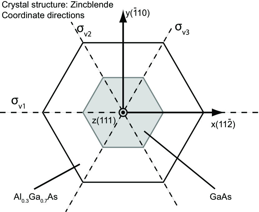
Figure 2: Coordinate axes and crystal directions for the hexagonal QD.

$$a=\frac{\epsilon}{2}\left(-\gamma_{3}-i\sqrt{2}\gamma_{2}\right)$$ (III.5a)

$$b=\frac{i\epsilon}{2}\left(\gamma_{2}+i\sqrt{2}\gamma_{3}\right)$$ (III.5b)

with $\epsilon=\frac{1-i\sqrt{2}}{\sqrt{3}}$. These expressions have been obtained by using the bulk expressions, e.g. by taking the Luttinger Hamiltonian expressed in direction [111] in Ref. 22, then changing its basis to the HSBF given in LABEL:{app:dsh_hsbf}, and finally by replacing $k_{j}\to-i\frac{\partial}{\partial{j}}$ for $j=x,y,z$.

In the forthcoming analysis, it will be useful to describe the spinorial nature of the quantum states using the concept of light hole (LH) and heavy hole (HH) dominant character (because of bandmixing the HH and LH states are mixed). Raw approximations for the effective masses parallel and perpendicular to the [111] axis can be read from Eqs. III.4a and III.4b (assuming $r$=$s$=0), and are given by

$$m^{*}_{||}=\frac{1}{\gamma_{1}\mp 2\gamma_{3}}$$ (III.6a)

$$m^{*}_{\perp}=\frac{1}{\gamma_{1}\pm\gamma_{3}},$$ (III.6b)

where the upper and lower sign applies to HH and LH respectively. For a normalized state $\left|{\psi}\right>$, the weight of the LH contribution is defined by

$$w^{[111]}_{LH}(\psi)\equiv\left|{}_{z}\langle 3/2,1/2|\psi\rangle\right|^{2}+|_{z}\langle 3/2,-1/2|\psi\rangle|^{2},$$ (III.7)

and similarly for the HH, so $w^{[111]}_{LH}+w^{[111]}_{HH}=1$. Using the basis change between the HSBF basis and the basis with quantization axis $[111]$, it is easy to show that

$$w^{[111]}_{LH}(\psi)=\left|\left.\left<{E_{1/2},1}\right|\psi\right>\right|^{2}+\left|\left.\left<{E_{1/2},2}\right|\psi\right>\right|^{2}.$$ (III.8)

We thus note that LH/HH character w.r.t. [111] is conveniently in one to one correspondence with $E_{1/2}/^{i}E_{3/2}$ character in the C${}_{\textrm{3v}}$ HSBF.

IV Symmetry implications on nanowire quantum dot states

The HSBF basis allows to maximally symmetrize the envelope functions appearing in the valence band spinors, and to give interpretation of the spinors as dominant product states. These possibilities, which are consequences of symmetry, are explored in the forthcoming subsections.

IV.1 Symmetry of envelope functions

We first recall the transformation properties of the double group spinors, in order to study the properties of envelope functions occurring in our nanowire QD. This is based on the MSRF techniqueDalessi and Dupertuis (2010). The HSBF-transformed Wigner matrices are denoted by $V^{B}(g)$, as they are block matrices in this basisDalessi and Dupertuis (2010). Indeed, one can write them as a direct sum, ${}^{1}E_{3/2}\oplus E_{1/2}\oplus^{2}E_{3/2}$, of the irrep matrices of the C${}_{\textrm{3v}}$ double group Dalessi and Dupertuis (2010). Therefore the spinor transformation (passive point of view), under any double group operation $g$, can then be written as

$$\left[\uline{\psi}(\mathbf{r})\right]^{\prime}_{j}=\left[\vartheta(g)\uline{\psi}(\mathbf{r})\right]_{j}=\sum_{k}[V^{B}(g)]_{j,k}[\uline{\psi}(\mathbf{\mathcal{R}}(g)^{-1}\bm{r})]_{k}.$$ (IV.1)

A seminal consequence of symmetry in a system subjected to invariance relations like Eqs. III.1 and III.2 is that it is always possible Hammermesh (1989) to label an eigenstate $\uline{\psi}$ by an irrep, $\Gamma$, and a partner function index, $\mu$ of the symmetry group, such that its corresponding transformation law is also:

$$\vartheta(g){\underline{\psi}}^{{\Gamma}}_{\mu}(\mathbf{r})=\sum_{\nu=1}^{d_{{\Gamma}}}\left[D^{{\Gamma}}(g)\right]_{\mu,\nu}\underline{\psi}^{\Gamma}_{\nu}(\mathbf{r})$$ (IV.2)

where $D^{{\Gamma}}(g)$ is a set of representation matrices for $\Gamma$, and $d^{\Gamma}$ is the dimension of $\Gamma$. For $D^{{\Gamma}}(g)$ we shall use the matrices of Refs. 1; 27, which correspond to a transposed multiplication table w.r.t. Ref. 26 since we use the passive point of view.

It is clear that Eqs. IV.1 and IV.2 strongly constrain the envelope function shapes, and it was shown in Dalessi and Dupertuis (2010) that they can be uniquely decomposed into ultimately reduced envelope function (UREF) components, transforming according to single group irreps. The classification of UREFs using single group labels could be used to reduce the computational domain significantly as argued in Ref. 1. We will see in the present work that it is also very helpful in the postprocessing and analysis of the data. In our QD, the full valence band spinors can be labeled by C${}_{\textrm{3v}}$ double group irreps, and expressed in terms of UREFs as in Eq. IV.3

$$\underline{\psi}^{{}^{1}E_{3/2}}=\left(\begin{array}[]{c}\phi^{A_{1}}\\ -\phi^{E}_{2}\\ \phi^{E}_{1}\\ -\phi^{A_{2}}\\ \end{array}\right)$$ (IV.3e)

$$\underline{\psi}^{{}^{2}E_{3/2}}=\left(\begin{array}[]{c}\phi^{A_{2}^{*}}\\ \phi^{E^{*}}_{1}\\ \phi^{E^{*}}_{2}\\ \phi^{A_{1}^{*}}\\ \end{array}\right)$$ (IV.3j)

$$\underline{\psi}^{E_{1/2}}_{1}=\left(\begin{array}[]{c}-\phi^{E}_{2}\\ \frac{1}{\sqrt{2}}[\phi^{A_{1}}+\Phi^{E}_{1}]\\ -\frac{1}{\sqrt{2}}[\phi^{A_{2}}+\Phi^{E}_{2}]\\ \varphi^{E}_{1}\\ \end{array}\right)$$ (IV.3o)

$$\underline{\psi}^{E_{1/2}}_{2}=\left(\begin{array}[]{c}\phi^{E}_{1}\\ \frac{1}{\sqrt{2}}[\phi^{A_{2}}-\Phi^{E}_{2}]\\ \frac{1}{\sqrt{2}}[\phi^{A_{1}}-\Phi^{E}_{1}]\\ \varphi^{E}_{2}\\ \end{array}\right).$$ (IV.3t)

The envelope functions have here been labeled in a simplified manner, keeping the double group labels of the global spinor and of the HSBFDalessi et al. implicit. The full labels should be restored for description of how the envelope functions of separate subequations in Eq. IV.3 transform into each other.

It should be pointed out that for QDs time reversal induces a unique mapping between Kramers degenerate spinors, in analogy to the $k\to-k$ mapping of quantum wires Dalessi et al. . The time reversal operator, $K$, is Dalessi et al. $K=FK_{0}$, where $K_{0}$, is a complex conjugate operator and $F_{j,k}=\delta_{k,(5-j)}(-1)^{j},\,\,(j,k)=1\ldots 4$. The 2D $E_{1/2}$ irrep is self conjugated, and the 1D irreps are mutually conjugated. Therefore, the pair of eigenstates belonging to a given eigenvalue is either the two partners of the self conjugated 2D irrep ($E_{1/2}$) or the pair of mutually conjugated 1D irreps (${}^{1}E_{3/2}$, ${}^{2}E_{3/2}$). Accordingly, $K\underline{\psi}^{{}^{1}E_{3/2}}=\underline{\psi}^{{}^{2}E_{3/2}}$ and $K\underline{\psi}^{E_{1/2}}_{2}=\underline{\psi}^{E_{1/2}}_{1}$. It is easy to see from the form of $K$ that the UREFs appearing in (IV.3e) must then be equal to the corresponding functions in (IV.3j). Similarly, for the ${E_{1/2}}$ irrep one obtains restrictions on (IV.3o) and (IV.3t):

$$\left.\begin{array}[]{l}\varphi^{E}_{i}={\phi^{E}_{i}}^{*}\\ \phi^{A_{i}}={\phi^{A_{i}}}^{*}\Rightarrow\textrm{$\phi^{A_{i}}$ is real}\\ \Phi^{E}_{i}=-{\Phi^{E}_{i}}^{*},\Rightarrow\textrm{$\Phi^{E}_{i}$ is imaginary}\end{array}\right\},\,\,\,i=1,2.$$ (IV.7)

In the scalar approximation, C${}_{\textrm{3v}}$ conduction band envelope functions can be given single group labels directly and states are either non-degenerate, $\Gamma=A_{i},i=1\ldots 2$, or twice degenerate, $\Gamma=E$. Accounting for spin, time reversal symmetry implies Kramers degeneracy and the eigenstates of the conduction band are either two-fold or four-fold degenerate. This also holds when one considers the full D${}_{\textrm{6h}}$ symmetry of the conduction band.

Having established in the present section the precise symmetry of every spinorial component using UREFs bearing single group irrep labels, we now propose to quantify the respective contributions of each irrep, assuming that the full spinors are all normalized to unity, i.e. $\left\|\uline{\psi}_{j}\right\|=1$.

The set of UREFs appearing in a given set $\uline{\psi}^{\Gamma}_{\mu}(\mathbf{r})$, transforming into each other according to $D^{\Gamma}(g)$ (of Eq. IV.2) are specified by $\psi^{\Gamma,\Gamma_{a}}_{\Gamma_{b},\mu_{a}}$. Here, $\Gamma_{b}$ label the relevant HSBF block and ($\Gamma_{a},\mu_{a}$) every individual UREF. There are internal redundancies within the UREFs due to their own transformation properties. We can define the weight of a subset of symmetry $\Gamma_{a}$ within the block $\Gamma_{b}$ of the spinor $\uline{\psi}^{\Gamma}_{\mu}$ (assuming that $\Gamma_{b}$ occurs only once in $\Gamma$) Gallinet et al. (2010):

$$w^{\Gamma_{b},\Gamma_{a}}\left(\uline{\psi}^{\Gamma}_{\mu}\right)=\left\|{\psi}^{\Gamma,\Gamma_{a}}_{\Gamma_{b}}\right\|$$ (IV.8)

is independent of $\mu$. In addition $\left\|{\psi}^{\Gamma,\Gamma_{a}}_{\Gamma_{b}}\right\|=\left\|{\psi}^{\Gamma,\Gamma_{a}}_{\Gamma_{b},\mu_{a}}\right\|$ is independent of $\mu_{a}$ by symmetryGallinet et al. (2010) (generalized Wigner-Eckart theorem); therefore partner function indices $\mu$ and $\mu_{a}$ are not relevant. With the chosen normalization, one of course has the completeness $\sum_{\Gamma_{b},\Gamma_{a}}d_{\Gamma_{a}}w^{\Gamma_{b},\Gamma_{a}}=1$. The redundancy by $d_{\Gamma_{a}}$ is because every UREF partner function contribute equal weight.

IV.2 Product states, dominant HSBF as DPGPS

In a $k\cdot{p}$ model, the global symmetry of the eigenstates of the heterostructure can always be expanded into sums of products between symmetrized scalar envelope functions labeled by single group $\Gamma$,$\mu$ (UREFs), and a HSBF labeled by double group $\Gamma$,$\mu$. Often, when band mixing is not too large, there is one dominant term in the expansion. One can infer that the first factor describes well the spatial probability distribution, and the second factor entails the symmetrized spin information encoded in the HSBF. In such a case we will denote the relevant HSBF the Discrete Point Group Pseudo Spin (DPGPS)Dupertuis et al. (2011). This notation express the fact that one can add such spinor parts in the same way as ordinary spin, but using the Wigner-Eckart theorem for point groups. Expressing the valence and conduction band states as such product states is often useful e.g. when building excitonic and biexcitonic complexes, and for simple understanding of degeneracies and other properties Dupertuis et al. (2011). As an example, consider an exciton with C${}_{\textrm{3v}}$ symmetry. Assume that the symmetry of the main electron states contributing to this exciton can be written as a direct product $\Gamma^{\textrm{electron}}=A_{1}\otimes{E_{1/2}}$. Similarly, assume that the symmetry of the hole states can be written as $\Gamma^{\textrm{hole}}=A_{1}\otimes\left({{}^{1}E_{3/2}\oplus^{2}E_{3/2}}\right)$. The excitonic states can then be constructed by combining separately the spinorial parts and the envelope parts. The symmetry of the excitonic states is thus $\Gamma^{\textrm{ex}}=\left(A_{1}\otimes{A_{1}}\right)\otimes\left({E_{1/2}}\otimes{\left({{}^{1}E_{3/2}\oplus^{2}E_{3/2}}\right)}\right)=2{E}$.

For the conduction band, writing the states as product states is straightforward. It is more complicated for the valence band, as band mixing may prevent a description of the states in terms of individual DPGPS. In the HSBF basis it is however easy to test the weight of every UREF part appearing in Eq. (IV.3) with the help of projection operators for scalar functions (on single group irreps) and calculating the weight (Eq. IV.8) of every individual component. We shall see that it often leads to interpretation of the nature of the eigenstates as product states of a dominant envelope function with a corresponding DPGPS. For example an ${}^{1}E_{3/2}$ state (IV.3e) with the dominant weight in the first ($A_{1}$) component, corresponds to the product state $\Gamma^{\textrm{hole}}=A_{1}\otimes^{1}E_{3/2}$.

One last comment regarding the DPGPS and its relationship with the HH/LH concept: as explained in Sec. III, in C${}_{\textrm{3v}}$ the HH-weight equals the combined weight of the two $E^{i}_{3/2}$ spinor components. The valence band state of the previous example (typically our QD ground state) may therefore be classified as HH-like. As shown in App. C the two corresponding "spin states" are distinct conjugated DPGPS in C${}_{\textrm{3v}}$, and to the two partners of $E_{3/2,g}$ DPGPS in D${}_{\textrm{6h}}$. Similarly LH-like spin states will be associated to the partners of $E_{1/2}$ DPGPS in C${}_{\textrm{3v}}$ and to those of $E_{1/2,g}$ DPGPS in D${}_{\textrm{6h}}$.

V Postsymmetrization

Postsymmetrization has been first demonstrated by Gallinet et al. using projection operators Gallinet et al. (2010). We will now present the PTCO, a novel systematic and streamlined postsymmetrization method developed to disentangle and classify numerical eigenstates such that they can be given individual symmetry labels. The advantages of the PTCO are: 1) that it can be used in combination with possibly existing calculation code for the electronic structure, so that little additional numerical/theoretical work is necessary (it is general and not limited to $k\cdot{p}$ theories). 2) That it will allow to test and qualify possible approximate elevated symmetries. We stress again that though these techniques are here exemplified starting from a simple 4 band $k\cdot{p}$ model, the PTCO can equally well be applied in the frame of more complex models.

For postsymmetrization, one considers a subspace of the space spanned by the set of eigenstates of the Hamiltonian. This subspace $\mathcal{S}$ of dimension $d_{\mathcal{S}}$ is obtained after selection of a few relevant eigenstates, $\{\uline{\psi}_{j},j=1\ldots d_{\mathcal{S}}\}$, which are numerical solutions of Eq. II.1 or Eq. II.3. It will be called the solution space. Usually we shall retain a finite set of neighboring eigenstates, from the ground state to a given maximum energy, e.g. $d_{\mathcal{S}}$=20 in Sec. VI. We shall assume that the states $\uline{\psi}_{j}$ are not entirely as symmetric as they should be (due to numerical errors or due to the use of a non-symmetric grid). Postsymmetrization techniques will aim at finding the best symmetrized states that can be found in $\mathcal{S}$, on the basis of the ideal symmetry properties that such linear combinations should satisfy.

For any operator, $F$, there is a matrix representation in $\mathcal{S}$, called $O(F)$, defined as

$$O(F)_{i,j}=\left.\left<{\uline{\psi}_{i}}\right|F\uline{\psi}_{j}\right>.$$ (V.1)

In the following subsections all operators, including the Hamiltonian $H$, the symmetry operators $\vartheta(g)$, the projection operators $P^{\Gamma}_{\mu}$, and the class operators $C_{i}$, will be identified with their matrix representation in $\mathcal{S}$.

Note that in the general case numerical eigenstates do not exactly obey Eq. IV.2 and they can be mixed in two ways. First, mixing can be due to fundamental degeneracy and the arbitrary choice of basis by the solver within every eigenspace. This effect can be strong but is not in violation of the symmetry of the (analytical) Schrödinger equation. Disentanglement is however necessary to enable the use of individual group labels corresponding to standard irreps $D^{\Gamma}(g)$ and belonging partner function indices $\mu$. Second, eigenstates can be mixed due to numerical inaccuracies, in particular if the grid does not respect the symmetry. Such mixing is always weak, when good convergence is achieved. If energy levels are closely spaced, symmetry breaking due to the grid may nevertheless couple states at nearby energies and with different symmetries. The goal of the PTCO, which is a global postsymmetrization method, is to disentangle both kinds of mixing simultaneously and it will be presented after a short description of a more standard technique based on projection operators.

V.1 Postsymmetrization using projection operators

A standard procedure to analyze and postsymmetrize the computed basis $\{\uline{\psi}_{j},j=1...d_{\mathcal{S}}\}$ is to use the a set of projection operators, $P_{\mu}^{\Gamma}$ which project any state onto the partner function $\mu$ of the irrep $\Gamma$. The projection operators are given by Hammermesh (1989)

$$P_{\mu}^{\Gamma}=\frac{d_{\Gamma}}{|\mathcal{G}|}\sum_{g\in\mathcal{G}}{\left({D^{\Gamma}(g)}_{\mu\mu}^{*}\vartheta(g)\right)}$$ (V.2)

where $|\mathcal{G}|$ is the number of elements of the group $\mathcal{G}$. A matrix representation in $\mathcal{S}$ can be built using Eq. V.1. The set of projection operators $P_{\mu}^{\Gamma}$ are orthogonal, and obeys

$$\sum_{\Gamma,\mu}P_{\mu}^{\Gamma}=1.$$ (V.3)

They can uniquely decompose any state into

$${\uline{\psi}=\left\{\sum_{\Gamma,\mu}P_{\mu}^{\Gamma}\right\}\uline{\psi}=\sum_{\Gamma,\mu}\uline{\psi}_{\mu}^{\Gamma}.}$$ (V.4)

The fact that the grid slightly breaks invariance will break the expected symmetry properties of the computed eigenstates $P_{\mu}^{\Gamma}\psi_{\mu^{\prime}}^{\Gamma^{\prime}}=\delta_{\Gamma,\Gamma^{\prime}}\delta_{\mu,\mu^{\prime}}\psi_{\mu}^{\Gamma}$. To quantify the amount of symmetry breaking for the basis functions of each double group irrep, we define the weight of $(\Gamma,\mu)$ in spinor $\uline{\psi}$ by

$$w^{\Gamma}_{\mu}\left(\uline{\psi}\right)=\left\|P_{\mu}^{\Gamma}\uline{\psi}\right\|.$$ (V.5)

For a perfectly symmetrized state $\uline{\psi}$, we have $w^{\Gamma}_{\mu}(\uline{\psi})\in\{0,1\}$.

The starting point for the standard postsymmetrization procedure is to compute the actual set of numbers $w^{\Gamma}_{\mu}(\uline{\psi}_{j}),j=1\dots d_{\mathcal{S}}$ for all ($\Gamma,\mu$), which give information on the symmetry content of any state. This information is used to identify subspaces where states of different symmetry have been mixed.

Then in a second step, symmetrized subspaces for all irreps can be built starting from a suitable set of representatives. Let $k$ be in this set, and let $w^{\Gamma}_{\mu}(\uline{\psi_{k}})$ be larger than the corresponding weight of the other irreps and other partner functions. The projected state $\uline{\overline{\psi}}^{\Gamma}_{\mu}=P^{\Gamma}_{\mu}\uline{\psi_{k}}/\left\|P^{\Gamma}_{\mu}\uline{\psi_{k}}\right\|$ transforming like $\Gamma,\mu$ is then a good starting point for the symmetrized subspace, the non-projective part of state $k$ is thrown away. For the 1D irreps e.g. ${}^{i}E_{3/2}$ this concludes the procedure, but for higher dimensional irreps like $E_{1/2}$ the remaining partner functions must be found to span fully every irrep subspace. One can then use transfer operators $T^{\Gamma}_{\mu\nu},\mu\neq\nu$, where $T_{\mu,\nu}^{\Gamma}=\frac{d_{\Gamma}}{|\mathcal{G}|}\sum_{g\in\mathcal{G}}{\left({D^{\Gamma}(g)}_{\mu\nu}^{*}\vartheta(g)\right)}$ (a generalization of Eq. V.2), and the property $\psi^{\Gamma}_{\mu}=T^{\Gamma}_{\mu,\nu}\psi^{\Gamma}_{\nu}$ to generate the basis.

Rather than the standard procedure, we propose below to use a global procedure, which do not throw away any information by selecting representatives. Here, all states will be taken into consideration in one step, rather than operating on every degenerate subspace sequentially. The procedure is not cumbersome, and it is easy to use. It does allow to automatically generate well behaved symmetrized eigenstates of the Hamiltonian.

V.2 Postsymmetrization using class operators

This procedure is based on the concept of commuting class operators, which are related to conjugation classes. The classes $\mathcal{C}_{i}$ of a group consist of elements that are conjugate to each other. Two group elements $g_{1}$ and $g_{2}$ of the group $\mathcal{G}$ are conjugate if there exists an element $g$ in $\mathcal{G}$ such that $g_{2}=g(g_{1})g^{-1}$.

Class operators are a set of operators $\{C_{i}\}$ constructed by summing operators corresponding to each element of a given class Chen (1989)

$$C_{i}=\sum_{g\in\mathcal{C}_{i}}\vartheta(g).$$ (V.6)

They are closed under multiplication and commute both with each other and with all group operations. These three properties make them useful e.g. in relation to the sought decomposition of the solution space into orthogonal symmetrized subspaces. The number of class operators equals the number of irreps of a group. This yields three classes for the C${}_{\textrm{3v}}$ group. One class consists of the identity, $\mathcal{C}_{e}=\{e\}$, one class of the three mirror operations, $\mathcal{C}_{\sigma}=\{\sigma_{vi},i=\ldots\}$, and the two rotation operations constitute the final class, $\mathcal{C}_{3}=\{C_{3}^{+},C_{3}^{-}\}$. The sought symmetrized basis vectors $\uline{\overline{\psi}}^{\Gamma}_{\mu}$ of $\mathcal{S}$ are eigenfunctions of the class operators. The class operator $C_{i}$ has eigenvalue $\lambda^{\Gamma}_{i}$, i.e. $C_{i}\uline{\psi}^{\Gamma}_{\mu}=\lambda^{\Gamma}_{i}\uline{\psi}^{\Gamma}_{\mu}$. This eigenvalue can be found directly from the character of the class, $\chi^{\Gamma}_{i}$; one hasChen (1989)

$$\lambda^{\Gamma}_{i}=\chi^{\Gamma}_{i}\frac{|\mathcal{C}_{i}|}{d^{\Gamma}}.$$ (V.7)

Here $|\mathcal{C}_{i}|$ is the number of elements in the class $\mathcal{C}_{i}$. Eq. V.7 can be used to deduce the group symmetry labels for the eigenfunctions directly without having to employ the projection operator.

The power of the class operators has been extensively described by ChenChen (1989). He showed in particular that the set of class operators linked with a canonical subgroup chain can be used to form a complete set of commuting operators (CSCO) for the group space. In our case, since we want a symmetrized basis in the solution space, we must add the Hamiltonian to have a CSCO, since the eigenvalue of the Hamiltonian will be sufficient to distinguish subspaces with identical symmetry. For our C${}_{\textrm{3v}}$ case, only one canonical subgroup is relevant, $C_{s}=\{e,\sigma_{v1}\}$. It will distinguish the partner functions belonging to the 2D irrep $E_{1/2}$. To this end we add the operation $\vartheta(\sigma_{v1})$, which is a class operator for $\mathcal{C}_{s}$. The CSCO in solution space is then:

$$CSCO=\{H,{C}_{3},{C}_{\sigma},\vartheta(\sigma_{v1})\}.$$ (V.8)

Here the trivial class operator $\mathcal{C}_{e}$ has been omitted since it corresponds to the identity.

The aim is to find symmetrized states which diagonalize the CSCO. It is then easier to combine all the CSCO operators into one single equivalent CSCO operator $C$ by forming

$$C=\alpha_{H}H+\alpha_{3}{C}_{3}+\alpha_{\sigma}{C}_{\sigma}+\alpha_{s}\vartheta(\sigma_{v1})$$ (V.9)

where the set of factors $\alpha$ must be chosen so that the eigenvalues of $C$ are non-degenerate. In the idealized case in which the states constituting the solution space are perfect eigenstates of $C$, non-degenerate $\alpha$’s would be sufficient. In practice one should however be careful when choosing the factors; guidelines for a good choice will be given in Sec. VI.4.

Let us now summarize the PTCO procedure. From the raw eigenvectors $\{\uline{\psi}_{j},j=1...d_{\mathcal{S}}\}$, a matrix representation is constructed for $C$ using Eq. V.1 and Eq. V.9. The contributing matrix representation for the Hamiltonian in this raw basis is just a diagonal matrix with the corresponding raw eigenvalues. The unitary matrix $V$, consisting of eigenvectors of $C$ will enable the diagonalization towards the diagonal matrix $\Lambda$

$$V^{\dagger}{C}V=\Lambda.$$ (V.10)

The matrix elements of $V$ provides in one automated run the new symmetrized eigenvectors (expressed in the new basis). Identifying the $k$-th symmetrized state as one of the sought symmetrized "eigenvectors" $\uline{\overline{\psi}}^{\Gamma}_{\mu,l}$, we get $V_{jk}=\left.\left<{\uline{\psi}_{j}}\right|\uline{\overline{\psi}}^{\Gamma}_{\mu,l}\right>$. The overbar stresses that in fact they are not anymore numerically perfect eigenvectors of $H$. Nevertheless, they are in a way more physical since part of their due symmetry, which was broken by numerics, has been restored by the procedure. The index $l$ was introduced to obtain a unique labeling, and is here usually chosen so as to number states with identical symmetry ($\Gamma,\mu$) by order of increasing energy. The symmetrized states can be easily constructed with

$$\uline{\overline{\psi}}^{\Gamma}_{\mu,l}=\sum_{j}\left.\left<{\uline{\psi}_{j}}\right|\uline{\overline{\psi}}^{\Gamma}_{\mu,l}\right>\uline{\psi}_{j}.$$ (V.11)

Having obtained a symmetrized basis, we must now identify the three labels $\Gamma,\mu,l$ for all states. The eigenvalues of $C$ can be discarded. It is much more informative to recompute the average values of the original CSCO (Eq. V.8), which will provide the labels for the symmetrized states. First,

$$\overline{E}^{\Gamma}_{\mu,l}=\left.\left<{\uline{\overline{\psi}}^{\Gamma}_{\mu,l}}\right|H\uline{\overline{\psi}}^{\Gamma}_{\mu,l}\right>$$ (V.12)

is nothing else than the new corrected energies. One notes the presence of the index $\mu$: the PTCO cannot restore completely the degeneracies lifted by the original numerical implementation. Nevertheless we still expect closely packed eigenvalues for each $\Gamma$, $l$ subspace. Second, the average values of the C${}_{\textrm{3v}}$ class operators are denoted

$$\overline{\lambda}^{\Gamma}_{i,\mu,l}=\left.\left<{\uline{\overline{\psi}}^{\Gamma}_{\mu,l}}\right|C_{i}\uline{\overline{\psi}}^{\Gamma}_{\mu,l}\right>$$ (V.13)

which are closely packed around the ideal value $\lambda^{\Gamma}_{i}$ Eq. V.7. Again there is a slight $\mu$ dependence. By comparison with Eq. V.7 one obtains the characters $\chi^{\Gamma}_{i}$ for every state, from which, via the character table, one can deduce the irrep $\Gamma$. Third, the corresponding value of the canonical subgroup class operator $\vartheta(\sigma_{v1})$ will provide the label $\mu$.

It is trivial to automate also the symmetry recognition step. Alternatively it can be performed using the projection operators Eq. V.2, with the advantage of giving a number which can be interpreted as a degree of symmetry, which is a figure of merit of the achieved symmetrization.

V.3 A hierarchy of symmetries

With the procedure we have developed, the numerical results will first be symmetrized w.r.t. C${}_{\textrm{3v}}$, constructing the CSCO given explicitly in the previous section. The C${}_{\textrm{3v}}$ symmetry is the true symmetry of the structure, only broken by the unsymmetric grid, and numerical errors. From the physical point of view, there might also be higher approximate symmetries like C${}_{\textrm{6v}}$, D${}_{\textrm{3h}}$ and D${}_{\textrm{6h}}$.

The C${}_{\textrm{6v}}$ symmetry group is constructed from C${}_{\textrm{3v}}$ by adding mirror operations w.r.t. three intermediate vertical symmetry planes ($\sigma_{di},i=1\ldots 3$), and D${}_{\textrm{3h}}$ is constructed from C${}_{\textrm{3v}}$ by inclusion of the mirror operation of the horizontal symmetry plane ($\sigma_{h}$). Combining the elements of C${}_{\textrm{6v}}$ and D${}_{\textrm{3h}}$ leads to the mesoscopic symmetry D${}_{\textrm{6h}}$. In both C${}_{\textrm{6v}}$ and D${}_{\textrm{3h}}$, there are three double group irreps, $E_{1/2},E_{3/2}$ and $E_{5/2}$, all two-dimensional. Their identical subduction tables to C${}_{\textrm{3v}}$ yields the correspondence $E_{3/2}\to^{1}E_{3/2}\oplus{}^{2}E_{3/2}$, $E_{5/2}\to E_{1/2}$ and $E_{1/2}\to E_{1/2}$. The subduction is similar for the D${}_{\textrm{6h}}$ group in which there are 6 similar double group irreps of gerade and ungerade type. The irrep matrices $D^{\Gamma}$ expanding the set given in Ref. Dalessi and Dupertuis (2010) are given for all groups in App. A.

We may investigate the validity of approximate symmetries by attempting to diagonalize a new CSCO constructed with respect to the elevated groups. In such a step, C${}_{\textrm{6v}}$, D${}_{\textrm{3h}}$ or D${}_{\textrm{6h}}$ class operators are included in the set of operators to be diagonalized. This implies choosing operators for the $\mathcal{C}_{6}=\{C_{6}^{+},C_{6}^{-}\}$ or the $\mathcal{S}_{3}=\{S_{3}^{+},S_{3}^{-}\}$ classes for C${}_{\textrm{6v}}$ and D${}_{\textrm{3h}}$, respectively Altmann and Herzig (1994). These operators enable distinction between $E_{1/2}$ and $E_{5/2}$ irreps. For D${}_{\textrm{6h}}$ we include both of them simultaneously.

One thus sees the versatility of the PTCO, which allows not only to restore the true symmetry, but also to investigate a possible hierarchy of symmetries as ever cruder, but informative, approximations to the problem at hand.

VI Numerical results

We consider a GaAs QD as described in Sec.II. The length of the hexagon edges is 20 nm and the axial length of the dot is 5 nm. An Al_0.3Ga_0.7As shell of thickness 10 nm surrounds the QD in the transverse direction, with infinite potential outside. In the axial direction, the dot is surrounded by a thick layer of Al_0.3Ga_0.7As, sufficient to ensure that all probability distributions goes to zero. The parameters utilized in the $k\cdot{p}$ Hamiltonian are summarized in Tab. 1.

Table 1: Parameters for $k\cdot{p}$ simulation, at 0K.

Effective el. mass Vurgaftman et al. (2001)	GaAs: $m^{*}=0.067$ AlAs: $m^{*}=0.15$
Luttinger Vurgaftman et al. (2001)	$\gamma_{1}$ $\gamma_{2}$ $\gamma_{3}$ GaAs: 6.9800 2.0600 2.9300 AlAs: 3.7600 0.8200 1.4200
Bandgap Vurgaftman et al. (2001)	$E_{g}^{GaAs}=1.519$ eV $E_{g}^{AlAs}=3.099$ eV $E_{g}^{Al_{x}Ga_{1-x}As}$ $=(1-x)E_{g}^{GaAs}+xE_{g}^{AlAs}-x(1-x)c$ $c=-0.127+1.310x$
Band offset	Ratio: 60.4:39.6 Yi et al. (2009) $E_{v}=0.396E_{g}^{Al_{x}Ga_{1-x}As}$ $E_{c}=0.604E_{g}^{Al_{x}Ga_{1-x}As}$

VI.1 Numerical implementation, convergence and accuracy

The potential is defined on a square grid using 91 points in the $x,y$ and $z$ direction, leading to the cross-section shown in Fig. 3. On the lateral sides wee see the deviation of the numerical implementation with respect to C${}_{\textrm{6v}}$ symmetry. Any effect from this symmetry breaking will later be ideally averaged by the PTCO.

To assess numerical convergence, we define the dimensionless numerical deviation $\Delta_{\text{num}}$. It is related to $\Delta_{E}$ which is the energy deviation relative to values obtained at highest resolution:

$$\Delta_{\text{num}}=\Delta_{\text{E}}\left(\frac{\hbar^{2}}{2m_{0}m^{*}}\frac{L_{\text{cd}}}{V_{\text{bar}}}\right)^{-1}.$$ (VI.1)

$V_{\text{bar}}$ is the potential difference between the dot and the first barrier, and $L_{\text{cd}}$ is a characteristic length of the computational domain, defined as the third root of the computational volume. For the valence band, $m^{*}$ is replaced by a directionally averaged HH mass (Eq. III.6). Using $\Delta_{\text{num}}$ to characterize the convergence allows to extrapolate by comparing the resolution dependence for the conduction and valence band.

Figure 4 shows $\Delta_{\text{num}}$ for valence band levels 1 and 15, and for conduction band levels 1 and 17 which contains similar dominant envelope functions. Only some low-resolution points are included for the computationally demanding valence band, confirming the convergence dependence. For a resolution of 91 points, we have $\Delta_{\text{num}}=1.25\cdot 10^{-8}$ for conduction band level 17. This corresponds to $\Delta_{E}=1.7meV$, and the corresponding extrapolated value for the valence band is -0.3 meV. Figure 4 also demonstrates that the relative energy differences within each band are more accurate than the absolute values.

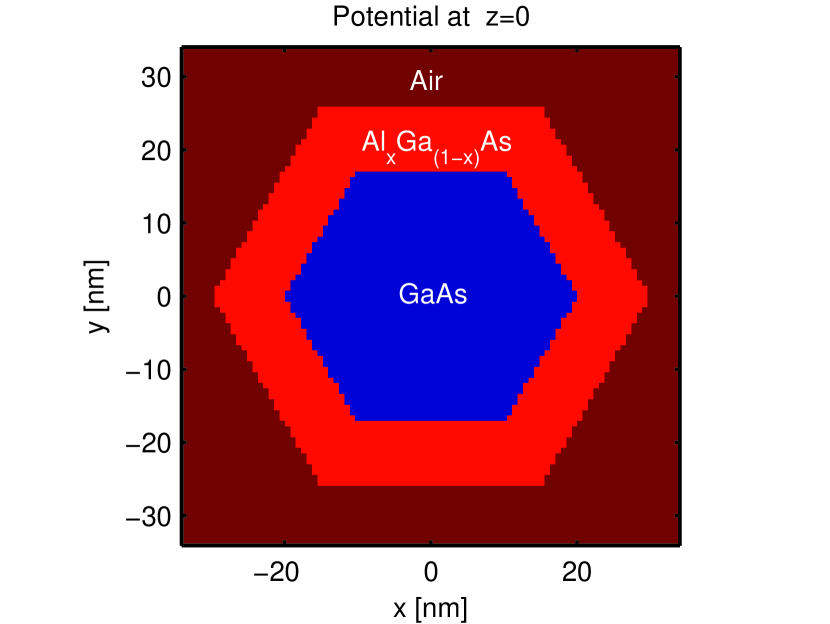
Figure 3: Cross section of the CB and VB potential in the transverse plane. Note the effect of the square grid on the lateral edges.

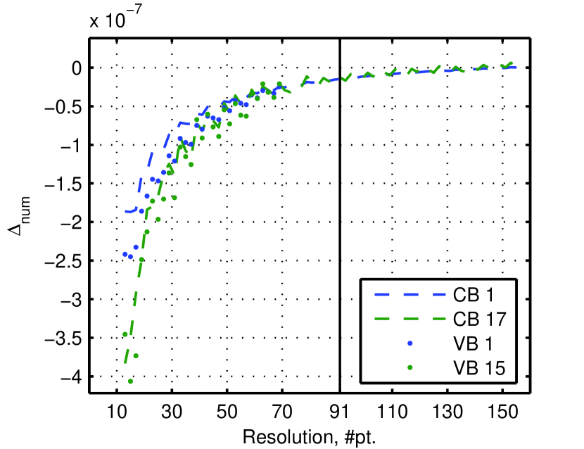
Figure 4: Numerical deviation $\Delta_{\text{num}}$ (dimensionless) for conduction band levels number 1 and 17, and for the valence band levels 1 and 15.

VI.2 Eigenenergies

The potential profile of the QD is shown in Fig. 5a). In Fig. 5b) we show the calculated lowest order energy levels for both electrons and holes. All energies are with respect to the top of the valence band. Note that the highest valence band level included here deviates from the top of the valence band by 39meV. In comparison, the split-off band is located a distance $\Delta_{\textrm{so}}=341$meV from the valence band top.

Figure 5: The potential profile along the axis of the nanowire (a), and the 10 or 15 lowest order energy levels of the conduction and valence band, respectively (b). All levels are twice degenerate due to time reversal. In Fig. 5 b), the CB levels marked with a dotted line correspond to $E$ states and are thus four-fold degenerate. Note that the energy scales are not equal.

VI.3 Conduction band eigenstates

Probability distributions $|\psi_{n}|^{2}$ for the 10 lowest levels in the conduction band are shown in Fig. 6. The full spinorial eigenfunctions $\uline{\psi_{n}}$ can be constructed from the scalar envelope functions $\psi_{n}$ Dalessi et al.

Since the states of the conduction band have the full D${}_{\textrm{6h}}$ symmetry in the present model, we label every envelope function in Fig. 6 by D${}_{\textrm{6h}}$ single group irreps. The D${}_{\textrm{6h}}$ irreps are labeled with subscripts $g$ and $u$, depending on whether they are even (gerade) or odd (ungerade) with respect to inversion. The gerade single group irreps are the 1D irreps $A_{1,g},A_{2,g},B_{1,g},B_{2,g}$, and the 2D irreps $E_{1,g}$ and $E_{2,g}$, similarly for the ungerade irreps($g\to u$). A complete summary of energies and symmetry labels is given later, in Tab. 6.

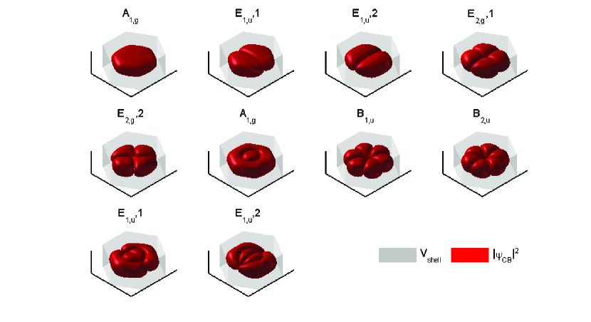
Figure 6: Isosurfaces of probability distributions, $|\psi_{\textrm{CB}}|^{2}$, for the conduction band states in order of increasing energy. Each state is twice degenerate due to spin. The barrier potential of the surrounding shell is $V_{\textrm{shell}}$. The D${}_{\textrm{6h}}$ single group symmetry labels are specified for each state. A detailed analysis, summarizing energy and symmetry properties, is given later in Tab. 6

.

VI.4 Valence band eigenstates

In the analysis of the valence band states, we will utilize extensively the PTCO outlined in Sec. V. First one needs to symmetrize the eigenstates w.r.t. the true C${}_{\textrm{3v}}$ symmetry of the original problem, as the small lack of symmetry due to the grid may strongly influence the choice of eigenstates within degenerate subspaces. The PTCO will also give quantitative information about the effect of the symmetrization process. In a second step we investigate approximate elevated symmetries with the same technique.

VI.4.1 Analysis of true C${}_{\textrm{3v}}$ symmetry

The combined CSCO operator, $C$, used for postsymmetrization according to C${}_{\textrm{3v}}$ is given by Eq. V.9; the $\alpha$ parameters were left free in Sec. V.2. From the numerical point of view, however, they must be chosen carefully to ensure well separated eigenvalues. To this end let us consider the eigenvalues of $C$. It is easy to show from the eigenvalue equation

$$C\overline{\uline{\psi}}^{\Gamma}_{\mu,l} = c^{\Gamma}_{\mu,l}\overline{\uline{\psi}}^{\Gamma}_{\mu,l}$$ (VI.2)

that one has

$$c^{\Gamma}_{\mu,l}=\alpha_{H}\overline{E}^{\Gamma}_{\mu,l}+\sum_{i=3,\sigma,s}\alpha_{i}\overline{\lambda}^{\Gamma}_{i,\mu,l}$$ (VI.3)

where $\overline{E}^{\Gamma}_{\mu,l}$ and $\overline{\lambda}^{\Gamma}_{i,\mu,l}$ are defined by Eqs. V.12 and V.13. The $c^{\Gamma}_{\mu,l}$ eigenvalues can be chosen freely, as they are directly related to the $\alpha_{k}$ coefficients. Since we know the ideal analytical eigenvalues $\lambda^{\Gamma}_{i}$ of the class operators Eq. V.7, and that the corrected energies $\overline{E}^{\Gamma}_{\mu,l}$ will be close to the original uncorrected energies it becomes possible to choose the $\alpha$ coefficients a priori in such a way that the CSCO eigenvalues $c^{\Gamma}_{\mu,l}$ will be well separated. To this end we consider the approximate spectrum of Eq. VI.3:

$$\tilde{c}^{\Gamma}_{\mu,l} = \alpha_{H}\overline{E}^{\Gamma}_{\mu,l}+\sum_{i=3,\sigma}\alpha_{i}\lambda^{\Gamma}_{i}+\alpha_{s}\lambda_{s,\mu}$$ (VI.4)

Note that we singled out the last parameter $\alpha_{s}$ which is related to the class operator of the subgroup $\mathcal{C}_{s}$ distinguishing different partner function indices $\mu$: to avoid confusion between $\lambda^{\Gamma}_{i}$ of C${}_{\textrm{3v}}$ and $\mathcal{C}_{s}$ we denoted the latter eigenvalue $\lambda_{s,\mu}$.

Since one of the eigenvalues may be chosen arbitrarily, it is convenient to shift $C$ by $\alpha_{H}E_{0}$, where $E_{0}$ is the ground state energy, and to make $c^{\Gamma}_{\mu,l}$ dimensionless by setting $\alpha_{H}=1/\max_{\Gamma,\mu,l}(\overline{E}^{\Gamma}_{\mu,l}-E_{0})$. One then obtains the set of eigenvalues

$$c^{\Gamma}_{\mu,l}=\frac{\overline{E}^{\Gamma}_{\mu,l}-E_{0}}{\displaystyle\max_{\Gamma,\mu,l}{\overline{E}^{\Gamma}_{\mu,l}-E_{0}}}+\tau^{\Gamma}_{\mu}$$ (VI.5)

such that the range of the energy splitting is normalized to unity. Here

$$\tau^{\Gamma}_{\mu}=\alpha_{s}\lambda_{s,\mu}+\sum_{i=3,\sigma}\alpha_{i}\lambda^{\Gamma}_{i}.$$ (VI.6)

The explicit choice of $\tau^{\Gamma}_{\mu}$ is given in Tab. 2, the $\alpha$’s can be easily obtained by inverting Eq. VI.6

Several considerations have been taken into account in our choice of $\tau^{\Gamma}_{\mu}$. In particular their relative magnitude decides which aspects are given highest priority. E.g. choosing $\tau^{\Gamma}_{\mu}\gg 1$ would emphasize very large separation w.r.t. group symmetry labels and enforce symmetry at the price of eventually remixing completely the Hamiltonian eigenstates. On the opposite, $\tau^{\Gamma}_{\mu}\ll 1$ would give negligible weight to symmetry considerations. We have chosen an intermediate set of values, where the relative step between neighboring energy levels are a bit smaller than the difference in eigenvalue for two functions belonging to different irreps. This choice was found appropriate for our structure, where the symmetry of degenerate states was slightly broken by a non-symmetric grid.

$\tau^{{}^{1}E_{3/2}}$	${\tau^{{}^{2}E_{3/2}}}$	$\tau^{E_{1/2,1}}$	$\tau^{E_{1/2,2}}$
-3.5	-1.5	0.5	2.5

Table 2: Parameters $\tau^{\Gamma}_{\mu}$ chosen to separate between C${}_{\textrm{3v}}$ irreps and partner functions

Having now determined the set $\alpha_{k}$, we computed the $C$ operator in a raw basis comprising the first 30 valence band states (including Kramers degeneracy) ordered by energy, and diagonalized it. To visualize the effect of mixing due to eigenstate symmetrization we plot in Fig. 7 the norm of the matrix elements of the unitary transformation matrix (Eq. V.11). Figure 8 display the change in energy $\Delta$E after symmetrization, confirming that the changes are modest.

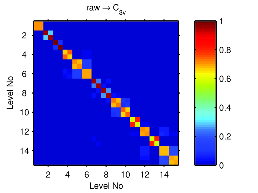
Figure 7: Norms of the matrix elements of the unitary transformation symmetrizing the eigenstates w.r.t. C${}_{\textrm{3v}}$.

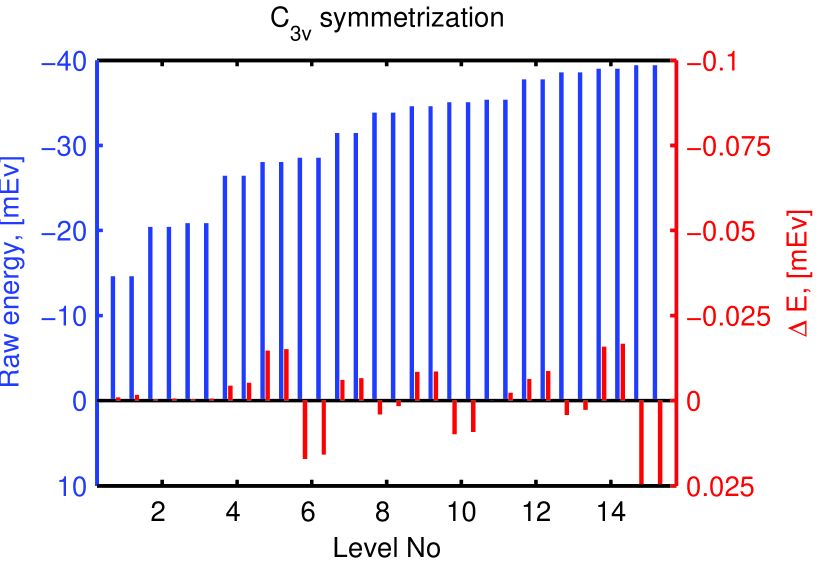
Figure 8: Changes in energies due to the symmetrization w.r.t. C${}_{\textrm{3v}}$. The raw energy spectrum is shown in blue, and the difference between the symmetrized and the raw spectrum is shown in red.

At large, the transformation matrix remixes states only within degenerate 2x2 subspaces corresponding to distinct Kramers doublets. There are no intertwined blocks, but the procedure would work even in this case, sorting correctly the partner functions and symmetrize them. In the raw states there were also some mixing between certain neighboring energy levels, as evidenced by the sequence of energies shown in Fig. 8. In this finer level one sees more subtle mixing extending over different Kramers doublets e.g. levels 5 and 6. This is a result of the nonsymmetric grid, and would be cumbersome to correct using a stepwise projection operator procedure rather than the automated PTCO. Such mixing increase for higher excited states, as expected. These include higher spatial frequencies, and will accordingly be more strongly influenced by limited grid resolution.

After symmetrization, we also analyze the C${}_{\textrm{3v}}$ irreps associated with different spinors. Fig. 9. shows the double group weight for the 30 lowest order states, divided again into 15 Kramers degenerate doublets. The eigenstates are very purely symmetrized w.r.t. C${}_{\textrm{3v}}$ ($w^{\Gamma}_{\mu}\left(\overline{\uline{\psi}}^{\Gamma}_{\mu}\right)\approx 1$), confirming the symmetry of the QD, and the postsymmetrization procedure. The small deviation for the highest order states is again due to grid inaccuracies. From Figs. 7, 8 and 9, we see that all the states that were most strongly symmetry mixed in the raw eigenspace did correspond to Kramers doublets with very small energy separation. However, there were also other off-diagonal mixing leading to the largest changes in energy.

We proceed to the analysis w.r.t. UREFs and single group irreps, which is shown in Fig. 10. The weights $w^{\Gamma}_{\mu}(\psi_{i})$, plotted for each HSFB component, $\psi_{i},i=1\ldots 4$ must be distinguished from the UREF weight $w^{\Gamma_{b},\Gamma_{a}}(\uline{\psi}^{\Gamma}_{\mu})$ defined in Eq. IV.8. Using Eqs. IV.8 and V.5 and Eq. (48) of Ref. 1, it is easy to see that they differ only by a Clebsch-Gordon coefficient:

$$w^{\Gamma_{a}}_{\alpha}(\psi^{\Gamma,\Gamma_{b}}_{\mu,\beta})=\left|C^{\Gamma,\Gamma_{b}^{*};\Gamma_{a}}_{\mu,\beta;\alpha}\right|w^{\Gamma_{b},\Gamma_{a}}(\uline{\psi}^{\Gamma}_{\mu})$$ (VI.7)

We use $w^{\Gamma}_{\mu}(\psi_{i})$ to be able to check the content of every HSBF component, in particular when it vanishes or when the weight is supposed to be equally distributed onto separate components. $w^{\Gamma}_{\mu}(\psi_{i})$ has easy interpretation, yielding directly the fractions of one given spinor component transforming according to the single group irreps. For the C${}_{\textrm{3v}}$ case, the two definitions differ by a factor $\sqrt{2}$ for the weight in the central components of the $E_{1/2}$ spinors, but the definitions are equivalent for the remaining UREFs.

Considering Fig. 10, we first note that the UREFs are in accordance with Eq. IV.3. However, there is a striking asymmetry between weights of partner functions 1 and 2 in the $\left|{{}^{i}E_{3/2}}\right>$ components of the $E_{1/2}$ states, most notably for levels 2 and 3 and 8 and 9. Due to time reversal symmetry, the two $\left|{{}^{1}E_{3/2}}\right>$ components and the two $\left|{{}^{2}E_{3/2}}\right>$ components, should correspond to partner functions of $E$ with the same weights. Such asymmetry can occur due to mixing of states from nearby energy levels if the states bear the same symmetry label. In this case, they are mixed in a way that cannot be sufficiently corrected by the C${}_{\textrm{3v}}$ symmetrization procedure. This explanation is supported by the fact that neighboring $E_{1/2}$ levels have opposite weight imbalance in Fig. 10, and also by their nearby energies in Fig. 8. We interpret such mixing as being a result of the imperfect grid and quasi-degeneracies. However, the presence of additional quasi-degeneracies should alert us of the possible existence of an approximate elevated symmetries, possibly able to correctly remix the relevant states.

Figure 9: Double group weights $w^{\Gamma}_{\mu}\left(\overline{\uline{\psi}}^{\Gamma}_{\mu}\right)$ w.r.t. the irreps of the C${}_{\textrm{3v}}$ group after C${}_{\textrm{3v}}$ postsymmetrization

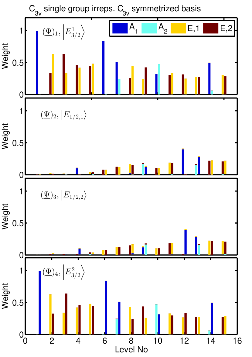
Figure 10: Single group weight $w^{\Gamma}_{\mu}\left(\overline{\psi}^{\Gamma}_{\mu}\right)$ with $\Gamma$, $\mu$ being single group irreps, for each spinor component in the HSBF basis after C${}_{\textrm{3v}}$ postsymmetrization.

VI.4.2 Analysis of elevated C${}_{\textrm{6v}}$ and D${}_{\textrm{3h}}$ symmetries

Figure 11: Double group weights w.r.t. the irreps of the elevated C${}_{\textrm{6v}}$ group. The eigenstates have been symmetrized w.r.t. the C${}_{\textrm{3v}}$ group.

The quasi-degeneracy of the first two $E_{1/2}$ levels hinted at the possible occurrence of approximate elevated symmetries. Such symmetries have previously been found both in theoretical Dalessi et al. and experimental Karlsson et al. (2010); Dupertuis et al. (2011) work on [111] oriented C${}_{\textrm{3v}}$ heterostructures. Because the mesoscopic structure has D${}_{\textrm{6h}}$ symmetry, we shall test the possible existence of C${}_{\textrm{6v}}$, D${}_{\textrm{3h}}$ and D${}_{\textrm{6h}}$ elevated symmetries to see if there is a hierarchy and, if so, how it is organized.

Fig. 11 show the weights of the C${}_{\textrm{3v}}$ symmetrized states according to irreps of the C${}_{\textrm{6v}}$ symmetry group. Very similar results were obtained for D${}_{\textrm{3h}}$. We see no change for ${}^{i}E_{3/2}$ states which are also well defined using these elevated symmetry groups. This is in agreement with the subduction table for C${}_{\textrm{6v}}$ to C${}_{\textrm{3v}}$ which yields $E_{3/2}{\to}E_{3/2}^{1}{\oplus}E_{3/2}^{2}$, the same applies for D${}_{\textrm{3h}}$. For the remaining irreps, the corresponding subduction yield $E_{5/2}{\to}E_{1/2}$ and $E_{1/2}{\to}E_{5/2}$. This is in accordance to the results of Figs. 9 and 11. However, we see clearly some irrep mixing which prevents unique labeling of these states in view of the elevated symmetry groups C${}_{\textrm{6v}}$ and D${}_{\textrm{3h}}$.

For closer investigation we shall perform a new symmetrization, as proposed in Sec. V. To this end, one extends the set of operators in the CSCO with class operators for classes of C${}_{\textrm{6v}}$ or D${}_{\textrm{3h}}$. This can be easily done by adding the operators of $\mathcal{C}_{6}$ or $\mathcal{S}_{3}$, respectively. There is no need to add further class operators for canonical subgroups here. This step allows to distinguish between the $E_{1/2}$ and $E_{5/2}$ irreps of the elevated groups. Of course one cannot expect the output of these elevated symmetrizations to be exact since they are not true symmetries of the QD. Our choice of symmetrization parameters is given in Tab. 3.

The parameters were again chosen to separate clearly the different irreps. Note however that the separation between $\tau^{\Gamma}_{\mu}$ for irreps that are indistinguishable in C${}_{\textrm{3v}}$ has been chosen smaller than the separation between those corresponding to different C${}_{\textrm{3v}}$ irreps, and also smaller than 1, giving the Hamiltonian priority over the approximate symmetry.

$\tau^{E_{3/2}}_{1}$	${\tau^{E_{3/2}}_{2}}$	$\tau^{E_{1/2}}_{1}$	$\tau^{E_{1/2}}_{2}$	$\tau^{E_{5/2}}_{1}$	$\tau^{E_{5/2}}_{2}$
-3.5	-1.5	0.65	2.65	0.35	2.35

Table 3: Parameters $\tau^{\Gamma}_{\mu}$ for symmetrization w.r.t. elevated symmetry groups C${}_{\textrm{3v}}$ and D${}_{\textrm{3h}}$.

We refer to the new eigenstates as C${}_{\textrm{6v}}$- and D${}_{\textrm{3h}}$- symmetrized, and denote the unitary transformation matrices from C${}_{\textrm{3v}}$ to C${}_{\textrm{6v}}$ by $V_{2}$, and from C${}_{\textrm{6v}}$ to D${}_{\textrm{3h}}$ by $V_{3}$. The norms of their matrix elements are shown in Fig. 12.

Figure 12: Norms of the matrix elements of $V_{2}$ and $V_{3}$, connecting the C${}_{\textrm{6v}}$-symmetrized and D${}_{\textrm{3h}}$-symmetrized states to C${}_{\textrm{3v}}$- and C${}_{\textrm{6v}}$- symmetrized bases respectively.

The transition from C${}_{\textrm{3v}}$ to C${}_{\textrm{6v}}$ (Fig. 12 a)) leaves the ${}^{i}E_{3/2}$ states practically unaltered, as expected from Fig. 11. These states were already well symmetrized by the basic C${}_{\textrm{3v}}$ symmetrization step. As expected we also see that quasi-degenerate subspaces that had $E_{1/2}$ symmetry in C${}_{\textrm{3v}}$ are now remixed, namely levels 2 and 3, 4 and 5 and also 8 and 9. Furthermore we see in the lower right corner of Fig. 12 a), three non-diagonal blocks mixing levels 11, 12 and 15 non-trivially together. The asymmetric structure of the intermixing blocks might indicate that a level above level 15 should also have been included in the solution space. Block structures like this are useful in revealing nearby states of similar symmetry.

Interestingly, symmetrization w.r.t. C${}_{\textrm{6v}}$ and D${}_{\textrm{3h}}$ have practically the same effect on the eigenstates. This is clearly seen in Fig. 12 b), showing the structure of the unitary transformation, $V_{3}$, between these two eigenstate bases. The main effect is merely an irrelevant reordering of some neighboring states. For this reason we shall not any more comment D${}_{\textrm{3h}}$ separately. Indeed the similarity of C${}_{\textrm{6v}}$ and D${}_{\textrm{3h}}$ indicate that D${}_{\textrm{6h}}$ symmetry will be the most relevant elevated symmetry.

It has still not been demonstrated that the elevated symmetry C${}_{\textrm{6v}}$ is in fact a good approximation to the true solution of the original Schrödinger equation. In Fig. 14, we show the variation of the energy levels due to the imposed symmetry C${}_{\textrm{6v}}$. One sees that the changes in energy remain very small ($\Delta E<0.6$ meV) compared to the confinement energies, confirming the continued validity of the Schrödinger equation. Not surprisingly, the alterations brought on by the elevated C${}_{\textrm{6v}}$ symmetrization does however lead to $\Delta E$ an order of magnitude bigger than for the C${}_{\textrm{3v}}$ symmetrization (Fig. 8). Clearly this is a manifestation that symmetries that are not true symmetries of the physical system are imposed. The C${}_{\textrm{6v}}$ symmetrization tend to bring closer energy levels with intermixed states. We also see that $\Delta E$ is biggest when non-degenerate subspaces are remixed, as expected.

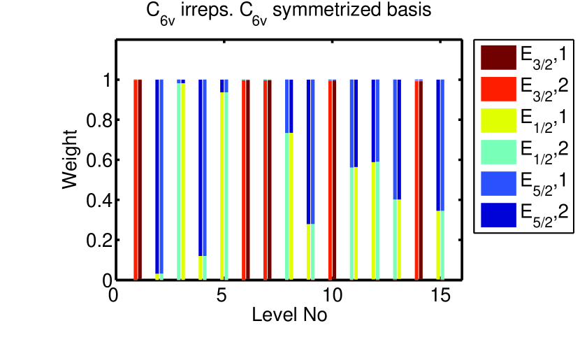
Figure 13: Double group weights $w^{\Gamma}_{\mu}(\overline{\uline{\psi}}^{\Gamma}_{\mu})$ of the irreps of the C${}_{\textrm{6v}}$ group after C${}_{\textrm{6v}}$ symmetrization of the basis.

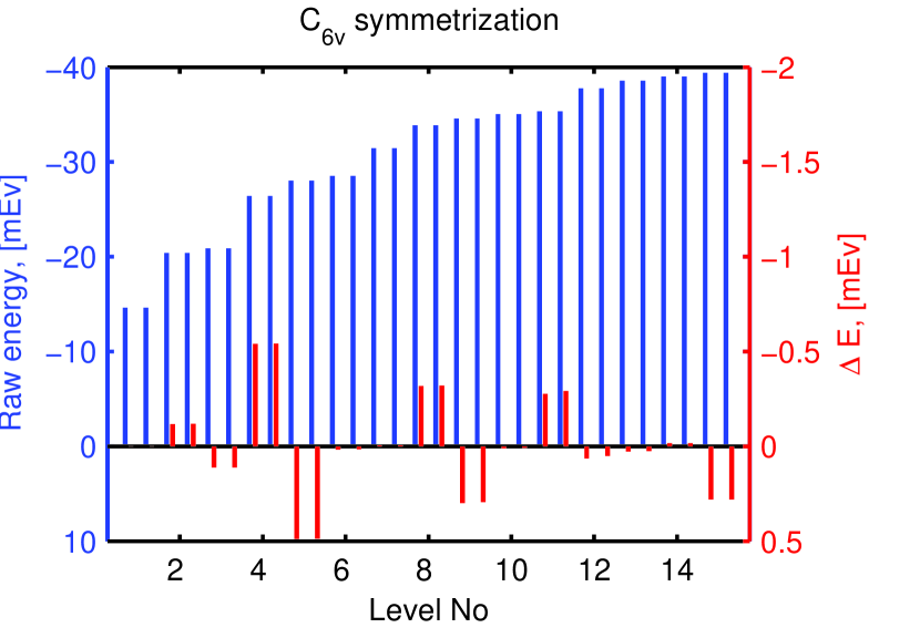
Figure 14: Changes in energies due to the symmetrization w.r.t. C${}_{\textrm{6v}}$ (very similar results hold for D${}_{\textrm{6h}}$ symmetrization). The raw energy spectrum is shown in blue, and the difference between the symmetrized and the raw spectrum is shown in red.

The weights of the C${}_{\textrm{6v}}$ double group irreps for C${}_{\textrm{6v}}$-symmetrized eigenstates are shown in Fig. 13. The identification of the C${}_{\textrm{6v}}$ double group irreps subduces correctly towards the previous identification with C${}_{\textrm{3v}}$ (Fig. 9). The most interesting aspect of Fig. 11 is certainly that the first two levels which were characterized by $E_{1/2}$ C${}_{\textrm{3v}}$ irreps (levels 2 and 3) are now distinct C${}_{\textrm{6v}}$ irreps, with nearly pure character, similarly for levels 4 and 5. As the two latter levels were not as much degenerate, their energy change is much larger (Fig. 8). The same comment also applies to levels 8 and 9, although we see that these levels do not seem to be well-described by the elevated symmetry. This is not surprising since states of higher energy levels are generally more sensitive to symmetry breaking contributions due to a microscopic structure. For the lower levels, the remixed states are well defined by $E_{1/2}$ or $E_{5/2}$ irrep labels, accordingly they approximately obey the symmetry of the elevated symmetry groups.

The symmetries of the spinor components of the C${}_{\textrm{6v}}$ symmetrized eigenstates are given in Fig. 15 (using only C${}_{\textrm{3v}}$ irreps, for easier comparison with Fig. 10). The single group decomposition of the components of the ${}^{i}E_{3/2}$ states obviously remains the same as in Fig. 10. It is more interesting to consider the $E_{1/2}$ states, especially those corresponding to levels 2 and 3, and also the states of levels 8 and 9. For these there is a meaningful difference. The weight imbalance present in Fig. 10 has essentially disappeared in the new eigenstate basis (Fig. 15). This is a proof that there was indeed a mixing between the quasi-degenerate levels due to grid imperfections that could not be retrieved by the C${}_{\textrm{3v}}$ symmetrization, since the involved states bared the same labels! In the elevated C${}_{\textrm{6v}}$ group, since mixed states bear different irreps they are easily disentangled. The restoration of the correct balance between the weights of partner UREFs bearing C${}_{\textrm{3v}}$ single group labels is also a clear signature of this fact.

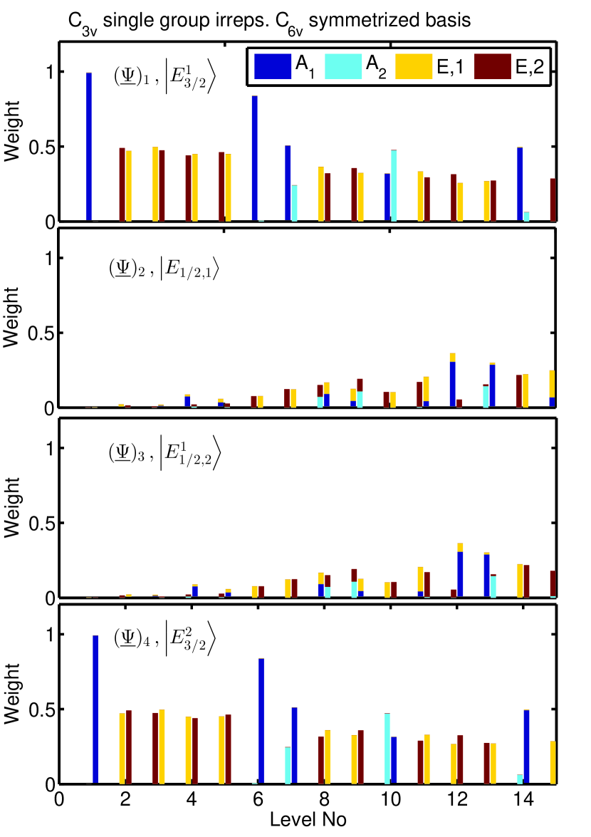
Figure 15: Weights $w^{\Gamma}_{\mu}(\overline{\psi}^{\Gamma}_{\mu})$ for each component of the HSBF basis, where $\Gamma$ $\mu$ are single group irreps and partner functions of the C${}_{\textrm{3v}}$ group. The eigenstates have been transformed using the C${}_{\textrm{6v}}$-symmetrization.

VI.4.3 D${}_{\textrm{6h}}$ as the ultimate elevated symmetry ?

The results from the symmetrization analysis in view of the elevated symmetries D${}_{\textrm{3h}}$ and C${}_{\textrm{6v}}$ revealed a very close relation between these symmetry elevations. This is a clear indication that the relevant elevated approximate symmetry group may in fact be D${}_{\textrm{6h}}$ which collects all the symmetry elements of D${}_{\textrm{3h}}$ and C${}_{\textrm{6v}}$. In fact this is not entirely surprising as the heterostructure symmetry is D${}_{\textrm{6h}}$, only broken at the microscopic level by the crystal symmetry which in principle does lower it to C${}_{\textrm{3v}}$. This motivates a symmetrization w.r.t. the D${}_{\textrm{6h}}$ symmetry, i.e. with inclusion of class operators for both $\mathcal{C}_{6}$ and $\mathcal{S}_{3}$ in the CSCO. The double group irreps of D${}_{\textrm{6h}}$ carry the same types of labels as C${}_{\textrm{6v}}$ and D${}_{\textrm{3h}}$, however there are twice as many as one has gerade and ungerade kinds. The $\tau^{\Gamma}_{\mu}$ parameters for the D${}_{\textrm{6h}}$ irreps are given in Tab. 4, the values for the gerade/ungerade were obtained by adding/subtracting 0.1 to the corresponding values in Tab. 3.

	$\tau^{E_{3/2,i}}_{1}$	${\tau^{E_{3/2,i}}_{2}}$	$\tau^{E_{1/2,i}}_{1}$	$\tau^{E_{1/2,i}}_{2}$	$\tau^{E_{5/2,i}}_{1}$	$\tau^{E_{5/2,i}}_{2}$
$i=g$	-3.6	-1.6	0.75	2.75	0.45	2.45
$i=u$	-3.4	-1.4	0.55	2.55	0.25	2.25

Table 4: Parameters $\tau^{\Gamma}_{\mu}$ for symmetrization w.r.t. elevated symmetry group D${}_{\textrm{6h}}$.

In Fig. 16 we first display the norm of the matrix elements of the unitary transformation bringing the C${}_{\textrm{6v}}$-symmetrized basis to the D${}_{\textrm{6h}}$ symmetrized basis. Except for levels 8, 9, 11, 12 and 15 there are little changes apart from trivial reordering of states. The remixing of the highest excited states cannot be analyzed due to the stringent limitation in the number of states kept in the solution space, but the remixing of levels 8 and 9 can be clearly interpreted as a further attempt to give distinct irreps $E_{3/2,u}$ and $E_{5/2,u}$ to these levels, that were not completely separated in the C${}_{\textrm{6v}}$ symmetrization ($E_{1/2}$ and $E_{1/2}$ in Fig. 11). We clearly see that the departure from D${}_{\textrm{6h}}$ symmetry, due to the underlying symmetry of the Zinc Blende lattice, starts to be important after level 10, in particular for levels 11,12 and 15 which have strongly mixed character with respect to D${}_{\textrm{6h}}$ symmetry.

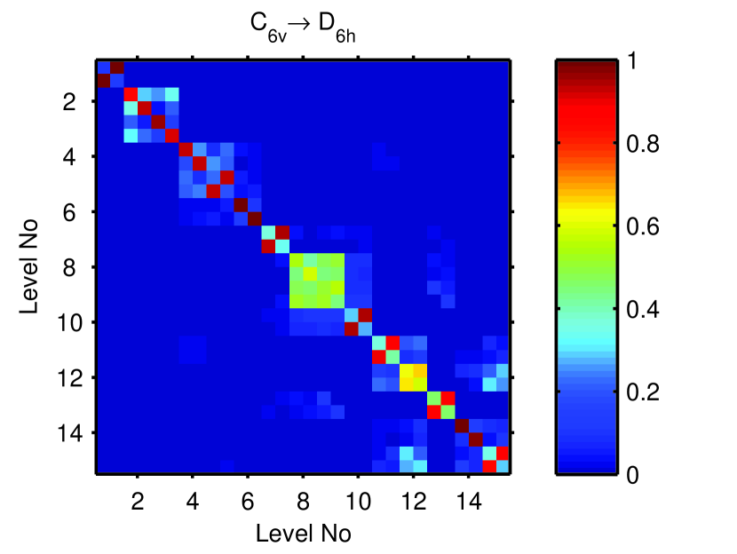
Figure 16: Unitary transformation between bases symmetrized w.r.t. C${}_{\textrm{6v}}$ and D${}_{\textrm{6h}}$ symmetries.

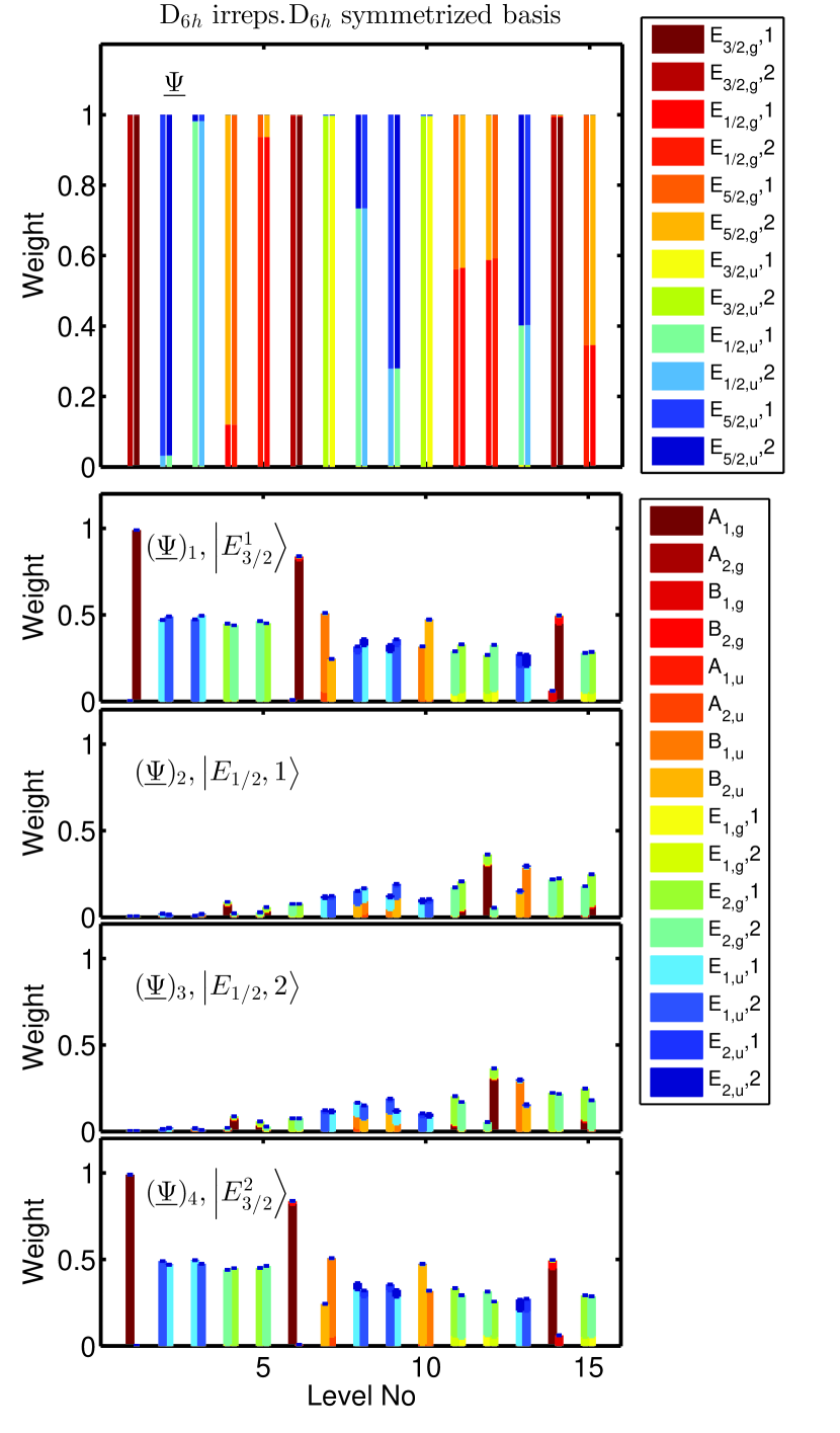
Figure 17: Double group weights and single group weights for each HSBF component w.r.t. D${}_{\textrm{6h}}$ group, using the D${}_{\textrm{6h}}$ symmetrized basis.

The energy changes $\Delta E$ due to the D${}_{\textrm{6h}}$ symmetrization are given in Tab. 5. From this we see again that neighboring levels bearing $E_{1/2}$ labels in view of C${}_{\textrm{3v}}$ are renormalized. The energy differences are very similar to the corresponding values for C${}_{\textrm{6v}}$ (Fig. 14). In Fig. 17a), we show the double group weights of the D${}_{\textrm{6h}}$-symmetrized eigenstates. The purities of the states w.r.t. the double group irreps displayed in Fig. 17a) are also very similar to the corresponding C${}_{\textrm{6v}}$ analysis (Fig. 11). The D${}_{\textrm{6h}}$ symmetry is thus fulfilled to approximately the same degree as the intermediate symmetries C${}_{\textrm{6v}}$ and D${}_{\textrm{3h}}$, as is also confirmed by the deviation in energy due to the D${}_{\textrm{6h}}$ symmetrization (Tab. 5), which stays on the same order as for C${}_{\textrm{6v}}$.

The single group analysis of each spinorial component in the HSBF basis in Fig. 17 b) leads to results in fair agreement with the UREFs for D${}_{\textrm{6h}}$ which are listed in App. C. These results fully confirm the relevance of the approximate symmetry elevation to D${}_{\textrm{6h}}$ for the valence band in our structure, and clearly shows when it applies and when it has limitations. In the following section a more in depth analysis of the UREF weights of Fig. 17 is carried out.

VI.5 Characterization of DPGPS, UREF’s and envelope function symmetry of valence band eigenstates

Up to now we have concentrated on the symmetry properties of eigenstates as a whole. It is however possible to get important information and insight within each of them by studying the nature of the UREFs, identifying dominant HSBF (DPGPS) and dominating UREF. Such an approach will not only provide enhanced physical interpretation and intuition, but can also reveal to be extremely helpful information when building more complex objects, e.g. multiexcitons in a configuration interaction approach and in the strong confinement limit (c.f. 31; 35).

The analysis will be carried out using essentially elevated D${}_{\textrm{6h}}$ symmetry which provides the finest classification, establishing the DPGPS in Sec. VI.5.1 and determining the dominant UREF’s in Sec. VI.5.2. The analysis is finally completed in Sec. VI.5.3 by an analysis in terms of more classical azimuthal and radial quantum numbers, which provides an intuitive understanding for the sequence of irreps and outlines a link to symmetry adapted functions Altmann and Herzig (1994).

The main results of this section are summarized in Tab. 5. Together with Fig. 17, Tab. 5 provides a deep understanding of all valence band states which will allow to decipher the remarkable properties of the optical transitions.

VI.5.1 Heavy and Light hole mixing, HSBFs and DPGPS

The most common way to analyze valence band states in heterostructures is in terms of valence band mixing between HH and LH states. This is an import from quantum well physics where, at zone-center, there is no mixing. In strongly oblate (c.f. Fig. 1) disk-like structures this is still a good starting point due to weak mixing for the ground states, allowing to deduce that the ground state should be HH-like. Moreover one can predict further the order of excited HH- and LH-like states coarsely using a scalar anisotropic effective mass model based on Eqs. III.6 which neglects valence band mixing and assumes an infinite cylindrical potential well with the same height and cross sectional area as the nanowire QD. One obtains a separation of about 45 meV between the ground HH and LH states. Accordingly, we do expect the 15 lowest energy levels (Fig. 5) to be dominated by HH states, in agreement with what can be seen in Figs. 10 and 17, where it is easy to see that the HH-weight always remains above 0.5 using Eqs. III.7 and III.8. We also see clearly in Figs. 10 and 17 that the degree of bandmixing increases with increasing excitation levels, as expected. It is very low for the ground state, 99% HH, and starts to be significant above level 6.

We now proceed to identify the DPGPS, i.e. the dominating HSBF of a mixed state. Being HH-like, the DPGPS of all the first 15 Kramers conjugate pairs is $\left|{E_{3/2}^{i}}\right>,i=1,2$ in C${}_{\textrm{3v}}$, and the corresponding DPGPS in D${}_{\textrm{6h}}$ are the partners of $\left|{E_{3/2,g}}\right>$ (c.f. App. B).

The concepts of DPGPS and dominating UREF are important and will enable understanding of the quasi-degeneracies in the next section.

VI.5.2 Analysis of UREFs

Let us first identify for every level (Kramers’ pair) the dominant UREFs, using Fig. 17. We find the following dominances: level 1, 6 and 14 are $A_{1,g}$, levels 2, 3, 8, 9 and 13 are $E_{1,u}$, levels 4, 5, 11, 12 and 15 are $E_{2,g}$, level 7 is $B_{1,u}$ and level 10 is $B_{2,u}$. This is summarized in column 6 of Tab. 5, column 4 (for C${}_{\textrm{3v}}$) can be obtained by subduction. Note that we have already regrouped some levels together as pairs in this enumeration, the reason will become clear during the forthcoming analysis.

The concept of product states between the dominant UREF and DPGPS allows to explain most of the level sequence in Fig. 17. Indeed, the double group irrep of each level (or the irrep pair in case of a level pair) can be faithfully generated by making the following products of irreps: for the isolated levels 1, 6 and 14 $A_{1,g}\times E_{3/2,g}=E_{3/2,g}$, for the level pairs 2, 3 and 8, 9 $E_{1,u}\times E_{3/2,g}=E_{5/2,u}+E_{1/2,u}$, for level pairs 4, 5 and 12, 15 $E_{2,g}\times E_{3/2,g}=E_{5/2,g}+E_{1/2,g}$, for level 7 $B_{1,u}\times E_{3/2,g}=E_{3/2,u}$, for level 10 $B_{2,u}\times E_{3/2,g}=E_{3/2,u}$, for level 11 $E_{2,g}\times E_{3/2,g}=E_{1/2,g}$ ($+E_{5/2,g}$ but the latter is missing), and finally for level 13 $E_{1,u}\times E_{3/2,g}=E_{5/2,u}$ ($+E_{1/2,u}$ but the latter is missing). The missing levels related to level 11 and to level 13 likely lie above the 15th energy level. The association of level 12 (instead of 11) with level 15 will be explained in the next section when looking at azimuthal and radial quantum numbers. It is still an open question whether the departure from D${}_{\textrm{6h}}$ symmetry of levels 11, 12 and 15 may be further minimized by including the missing partner of 11 in the symmetrization procedure (c.f. Fig. 16).

The clustering in energy of the level pairs 2, 3 and 4, 5 and 8, 9, and 12, 15 (see Figs. 14 and 5) can also be very clearly explained by dominant product states. It should be kept in mind that the quasi-degeneracies of 4,5 and 12,15 with levels 6 and 13,14 respectively are accidental since these have different symmetries. Whilst the energy of the lower pairs are closely packed together due to negligible valence band mixing, higher pairs like 8, 9 and 12, 15 become more and more significantly split apart. The splitting is however already visible for the level pair 4, 5, manifested in Fig. 17 as non-vanishing weight in the central $E_{1/2}$ components in which there are distinct UREFs for the respective levels. This is a clear demonstration that band-mixing is also a very relevant concept in the HSBF picture.

The isolated levels 1, 6 and 14 are all linked with the dominating $A_{1,g}$ UREF. Although it is customary that the fundamental level is strongly dominated by a fully invariant envelope function concentrated in the DPGPS component, the structure of levels 6 and 14 can again only be explained in the next section when looking at azimuthal and radial quantum numbers. Note that level 14 also display contributions from other HSBF components.

Levels 7 and 10 are also interesting. They are very similar and in a way form a complementary pair because the relative strength of the weights of $B_{1u}$ and $B_{2u}$ is opposite between the two levels. In fact within one level none of the two is strongly dominant, but this is allowed by symmetry since the two products $B_{1,u}\times E_{3/2,g}$ and $B_{2,u}\times E_{3/2,g}$ give both of them global $E_{3/2,u}$ symmetry. In contrast with the partners of an $E_{1,u/g}$ or $E_{2,u/g}$ irrep (see Fig. 17) which must be always balanced as predicted by the Wigner-Eckart theorem, the weights of the $B_{1u}$ and $B_{2u}$ UREFs must not necessarily be balanced in these levels. Levels 7 and 10 therefore illustrate the general fact that even if a state has a clear DPGPS (clearly dominant HSBF) it may not necessarily have a single very dominant UREF, as allowed by the analytical UREF decompositions given in App. C.

Thus far we have only considered the DPGPS components of the spinors, however the higher excited levels also have a significant contribution from the $E_{1/2}$ HSBFs (LH). For simplicity we shall discuss this only in C${}_{\textrm{3v}}$ symmetry. First, note that all $E$-partner functions within LH components have balanced (equal) weight despite band mixing: this is imposed by symmetry (c.f. Eq. IV.3). By contrast, and in analogy to the discussion of the previous paragraph, level 13 has $A_{i},i=1,2$ UREF pairs in the LH components with an allowed weight imbalance. Second, we have seen analytically that time reversal symmetry imposes restrictions (c.f. Eq. IV.7) on the LH components of the $E_{1/2}$ states. As a clear example let us consider the first pair of $E_{1/2}$ states with significant LH weights, levels 8 and 9, which in addition contain all UREFs predicted by Eq. IV.3, as can be seen in Fig. 11. We have been able to check numerically that indeed the relative phase of the $A_{1}$ and $A_{2}$ UREFs are out of phase with the $E$ UREFs by a factor $i$ in agreement with Eq. IV.7. Note also that level 12 has a rather large $A_{1}$ LH component, we do not think however that this state should be identified with a ground LH-like state.

Finally, it is interesting to consider the parity of the dominant UREFs found with respect to the $\sigma_{h}$ operation. From the D${}_{\textrm{6h}}$ character table it is easy to see that all the single group irreps of the dominant UREFs appearing so far, namely $A_{1,g},A_{2,g},B_{1,u},B_{2,u},E_{2,g}$ and $E_{1,u}$ are even under $\sigma_{h}$ (nevertheless it should be noted that non-dominant UREFs may acquire some level of $z$ excitation due to bandmixing (c.f. Fig. 17)). The reason for this behavior of the dominant UREFs is rooted in the high lateral to axial aspect ratio of the QD under consideration which is 40:5 (c.f. Fig. 1). We therefore expect the envelope functions of the 15 lower levels considered here to have excitations mainly in the transverse plane (azimuthally and radially). This is investigated in the following subsection (Sec. VI.5.3).

To conclude we would like to stress that the dominant UREFs that we have identified in this subsection will play a key role not only in enabling the use of azimuthal and radial quantum numbers, but also in analyzing the strength of optical transitions.

VI.5.3 Approximate azimuthal and radial quantum numbers: the role of symmetry adapted functions

The goal of this section is to investigate the correspondence between a classical effective mass analysis for a disk-shaped quantum dot in terms of standard azimuthal and radial quantum numbers (as we have just seen there is no need for a vertical $n_{z}$ quantum number), and the sequence of irreps for the dominating UREFs identified in the previous section.

The Schrödinger equation for a circular disk-shaped QD with infinite barriers is separable in azimuthal and radial coordinates, and leads to eigenfunctions which are proportional to products of an azimuthal exponential $\exp(im_{a}\phi)$ with an $l_{a}$-th order Bessel function $J_{l_{a}}(k_{l_{a},n_{r}}r)$ for the radial coordinate, where it is understood that $k_{l_{a},n_{r}}R$ is the $n_{r}$-th zero of $J_{l_{a}}$ with $R$ being the dot radius. They are labeled by the azimuthal and radial quantum numbers, $l_{a}=0,1,\ldots,\infty$ and $n_{r}=1,\ldots,+\infty$. In cylindrical coordinates, $m_{a}$ is restricted to $m_{a}=\pm l_{a}$ (and axial excitations are labeled by $n_{z}$). The number of azimuthal nodes is thus $l_{a}$, and there is a twofold degeneracy for states with $l_{a}\neq 0$.

Similar approximate quantum numbers can be expected in our nearly cylindrical 3D solutions, see Fig. 6 for the conduction band, and Fig. 18 for the valence band spinor component cross sections. Therefore, in the following we shall specify the character of the computed dominating UREFs not only by their irreps, but also by additional subscripts $\psi^{\Gamma}_{n_{a},n_{r}}$ where $n_{a}$ and $(n_{r}-1)$ specify the number of nodes in azimuthal and radial direction respectively (when they can be determined). The subscripts were identified by visual inspection for the first 15 levels, and are listed in the last column of Tab. 5.

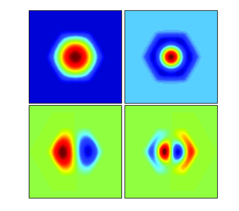
Figure 18: Cross sections of a selection of the contributions to the valence band spinor. The envelope functions shown in the top row are characterized as $\psi_{01}^{A_{1,g}}$ and $\psi_{02}^{A_{1,g}}$, in the order from left to right. The two functions in the lower row are $\psi_{11}^{E_{1,u},1}$ and $\psi_{12}^{E_{1,u},1}$.

We now consider the energy level sequences. First the sequence of levels 1, 6 and 14 with dominating UREF of $A_{1,g}$ symmetry: it is easy to see that they nicely form the sequence of $m_{a}=0$ levels with $n_{r}=1,2,3$, i.e. purely radial excitations.

Another less trivial, but fundamental, sequence is the $n_{r}=1$, $l_{a}=1\ldots 5$ sequence. We recognize the following five level pairs: 2 and 3, 4 and 5, 7 and 10, 11 and missing partner, 13 and missing partner. The question is now how to obtain further confirmation of this sequence. If one looks at the subduced representations from O(3), the so-called Symmetry Adapted Functions (SAFs), listed in Table T35.5 and T35.6 of Ref. 26, we can confirm that the link is correct, as the SAF quantum numbers $l,m,$ here corresponding to $l_{a},m_{a}$ are in agreement with the appropriate single group labels. One finds that the $l=1,m=\pm 1$ basis subduces to $E_{1,u}$ in D${}_{\textrm{6h}}$ symmetry, $l=2,m=\pm 2$ subduces to $E_{2,g}$, $l=3,m=\pm 3$ subduces to $B_{1,u}+B_{2,u}$, $l=4,m=\pm 4$ subduces to $E_{2,g}$, and finally , $l=5,m=\pm 5$ subduces to $E_{1,u}$. Hence we have confirmed that this sequence of azimuthal excitations is in agreement with the sequence of irreps for the dominating UREFs, and additionally that levels 11 and 13 have missing partners which must be at higher energies. For level 11, this was also indicated by the structure of the intermixing blocks in the lower right corner of Fig. 17 as previously mentioned.

Similarly we can identify the last $n_{r}=2$, $l_{a}=1,2$ sequence corresponding to level pairs 8, 9 and 12, 15. Again, the corresponding $l,m$ quantum numbers subduce to the correct irreps $E_{1,u}$ and $E_{2,g}$ respectively.

Even further interpretation is sometimes permitted. Let us consider again the pair of levels 7 and 10. Three nodal planes here correspond to either $B_{1,u}$ or $B_{2,u}$ symmetry. These are distinguished by a rotation by $\pi/6$ of the nodal planes. In our choice of coordinate system (Fig. 2), the $\psi^{B_{1,u}}_{31}$ functions have nodal planes perpendicular to the facets of the hexagon, whereas the $\psi^{B_{2,u}}_{31}$, have nodal planes intersecting the corners of the hexagon. These two orientations give rise to different filling factors. The $\psi^{B_{1,u}}_{31}$ functions fill the area of the hexagon more effectively than the corresponding functions with $B_{2,u}$ labels. The curvature, and thus the energy is therefore higher for the $\psi^{B_{2,u}}_{31}$. This is also seen in the conduction band, as there is a splitting between the two corresponding levels (CB levels 7 and 8). For the valence band, the spinors do in fact contain mixtures of $\psi^{B_{1,u}}_{31}$ and $\psi^{B_{2,u}}_{31}$. Energy level 7 has $B_{1,u}$ as the largest contribution and a smaller contribution of $B_{2,u}$. The situation in energy level 10 is mirrored. The energy splitting between the levels is mostly due to the different curvature of $\psi^{B_{1,u}}_{31}$ and $\psi^{B_{2,u}}_{31}$. Note that the different curvature of states rotated by $\pi/4$ also apply for the $E_{1}/E_{2}$ states with azimuthal excitations. However for these states unequal weight in the UREF partners would violate the restrictions from Wigner-Eckart theorem.

As valence band mixing is weak for the lowest energy levels, the corresponding dominant HH envelopes will not hybridize with LH components. The lowest order UREFs observed in the LH components are $\psi^{B_{i,u}}_{31},i=1..2$ envelope functions. This also further supports our previous assumption regarding the DPGPS as there is no sign of an LH-like sequence.

Note that the considerations of this section can also be carried out for the simpler conduction band, we leave this as an exercise for the reader. The situation in the valence band is much more complicated due to direction-dependent effective masses and valence band mixing. We expect that the approach also works when sequences of vertically excited states occur, and with $E_{1/2,g}$ DPGPS states (LH-like).

At this stage Table 5 entails the full information for a complete classification of all states in compact form, both in true C${}_{\textrm{3v}}$ symmetry and in elevated D${}_{\textrm{6h}}$ symmetry. Note that the energy deviation due to symmetrization is the same in D${}_{\textrm{6h}}$ as in C${}_{\textrm{3v}}$ for the states labeled $E_{3/2,g}$ and $E_{3/2,u}$ (D${}_{\textrm{6h}}$). Also note that in D${}_{\textrm{6h}}$, the energy deviation is almost balanced within one pair. The last column of the table summarizes also the azimuthal and radial properties of the dominating UREF.

In Tab. 6 we present a similar summary for the conduction band states.

Table 5: Final classification of valence band states.

Level	$E^{\textrm{raw}}$ $[\textrm{meV}]$	$\Delta E^{\textrm{C${}_{\textrm{3v}}$}}$ $[\hbox{\textmu}eV]$	$\Delta E^{\textrm{D${}_{\textrm{6h}}$}}$ $[\hbox{\textmu}eV]$	$w_{LH}^{[111]}$	$(\Gamma,\mu)^{\textrm{C${}_{\textrm{3v}}$}}$	UREF${}^{\textrm{C${}_{\textrm{3v}}$}}$ dominant	$(\Gamma,\mu)^{\textrm{D${}_{\textrm{6h}}$}}$ dominant	UREF${}^{\textrm{D${}_{\textrm{6h}}$}}$ dominant	$\psi^{(\Gamma)^{\textrm{D${}_{\textrm{6h}}$}}}_{(n_{a},n_{r})}$
1	-14.6	1.3	1.4	0.01	$E_{3/2}^{j}$	$A_{1}$	$E_{3/2,g}$	$A_{1,g}$	$\psi^{A_{1,g}}_{01}$
2,3	-20.4, -20.9	0.4, 0.5	118.2, -111.5	0.04, 0.03	$E_{1/2}$	$E$	$E_{5/2,u}$, $E_{1/2,u}$	$E_{1,u}$	$\psi^{E_{1,u}}_{11}$
4, 5	26.4, 28.0	4.8, 14.9	541.9, -487.5	0.12, 0.08	$E_{1/2}$	$E$	$E_{5/2,g}$, $E_{1/2,g}$	$E_{2,g}$	$\psi^{E_{2,g}}_{21}$
6	-28.5	-16.5	-15.9	0.15	$E_{3/2}^{j}$	$A_{1}$	$E_{3/2,g}$	$A_{1,g}$	$\psi^{A_{1,g}}_{02}$
7, 10	-31.4, -35.0	6.3, -9.5	8.9, -12.1	0.25, 0.21	$E_{3/2}^{j}$	$A_{1}$, $A_{2}$	$E_{3/2,u}$	$B_{1,u}$, $B_{2,u}$	$\psi^{B_{1,u}}_{31}$, $\psi^{B_{2,u}}_{31}$
8, 9	-33.9, -34.6	-2.8, 8.5	319.8, -296.3	0.32	$E_{1/2}$	$E$	$E_{1/2,u}$, $E_{5/2,u}$	$E_{1,u}$	$\psi^{E_{1,u}}_{12}$
11	-35.4	1.2	285.0	0.37	$E_{1/2}$	$E$	$E_{1/2,g}$	$E_{2,g}$	$\psi^{E_{2,g}}_{41}$
12, 15	-37.8, -39.4	7.5, -29.5	-57.7, -281.8	0.42, 0.43	$E_{1/2}$	$E$	$E_{1/2,g}$, $E_{5/2,g}$	$E_{2,g}$	$\psi^{E_{2,g}}_{22}$
13	-38.6	-3.5	-27.1	0.46	$E_{1/2}$	$E$	$E_{5/2,u}$	$E_{1,u}$	$\psi^{E_{1,u}}_{51}$
14	-39.0	16.3	15.7	0.44	$E_{3/2}^{j}$	$A_{1}$	$E_{3/2,g}$	$A_{1,g}$	$\psi^{A_{1,g}}_{03}$

Table 6: Final classification of the conduction band states. The $(\Gamma,\mu)^{\textrm{D${}_{\textrm{6h}}$}}$ labels are obtained taking the direct product of the UREFs and the DPGPS representations (recall that spin-splitting is ignored). The DPGPS for all conduction band states is $E_{1/2,u}$(c.f.App. B)

. Level $E^{\textrm{raw}}$ $[\textrm{meV}]$ $(\Gamma,\mu)^{\textrm{C${}_{\textrm{3v}}$}}$ UREF C${}_{\textrm{3v}}$ $(\Gamma,\mu)^{\textrm{D${}_{\textrm{6h}}$}}$ UREF D${}_{\textrm{6h}}$ $\psi^{(\Gamma)^{\textrm{D${}_{\textrm{6h}}$}}}_{(n_{a},n_{r})}$ 1 1590 $E_{1/2}$ $A_{1}$ $E_{1/2,u}$ $A_{1,g}$ $\psi^{A_{1,g}}_{01}$ 2,3 1599, 1599 $E_{3/2}^{j}$, $E_{1/2}$ $E$ $E_{3/2,g}$, $E_{1/2,g}$ $E_{1,u}$ $\psi^{E_{1,u}}_{11}$ 4,5 1612, 1612 $E_{1/2}$, $E_{3/2}^{j}$ $E$ $E_{5/2,u}$, $E_{3/2,u}$ $E_{2,g}$ $\psi^{E_{2,g}}_{21}$ 6 1617 $E_{1/2}$ $A_{1}$ $E_{1/2,u}$ $A_{1,g}$ $\psi^{A_{1,g}}_{02}$ 7, 8 1626, 1630 $E_{1/2}$ $A_{1}$, $A_{2}$ $E_{5/2,g}$ $B_{1,u}$, $B_{2,u}$ $\psi^{B_{1,u}}_{31}$, $\psi^{B_{2,u}}_{31}$ 9, 10 1636, 1637 $E_{1/2}$, $E_{3/2}^{j}$ $E$ $E_{1/2,g}$, $E_{3/2,g}$ $E_{1,u}$ $\psi^{E_{1,u}}_{12}$

VII Optical transitions

Sharp optical transitions in quantum dots are among their major attractive features for device applications. It is well-known that the oscillator strength corresponding to each interband $d$-polarized transition ($d=x,y,z$) at frequency $\hbar\omega=E^{\Gamma_{\textrm{c}}}_{n_{\textrm{c}}}-E^{\Gamma_{\textrm{v}}}_{n_{\textrm{v}}}$ is proportional to the summed squared $c-v$ interband matrix element $\bar{M}_{d,\,n_{\textrm{c}},n_{\textrm{v}}}(\Gamma_{\textrm{c}},\Gamma_{\textrm{v}})$, where the sum is over the degenerate contributing states, and can be written

$$\quad\bar{M}_{d,\,n_{\textrm{c}},n_{\textrm{v}}}(\Gamma_{\textrm{c}},\Gamma_{\textrm{v}})=$$ (VII.1)

$${\sum_{\Gamma_{\textrm{c}}^{\prime}}}^{\prime}{\sum_{\Gamma^{\prime}_{\textrm{v}}}}^{\prime}\sum_{\mu_{\textrm{c}},\mu_{\textrm{v}}}\left|\left<{\psi_{\textrm{c}}:n_{\textrm{c}},\Gamma^{\prime}_{\textrm{c}},\mu_{\textrm{c}}}\right|P_{d}\left|{\psi_{\textrm{v}}:n_{\textrm{v}},\Gamma^{\prime}_{\textrm{v}},\mu_{\textrm{v}}}\right>\right|^{2}.$$

The primed sum means a sum over eventually conjugated contributions, i.e. $\Gamma^{\prime}$ summed over $\{\Gamma,\Gamma^{*}\}$ only if $\Gamma\neq\Gamma^{*}$. In Eq. VII.1 $\psi_{\textrm{c}}$ and $\psi_{\textrm{v}}$ denote full conduction and valence band kets corresponding to energy levels $E^{\Gamma_{c}}_{n_{c}}$ and $E^{\Gamma_{v}}_{n_{v}}$ respectively.

For the symmetry groups considered here, the set of momentum operators $P_{d}$, $d=x,y,z,$ can be divided into two distinct irreducible tensor operator (ITO) sets. In C${}_{\textrm{3v}}$ one has Altmann and Herzig (1994):

$$\left\{P_{x},P_{y}\right\}\longleftrightarrow\left\{P^{E}_{\mu},\mu=1,2\right\}\quad,\quad P_{z}\longleftrightarrow P^{A_{1}}$$ (VII.2)

and in D${}_{\textrm{6h}}$:

$$\left\{P_{x},P_{y}\right\}\longleftrightarrow\left\{P^{E_{1,u}}_{\mu},\mu=1,2\right\}\quad,\quad P_{z}\longleftrightarrow P^{A_{2,u}}$$ (VII.3)

The correspondences (VII.2) and (VII.3) allow the use of the generalized Wigner-Eckart theorem for evaluating the inner matrix element $\left<{\psi_{\textrm{c}}:n_{\textrm{c}},\Gamma_{\textrm{c}},\mu_{\textrm{c}}}\right|P_{d}\left|{\psi_{\textrm{v}}:n_{\textrm{v}},\Gamma_{\textrm{v}},\mu_{\textrm{v}}}\right>$. For our symmetry groups this leads to the prediction of optical oscillator strength isotropy in the $x-y$ plane Dalessi et al. , and to use group theoretical selection rules for optical transitions.

It should be stressed that the decomposition into UREFs linked with the HSBF basis allows to go beyond the simple use of the Wigner-Eckart theorem. Indeed, the UREFs lead straightforwardly to the prediction of "magic ratios" in polarization anisotropy Dalessi et al. , in the frame of our Luttinger model, and a conduction band with no spin-splitting. To this end, full conduction band spinors must be reconstructed by adding spin as in Ref. 24. In the case of C${}_{\textrm{3v}}$ symmetry, four types of Kramers degenerate pairs then appear : $E_{1/2}(A_{1})$ and $E_{1/2}(A_{2})$ for conduction band states with $A_{1}$ and $A_{2}$ envelopes respectively, and $E_{1/2}(E)$ and $E_{3/2}(E)$ for conduction band states with $E$ envelopes. The latter two are always degenerate. Then, the polarization anisotropy, defined as $A_{ij}=(\bar{M}_{i}-\bar{M}_{j})/(\bar{M}_{i}+\bar{M}_{j}),i,j\in\{x,y,z\}$ can be calculated using UREFs, and reveals the magic anisotropy ratios $A_{zx}$ given in Tab. 7. The ratios $\pm 1$ in Tab. 7 stem from standard C${}_{\textrm{3v}}$ selection rules. The Wigner-Eckhart theorem also predicts $A_{xy}=1$ and $A_{zy}=A_{zx}$ for all irreps.

Table 7: Optical transition anisotropy ratios, $A_{zx}$, for QD’s with C${}_{\textrm{3v}}$ symmetry

	${}^{i}E_{3/2}$	$E_{1/2}$
${}^{i}E_{3/2}(E)$	1	-1
$E_{1/2}(E)$	-1	$f(\psi^{E}_{\textrm{c}},\Phi_{\textrm{v}}^{E},\phi_{\textrm{v}}^{E})$
$E_{1/2}(A_{i})$	-1	$\frac{3}{5}$

In the present work we shall now show that when the identification of the dominant UREF can be performed, one obtains further clues to the oscillator strength spectrum. Moreover, when azimuthal and radial quantum numbers can also be identified, further constraints occur. In both cases the presence of main lines can be explained, and fine-structure can be interpreted.

VII.1 Numerical calculation of C${}_{\textrm{3v}}$ optical oscillator strengths

The calculated optical oscillator strengths of the nanowire QD are displayed as a function of the transition frequency in Fig. 19. We used D${}_{\textrm{6h}}$ symmetrized valence band states since it allows to interpret the optical spectra in most details. In the side figure the details of two transitions calculated in the C${}_{\textrm{3v}}$-symmetrized basis are also displayed, other differences were minor. By contrast, for the conduction band we used the raw calculated states since these states were already sufficiently symmetrized, rendering unnecessary a further D${}_{\textrm{6h}}$ symmetrization. Nevertheless we restored in Fig. 19 an exact degeneracy for $E$ conduction band states, for the purpose of clarity of the fine structure in the figure. The numerical splitting of the computed energies was anyway below the estimated convergence (cf. Fig. 4).

The upper subplot in Fig. 19 shows the total oscillator strengths for the main transitions (summed over in all directions), whilst the lower subplot shows the corresponding $A_{zx}$ anisotropy ratios. This data suffices for our purpose, but the reader may recover the separate results in each direction using the analytical results $A_{xy}=1$ and $A_{zy}=A_{zx}$, whose validity was also confirmed numerically. It must be understood that other effects also occur in a real experiment, besides the neglected Coulomb contributions. They may change to some extent the predicted spectrum, in particular in nanowires there are important effects due to the high index contrast between the nanowire and the air Ba Hoang et al. (2010) (dielectric mismatch effect). Nevertheless, the oscillator strength spectra given by single particle calculations as in Fig. 19 are often the main characteristic of the intrinsic optical response of QDs.

Let us now study more in details the oscillator strengths of each optical transition, which is color coded in Fig. 19. They are numbered so that the properties of the conduction band level $i$ and valence band level $j$ corresponding to transition $CBi-VBj$ can be directly read off using the previously obtained Tabs. 5 and 6, and Eqs. (VII.2) or (VII.3).

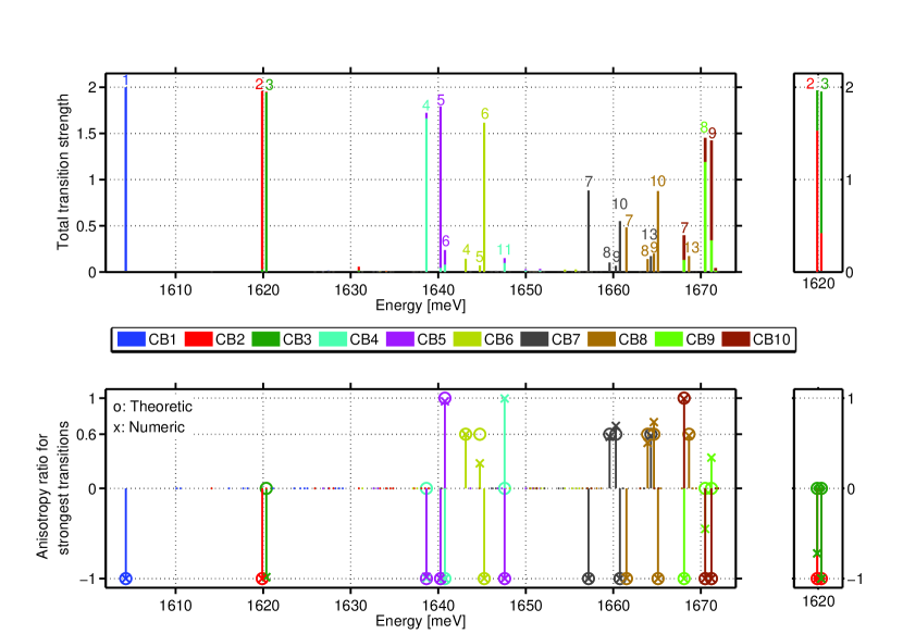
Figure 19: The top subplot show the combined optical oscillator strength, $\bar{M}_{x}+\bar{M}_{y}+\bar{M}_{z}$, as a function of energy. The colors label the contributions due to the individual conduction band levels, and the valence band state number is indicated by numbers. The lower subplot show the anisotropy ratios, $A_{zx}$, for the significant transitions (limit set to $\bar{M}_{x}+\bar{M}_{y}+\bar{M}_{z}$=0.05). The theoretical anisotropy ratio predictions are also included. Some of the anisotropy ratios cannot be predetermined, for these transition the theoretical value has been set to the dummy value 0 to mark them. The inset at the right show the $CBi-VBj,i,j=2,3$ in the C${}_{\textrm{3v}}$ basis.

VII.2 Dominant and missing optical transitions

A first striking feature of the upper part of Fig. 19 is the dominant diagonal character of the optical transitions, i.e. $CBi-VBj$ is most intense for $i=j$. Note that within degenerate CB levels the numbering has been explicitly chosen to respect $CBi-VBj$ diagonality to ease the analysis. This diagonal character is nearly perfect for the ground state transition, as well as for the first pair $i=2,3$, but progressively weakens as one climbs the excitation ladder.

We also clearly see in Fig. 19 that the highest pairs give rise to a richer structure with side peaks due to the valence-band complexity, but still the $(CB7,CB8)$ pair is dominantly diagonally coupled to the $(VB7,VB10)$ pair, and $(CB9,CB10)$ to $(VB8,VB9)$ pair (see Tab. 5). Clearly, cross-coupling like CB7-VB10, e.t.c. also appear as sub-structures within these dominant pairs.

Looking back to the character of the corresponding states in Tabs. 5 and 6, we find that symmetry elevation to D${}_{\textrm{6h}}$ is an important ingredient to explain missing non-diagonal transitions in Fig. 19. However, not all of them are explained. Take for example the set of transitions from the ground conduction band level $CB1-VBj$. Only $CB1-VB1$ is observed. In principle, using double group selection rules in C${}_{\textrm{3v}}$, all values of $j$ are permitted from $CB1$ in $x-y$-polarization, but in D${}_{\textrm{6h}}$ only $j=1,5,6,11,12,14$ are permitted. In $z$-polarization $j=2-5,8,9,11-13,15$ are permitted in C${}_{\textrm{3v}}$ whilst only $j=5,11,12$ would be in D${}_{\textrm{6h}}$. Thus symmetry elevation accounts for part of the missing transitions, but obviously it is not enough to explain all of them.

Actually one should consider in addition both the symmetry of the dominant UREF and the presence of the approximate azimuthal and radial quantum numbers to explain all missing transitions for the lowest energy states. This is particularly clear with the set $CB1-VBj$. First, on the basis of the symmetry of the dominant UREF $A_{1,g}$ of $CB1$ and the contributing UREFs of $VBj$, all $z$-polarized lines are forbidden, and only $j=1,6,14$ are allowed in $x-y$ polarization. Second, to explain the remaining missing lines from $CB1$, corresponding to $j=6,14$, it suffices to invoke the approximate selection rule based on the radial quantum number of the dominant UREF, which is $n_{r}=1$ for $CB1$, and $n_{r}=2,3$ for $VB6$ and $VB14$ respectively (see Tabs. 5 and 6).

Let us examine more closely the optical coupling between diagonally coupled pairs, considering the UREFs. In $(CB2,CB3)-(VB2,VB3)$, symmetry elevation to D${}_{\textrm{6h}}$ is not sufficient to predict only $CB2-VB2$ and $CB3-VB3$ transitions as observed in Fig. 19. In this respect, it is interesting to see that if one assumes C${}_{\textrm{3v}}$ symmetry, both the crossed transitions between the pairs ($CB2-VB3$ and $CB3-VB2$) should appear, and indeed this is what we observe in the calculated spectrum in the C${}_{\textrm{3v}}$-symmetrized basis (see side of Fig. 19). The observation of $CB3-VB2$ would witness the D${}_{\textrm{6h}}$-symmetry breaking present in the [111] Luttinger Hamiltonian, and might well be resolvable experimentally, whilst CB2-VB3 would be compatible with both symmetries.

In the higher diagonally coupled pairs $(CB4,CB5)-(VB4,VB5)$ and $(CB9,CB10)-(VB8,VB9)$ the same effects are observed and the same considerations apply. For these two sets of transitions we also see in Fig. 19 the appearance of additional non-diagonal transitions with other levels, a trend which naturally increases with transition energy. The last diagonally coupled pairs $(CB7,CB8)-(VB7,VB10)$ are particularly interesting because the two electronic levels $CB7$ and $CB8$ are non-degenerate, hence in Fig. 19 one observes four dominant peaks for these transitions.

VII.3 Optical anisotropy of dominant transitions

The optical anisotropies are also of fundamental interest. By contrast to the selection rules discussed in the previous section, nearly all optical anisotropies can be explained in C${}_{\textrm{3v}}$ symmetry.

Table 7, with the help of the classification of Tabs. 5 and 6, predicts the anisotropy ratio to be $-1$ for transitions between isolated levels $CBi-VBi,\,i=1\textrm{ or }6$, in agreement with the lower part of Fig. 19.

The transitions between the coupled pairs $(CB7,CB8)$ and $(VB7,VB10)$ are also predicted to have anisotropy ratio $-1$, as is well verified in Fig. 19. However the situation for the other diagonally coupled pairs is more subtle.

In $(CB2,CB3)-(VB2,VB3)$, the optical anisotropy is predicted to be undetermined for the two transitions stemming from $CB3$, and $-1$ for the two stemming from $CB2$. This is satisfied in the C${}_{\textrm{3v}}$-symmetrized basis (see side of Fig. 19), but the anisotropy of both, particularly $CB3-VB3$, is still close to $-1$. The explanation is very simple if one recalls that the LH weight in $VB2$ and $VB3$ is less than 4% (from Tab. 7, the undetermined anisotropy ratios will be close to -1 if the overlap with $\Phi^{E}_{v}$ vanishes). The departure from $-1$ is much bigger for $CB3-VB2$, which can be understood by recalling that this transition should be forbidden in the $x-y$ polarization in D${}_{\textrm{6h}}$ , hence it is more sensitive to LH admixture. We should point out that the disappearance of the transition $CB2-VB3$ in the D${}_{\textrm{6h}}$-symmetrized basis, evidenced in Fig. 19, cannot be understood on the basis of D${}_{\textrm{6h}}$ symmetry alone. We suspect that a study generalizing the magic ratios to D${}_{\textrm{6h}}$ symmetry, linked with the neglect of conduction band spin-splitting, might explain this observation, but the analytical verification would be quite overwhelming.

The optical anisotropy of $(CB4,CB5)-(VB4,VB5)$ and $(CB9,CB10)-(VB8,VB9)$ is entirely similar to $(CB2,CB3)-(VB2,VB3)$ but with the role of the two conduction and valence band levels reversed. We also see that the undetermined anisotropy ratio in transitions from $CB9$ to $(VB8,VB9)$ depart more significantly from any specific values, as is expected due to increased band mixing.

VII.4 Fine structure due to valence-band mixing

Besides the series of dominant peaks there is a fine structure produced by valence band mixing which is particularly interesting to investigate. Fig. 19 shows that such band mixing really starts to be significant from the set of optical transitions $CBi-VBj$ with $i,j\geq 4$.

From the pair $(CB4,CB5)$, weak additional transitions to $VB6$ and $VB11$ are visible in Fig. 19. From the Wigner-Eckart theorem, the transitions to $VB6$ are both allowed in elevated symmetry D${}_{\textrm{6h}}$ whilst towards $VB11$ only $CB5-VB11$ is allowed. We conclude that $CB4-VB11$ is a manifestation of the true C${}_{\textrm{3v}}$ dot symmetry. These weak transitions are slightly more intense in $z$-direction. The anisotropy ratios for the transitions $CB4-VB6$ and $CB5-VB11$ are -1, and for $CB5-VB6$ it is +1, in agreement with C${}_{\textrm{3v}}$ symmetry (Tab. 7). For the remaining $CB4-VB11$ transition the undetermined anisotropy ratio proves to be numerically close to $+1$. Clearly, looking at the corresponding $E_{2,g}$ UREFs, in the spinors Eqs. C.1c and C.1d we may confirm that both +1 transitions are purely due to valence band mixing since only the $E_{1/2,g}$ HSBF (LH-components) can couple to $CB5$.

Besides the next dominant transition $CB6-VB6$, we can see two weak transitions $CB6-VB4$ and $CB6-VB5$ in Fig. 19. Again, both transitions are due to valence band mixing, and are not predicted in elevated symmetry D${}_{\textrm{6h}}$; they manifest the true C${}_{\textrm{3v}}$ symmetry of the QD. The novelty here is that both transitions should have the "magic" anisotropy ratio $3/5$ predicted by Tab. 7. This is very well satisfied by $CB6-VB4$, but $CB6-VB5$ displays a numerical anisotropy ratio close to $0.3$ which will represent the largest deviation from the predicted value in our numerical data. Since its oscillator strength is already rather weak we can safely attribute this deviation to imperfect C${}_{\textrm{3v}}$ symmetrization.

Let us now investigate the weak transitions from the $(CB7,CB8)$ pair to levels $VBj,\,j=8,9,13$. Again these six transitions due to valence band mixing manifest the true C${}_{\textrm{3v}}$ symmetry of the QD, and display quite accurately the “magic” anisotropy ratio $3/5$ for $E_{1/2}(A_{1})-E_{1/2}$ transitions.

The last weak transitions are related to the highest excited pair $(CB9,CB10)$ towards $VB7$ and display polarization anisotropy ratios of $(+1,-1)$ respectively. The symmetry considerations are the same as for $(CB4,CB5)$ to $VB6$ (but correspond to a higher radial excitation), so they are both allowed in D${}_{\textrm{6h}}$ symmetry, and $CB9-VB7$ is a LH transition purely due to valence band mixing.

VII.5 Summary of optical transition spectrum

Optical transitions with polarization perpendicular to the nanowire axis are clearly more dominant for the lowest energy states. This is expected due to the oblate (quantum-well-like) aspect ratio of the QD (Fig. 1), the other optical transitions seen with optical activity polarized along the nanowire axis are linked with valence band mixing and overlap between the conduction band and the LH components. Accordingly, we see an increasing number of transitions with this polarization for higher levels, as the valence band states become increasingly LH-like (see Tab. 5). A computation with more energy levels, or a narrower QD with stronger lateral confinement, would have allowed to reach the ground LH-like level with strong dominance of $z-$polarized optical transitions. Our approach would then evidence the second kind of DPGPS. If the QD aspect ratio would be reversed to prolate a reversal of the roles of HH and LH is expected.

Excitonic effects, which we have neglected in the present work, are not expected to change very much this global picture of polarization anisotropy. It would introduce electron-hole exchange effects which would split all the dominant transitions into a further observable fine structure (which can be seen as quadruplets due to spin degeneracy). The symmetries of the fine-structure excitons can be easily obtained by the product of irreps Dupertuis et al. (2011). Sometimes doublets may remain, other times all lines would split in D${}_{\textrm{6h}}$.

In a real situation, note that the dielectric mismatch between the high index nanowire and the surroundings may filter emission along the nanowire axis, altering the intrinsic optical response of the nanowire QD discussed here.

VIII Conclusion

We have presented a systematic procedure based on class operators for symmetry analysis of the electronic states of a QD. The procedure, called PTCO, is based on postprocessing and alleviates the need for a code specialized with respect to a given symmetry (which would however feature significant gains in memory/time Gallinet et al. ). PTCO has been demonstrated using the $k\cdot{p}$ method for the conduction and valence band of hexagonal GaAs QD grown within Al_0.3Ga_0.7As nanowires. The high D${}_{\textrm{6h}}$ symmetry of the QD heterostructure is partly broken by the C${}_{\textrm{3v}}$ crystal symmetry carried by the Luttinger Hamiltonian, and by the unsymmetric computing grid. Using the PTCO on the computed results, we have been able to sort all these symmetry breaking effects, and quantify them. We have demonstrated that the numerical grid effect was small and could be compensated by PTCO, whilst the deviations from the approximate elevated D${}_{\textrm{6h}}$ symmetry towards the true C${}_{\textrm{3v}}$ symmetry, albeit small, could be measurable.

The PTCO is simple to program, intrinsically systematic and automatized, and is carried out in a single step for a given symmetry, delivering at the same time symmetrized states with corrected energies and a classification for all quantum states. It is flexible, applies independently of the method used to compute the electronic structure, and can be tuned with very little efforts to analyze a higher symmetry in a second run. This enabled us to investigate the proximity of each state to an approximate elevated symmetry.

In a second step, all the quantum states were analyzed using projection operators to give quantitative weights for every symmetry group, for every ultimately reduced envelope function present in every spinorial component. We could then verify all analytical predictions made concerning the UREFs in the elevated D${}_{\textrm{6h}}$ symmetry (App. C). This approach allowed to identify dominant DPGPS and dominant UREFs for all states considered.

The analysis of the dominant UREFs opened the possibility to attribute additional azimuthal and radial quantum numbers to every state. The natural sequence allowed to explain the order of irreps in the computed results, by subduction from $O(3)$ to D${}_{\textrm{6h}}$.

A final summary of the classification is given for all valence band states in Tab. 5, and for all conduction band states in Tab. 6. The classification provides insights into the origin of degeneracies and quasi degeneracies, and allows to predict all selection rules and most of the polarization properties. The information can also be used to construct approximate product states, relevant for the interpretation of excitonic and multi-excitonic fine structure Dupertuis et al. (2011).

Finally we were able to interpret completely all the details of the computed optical spectrum with the help of the classification of the states. We unveiled a large number of missing transitions, which were shown to stem not only from approximate elevated symmetry but also from approximate azimuthal and radial quantum numbers. As valence band mixing was included in the model, we could identify all the corresponding fine structure, responsible for some spread in the optical transition spectrum, and to verify analytical predictions concerning the appearance of "magic ratios" in polarization anisotropy.

High symmetry GaAs nanowire QDs as investigated here are particularly interesting. First, since there are a large number of forbidden transitions in their optical spectrum, the multi-excitonic spectrum is also simplified and can be better interpreted. Second, the doubly degenerate exciton states due to symmetry are well suited for the generation of entangled photons.

Appendix A Choice of standard irreducible matrix representations for C${}_{\textrm{3v}}$ and D${}_{\textrm{6h}}$

For one dimensional irreps $\Gamma$, the set of matrices $\{D^{\Gamma}(g),g\in\mathcal{G}\}$ are simply the characters of the respective irreps i.e. $D^{\Gamma}(g),\chi^{\Gamma}{g},\forall g$, where $\chi^{\Gamma}(g)$ is listed in 26. When $\Gamma$ is of higher dimension, the matrices $\{D^{\Gamma}(g)$ are only unique up to a similarity transform $U(\Gamma)$, i.e.

$$D^{\Gamma}(g)=U(\Gamma)^{-1}\left[D_{\textrm{Alt}}^{\Gamma}(g)\right]^{H}U(\Gamma)$$ (A.1)

where $D_{\textrm{Alt}}^{\Gamma}(g)$ is a matrix irrep listed in 26,and $U(\Gamma)$ is restricted to be unitary. For our purpose the $\left[D_{\textrm{Alt}}^{\Gamma}(g)\right]^{H}$ are not the most numerically convenient since they diagonalize rotations instead of a mirror operation w.r.t. a symmetry plane, e.g. $\sigma_{v1}$ (Fig. 2). We thus choose the following to define our $D^{\Gamma}(g)$ matrices:
C${}_{\textrm{3v}}$, irrep $E$:

$$U_{\textrm{C${}_{\textrm{3v}}$}}(E)=\left[\begin{array}[]{cc}\frac{i}{\sqrt{2}}&\frac{1}{\sqrt{2}}\\ -\frac{i}{\sqrt{2}}&\frac{1}{\sqrt{2}}\end{array}\right]$$ (A.4)

C${}_{\textrm{3v}}$, irrep $E_{1/2}$ (with case A in Ref. 26):

$$U_{\textrm{C${}_{\textrm{3v}}$}}(E_{1/2})=\left[\begin{array}[]{cc}\frac{i}{\sqrt{2}}&\frac{-1}{\sqrt{2}}\\ \frac{1}{\sqrt{2}}&\frac{-i}{\sqrt{2}}\end{array}\right]$$ (A.7)

D${}_{\textrm{6h}}$, irreps $E_{i}$:

$$U_{\textrm{D${}_{\textrm{6h}}$}}(E_{i})=U_{\textrm{C${}_{\textrm{3v}}$}}(E),\,\,i=1..2$$ (A.8)

D${}_{\textrm{6h}}$, irreps $E_{j,k}$:

$$U_{\textrm{D${}_{\textrm{6h}}$}}(E_{j,k})=U_{\textrm{C${}_{\textrm{3v}}$}}(E_{1/2}),\,\,j=\frac{1}{2},\frac{5}{2},k=u,g$$ (A.9)

$$U_{\textrm{D${}_{\textrm{6h}}$}}(E_{3/2,k})=\left[\begin{array}[]{cc}\frac{i}{\sqrt{2}}&\frac{1}{\sqrt{2}}\\ \frac{-1}{\sqrt{2}}&\frac{-i}{\sqrt{2}}\end{array}\right],\,\,k=u,g$$ (A.12)

Note first that our matrix representation obey transposed multiplication tables w.r.t. Ref. 26 (c.f. Hermitian conjugation in Eq. A.1, this is required by our use of the passive rather than the active point of view). Second, our special choice Eq. A.12 for $E_{3/2}$ in D${}_{\textrm{6h}}$ stems from separate requirements concerning the "optimal" choice of HSBF. We ensured in particular that the resulting $E_{3/2,g}$ valence band HSBF was simultaneously the same for D${}_{\textrm{6h}}$ and C${}_{\textrm{3v}}$ symmetry.

Appendix B HSBF for the conduction and valence band spinord in elevated D${}_{\textrm{6h}}$ symmetry

Symmetrized bases Altmann and Herzig (1994), also called Symmetry Adapted Functions (SAF), follow from subduction from $O(3)$ to D${}_{\textrm{6h}}$ and allow to find easily the proper HSBF basis corresponding to the top (bottom) of the valence (conduction) band, respectively, of diamond or Zinc Blende. Unfortunately the SAF in Ref. 26 do not have regular properties under time-reversal, so some care is required.

Let us first consider the bottom of the conduction band, and use linear combinations of zone center Bloch function denoted $\left|{\frac{1}{2},m}\right>^{\bullet}$, $m=\pm\frac{1}{2}$, corresponding to a "quantized axis" with $z$ along [111] and $x$ along $[11\bar{2}]$ Fig. 2. They are nearly odd under spatial inversion in GaAs (hence the $\left|{\dots}\right>^{\bullet}$ symbol as in Ref. 26). Subduction from $O(3)$ tells us that the irrep $E_{1/2,u}$ of D${}_{\textrm{6h}}$ must be associated with this subspace. To construct the HSBF we can either use the SAF of Ref. 26 which are suitable in this case, and the change of basis corresponding to Eq. A.9, or equivalently decide to diagonalize the set of Wigner matrices corresponding to the symmetry operations (parametrization and factor system of Ref. 26), and find their reduction to the set $D^{E_{1/2,u}}(g)$ given in App. A. The resulting conduction band HSBFs are:

$$\left.\begin{array}[]{l}\left|{E_{1/2,u},1}\right>=-\frac{i}{\sqrt{2}}\left|{\frac{1}{2},\frac{1}{2}}\right>^{\bullet}-\frac{1}{\sqrt{2}}\left|{\frac{1}{2},-\frac{1}{2}}\right>^{\bullet}\\ \left|{E_{1/2,u},2}\right>=\frac{1}{\sqrt{2}}\left|{\frac{1}{2},\frac{1}{2}}\right>^{\bullet}+\frac{i}{\sqrt{2}}\left|{\frac{1}{2},-\frac{1}{2}}\right>^{\bullet}\end{array}\right\}$$ (B.3)

For the top of the valence band we use the set of similar Bloch-functions labeled $\left|{\frac{3}{2},m}\right>,\,m=-\frac{3}{2}...\frac{3}{2}$, nearly even under inversion. Then the $O(3)$ subduction tables to D${}_{\textrm{6h}}$ indicate reduction to the $E_{3/2,g}+E_{1/2,g}$ irreps. This time one cannot use all the SAFs of Ref. 26 if one wants to keep an invariant form of the time reversal operator in the HSBF, therefore we follow the route of reducing the Wigner matrices corresponding to symmetry operations. Using a suitable, but freely chosen, set of phase factors compatible with the irreps of App. A, one finds the following D${}_{\textrm{6h}}$ valence band HSBFs:

$$\left.\begin{array}[]{c}\left|{E_{3/2,g},1}\right>=\frac{i}{\sqrt{2}}\left|{\frac{3}{2},\frac{3}{2}}\right>-\frac{1}{\sqrt{2}}\left|{\frac{3}{2},-\frac{3}{2}}\right>\\ \left|{E_{3/2,g},2}\right>=\frac{1}{\sqrt{2}}\left|{\frac{3}{2},\frac{3}{2}}\right>-\frac{i}{\sqrt{2}}\left|{\frac{3}{2},-\frac{3}{2}}\right>\end{array}\right\}$$ (B.4)

and

$$\left.\begin{array}[]{c}\left|{E_{1/2,g},1}\right>=\frac{1}{\sqrt{2}}\left|{\frac{3}{2},\frac{1}{2}}\right>+\frac{i}{\sqrt{2}}\left|{\frac{3}{2},-\frac{1}{2}}\right>\\ \left|{E_{1/2,g},2}\right>=\frac{i}{\sqrt{2}}\left|{\frac{3}{2},\frac{1}{2}}\right>+\frac{1}{\sqrt{2}}\left|{\frac{3}{2},-\frac{1}{2}}\right>\end{array}\right\}$$ (B.5)

This choice satisfies three desirable constraints: 1) the matrix form of the time reversal operator is invariant when the valence band basis is ordered as

$$\{\left|{E_{3/2,g},1}\right>,\left|{E_{1/2,g},1}\right>,\left|{E_{1/2,g},2}\right>,\left|{E_{3/2,g},2}\right>\}$$ (B.6)

hence it preserves the canonical $p,q,r,s$ form (Eq. II.3) of the Luttinger Hamiltonian in this basis, 2) it is also simultaneously a HSBF for C${}_{\textrm{3v}}$, 3) their transformation laws are given by our set of standard representations listed in App. A.

For C${}_{\textrm{3v}}$ the choice Eqs. B.5 and B.4 is in agreement with Ref. 24 with the correspondence

$$\left|{E_{3/2,g},i}\right>\to\left|{{}^{i}E_{3/2}}\right>,\,i=1..2$$ (B.7)

whilst it differs from Ref. 1 by

$$\left.\begin{array}[]{l}\left|{E_{3/2,g},i}\right>\to(-1)^{i}\left|{{}^{3-i}E_{3/2}}\right>\\ \left|{E_{1/2,g},i}\right>\to(-1)^{i}\left|{E_{1/2},3-i}\right>\end{array}\right\},\,i=1..2.$$ (B.8)

Although the matrix representation for C${}_{\textrm{3v}}$ in App. A are the same as in Ref. 1, we had chosen an opposite projective factor system for the improper operations in Ref. 1. The present projective factor system is now the same as in Ref. 26.

Appendix C UREF decompositions of the valence band spinors in the elevated D${}_{\textrm{6h}}$ symmetry

Using the HSBF derived in App. B, Eqs. B.5, B.4 and B.6, it is possible to decompose each spinor into UREFs with the help of Eq. (48) of Ref. 1 and the Clebsch-Gordon coefficients linked with the chosen standard matrix representation of App. A, and involving a minimum of arbitrary phase factors. In case of C${}_{\textrm{3v}}$ symmetry one finds that the UREF decomposition of the main text Eqs. (IV.3), which remain identical to Refs. 1; 24. In case of D${}_{\textrm{6h}}$ symmetry, and in the HSBF basis order given by Eq. B.6 below, one obtains the ungerade valence band spinors given by Eq. C.1. The corresponding gerade spinors have similar expressions where $u\to g$. To lighten the notation we have omitted the main spinor index and the HSBF index in the UREFs, but they can be retrieved easily from the main spinor and the position of the UREF (using Eq. B.6). For clarity the $\phi/\Phi$ UREFs are not the same functions in Eqs. (C.1c)-(C.1d) w.r.t. Eqs. (C.1a)-(C.1b), and we have used the capital $\Phi$ to distinguish the $E_{1}$ and $E_{2}$ UREFs in the $E_{1/2,g}$ HSBF components from the $E_{3/2,g}$ HSBF components.

Subduction rules to C${}_{\textrm{3v}}$ (according to the case A in Ref. 26) will clearly reduce the spinors Eq. C.1 to Eq. IV.3. Since $E_{1}$, $E_{2}$ $\to E$ one might wonder why the partner function indices are reversed for $E_{1}$ w.r.t. $E_{2}$ (or $E$ in C${}_{\textrm{3v}}$) in Eq. C.1 (Eq. IV.3 in the main text). The reason is simple and lies in our choice of matrix representations in App. A, where the representative of $\sigma_{v1}$ has a different sign for $E_{1}$, reversing the $\sigma_{v1}$ parity characteristics.

Finally time reversal symmetry will bring further constraints on the UREFs, e.g. via $K\uline{\Psi}_{1}^{E_{1/2,u}}=\uline{\Psi}_{2}^{E_{1/2,u}}$ and $K\uline{\Psi}_{2}^{E_{1/2,u}}=-\uline{\Psi}_{1}^{E_{1/2,u}}$ due to Kramers degeneracy. Properties similar to Eq. IV.7 can then be readily obtained, but are omitted for clarity.

$$\underline{\psi}_{1}^{E_{1/2,u}}=\frac{1}{\sqrt{2}}\left(\begin{array}[]{c}\phi_{1}^{E_{1,u}}-\phi_{2}^{E_{2,u}}\\ \phi^{A_{1,u}}+\Phi_{2}^{E_{1,u}}\\ \phi^{A_{2,u}}+\Phi_{1}^{E_{1,u}}\\ \phi_{2}^{E_{1,u}}-\phi_{1}^{E_{2,u}}\end{array}\right)$$ (C.1a)

$$\underline{\psi}_{2}^{E_{1/2,u}}=\frac{1}{\sqrt{2}}\left(\begin{array}[]{c}\phi_{2}^{E_{1,u}}+\phi_{1}^{E_{2,u}}\\ -\phi^{A_{2,u}}+\Phi_{1}^{E_{1,u}}\\ \phi^{A_{1,u}}-\Phi_{2}^{E_{1,u}}\\ -\phi_{1}^{E_{1,u}}-\phi_{2}^{E_{2,u}}\end{array}\right)$$ (C.1b)

$$\underline{\psi}_{1}^{E_{3/2,u}}=\frac{1}{\sqrt{2}}\left(\begin{array}[]{c}\phi^{A_{1,u}}-\phi^{B_{2,u}}\\ \Phi_{1}^{E_{1,u}}-\Phi_{2}^{E_{2,u}}\\ \Phi_{2}^{E_{1,u}}+\Phi_{1}^{E_{2,u}}\\ \phi^{A_{2,u}}+\phi^{B_{1,u}}\end{array}\right)$$ (C.1c)

$$\underline{\psi}_{2}^{E_{3/2,u}}=\frac{1}{\sqrt{2}}\left(\begin{array}[]{c}-\phi^{A_{2,u}}+\phi^{B_{1,u}}\\ \Phi_{2}^{E_{1,u}}-\Phi_{1}^{E_{2,u}}\\ -\Phi_{1}^{E_{1,u}}-\Phi_{2}^{E_{2,u}}\\ \phi^{A_{1,u}}+\phi^{B_{2,u}}\end{array}\right)$$ (C.1d)

$$\underline{\psi}_{1}^{E_{5/2,u}}=\frac{1}{\sqrt{2}}\left(\begin{array}[]{c}\phi_{2}^{E_{1,u}}-\phi_{1}^{E_{2,u}}\\ \phi^{B_{1,u}}+\Phi_{2}^{E_{2,u}}\\ \phi^{B_{2,u}}+\Phi_{1}^{E_{2,u}}\\ \phi_{1}^{E_{1,u}}-\phi_{2}^{E_{2,u}}\end{array}\right)$$ (C.1e)

$$\underline{\psi}_{1}^{E_{5/2,u}}=\frac{1}{\sqrt{2}}\left(\begin{array}[]{c}-\phi_{1}^{E_{1,u}}-\phi_{2}^{E_{2,u}}\\ -\phi^{B_{2,u}}+\Phi_{1}^{E_{2,u}}\\ \phi^{B_{1,u}}-\Phi_{2}^{E_{2,u}}\\ \phi_{2}^{E_{1,u}}+\phi_{1}^{E_{2,u}}\end{array}\right)$$ (C.1f)

References

- Dalessi and Dupertuis (2010) S. Dalessi and M. A. Dupertuis, Physical Review B - Condensed Matter and Materials Physics 81 (2010), 10.1103/PhysRevB.81.125106.
- Lauhon et al. (2004) L. Lauhon, M. Gudiksen, and C. Lieber, Philosophical Transactions of the Royal Society A: Mathematical, Physical and Engineering Sciences 362, 1247 (2004).
- Tribu et al. (2008) A. Tribu, G. Sallen, T. Aichele, R. André, J.-P. Poizat, C. Bougerol, S. Tatarenko, and K. Kheng, Nano Letters 8, 4326 (2008).
- Borgström et al. (2005) M. Borgström, V. Zwiller, E. Müller, and A. Imamoglu, Nano Letters 5, 1439 (2005).
- Kats et al. (2012) V. Kats, V. Kochereshko, A. Platonov, T. Chizhova, G. Cirlin, A. Bouravleuv, Y. Samsonenko, I. Soshnikov, E. Ubyivovk, J. Bleuse, and H. Mariette, Semiconductor Science and Technology 27 (2012), 10.1088/0268-1242/27/1/015009.
- Choi et al. (2012) K. Choi, M. Arita, S. Kako, and Y. Arakawa, Journal of Crystal Growth , (2012), in press.
- Dorenbos et al. (2010) S. Dorenbos, H. Sasakura, M. Van Kouwen, N. Akopian, S. Adachi, N. Namekata, M. Jo, J. Motohisa, Y. Kobayashi, K. Tomioka, T. Fukui, S. Inoue, H. Kumano, C. Natarajan, R. Hadfield, T. Zijlstra, T. Klapwijk, V. Zwiller, and I. Suemune, Applied Physics Letters 97 (2010).
- Singh and Bester (2009) R. Singh and G. Bester, Phys. Rev. Lett. 103, 063601 (2009).
- Schliwa et al. (2009) A. Schliwa, M. Winkelnkemper, A. Lochmann, E. Stock, and D. Bimberg, Phys. Rev. B 80, 161307 (2009).
- Imamoglu et al. (1999) A. Imamoglu, D. D. Awschalom, G. Burkard, D. P. DiVincenzo, D. Loss, M. Sherwin, and A. Small, Phys. Rev. Lett. 83, 4204 (1999).
- Oberli et al. (2009) D. Y. Oberli, M. Byszewski, B. Chalupar, E. Pelucchi, A. Rudra, and E. Kapon, Phys. Rev. B 80, 165312 (2009).
- Niquet and Mojica (2008) Y.-M. Niquet and D. Mojica, Physical Review B - Condensed Matter and Materials Physics 77 (2008).
- Zhang and Shi (2011) M. Zhang and J.-J. Shi, Superlattices and Microstructures 50, 529 (2011).
- Ravi Kishore et al. (2010) V. Ravi Kishore, B. Partoens, and F. Peeters, Physical Review B - Condensed Matter and Materials Physics 82 (2010), 10.1103/PhysRevB.82.235425.
- Andreev and O’Reilly (2001) A. D. Andreev and E. P. O’Reilly, Applied Physics Letters 79, 521 (2001).
- Vukmirovic et al. (2005) N. Vukmirovic, D. Indjin, V. Jovanovic, Z. Ikonic, and P. Harrison, Physical Review B - Condensed Matter and Materials Physics 72 (2005), 10.1103/PhysRevB.72.075356.
- Tomic (2006) S. Tomic, Phys. Rev. B 73, 125348 (2006).
- Pryor (1998) C. Pryor, Physical Review Letters 80, 3579 (1998).
- Mlinar and Peeters (2007) V. Mlinar and F. Peeters, Applied Physics Letters 91 (2007), 10.1063/1.2753745.
- Tronc et al. (2004) P. Tronc, V. Smirnov, and K. Zhuravlev, Physica Status Solidi (B) Basic Research 241, 2938 (2004).
- Luttinger and Kohn (1955) J. Luttinger and W. Kohn, Physical Review 97, 869 (1955).
- Fishman (1995) G. Fishman, Physical Review B 52, 11132 (1995).
- Tomic and Vukmirovic (2011) S. Tomic and N. Vukmirovic, Journal of Applied Physics 110, 053710 (2011).
- (24) S. Dalessi, F. Michelini, and M. A. Dupertuis, To be published.
- Guo et al. (2011) J. Guo, H. Huang, X. Ren, X. Yan, S. Cai, Y. Huang, Q. Wang, X. Zhang, and W. Wang, Chinese Optics Letters 9 (2011), 10.3788/COL201109.041601.
- Altmann and Herzig (1994) S. Altmann and P. Herzig, Point-Group Theory Tables (Clarendon press Oxford, 1994) in this work we have used a passive point of view throughout. As a consequence, the group multiplication tables of Altmann should be transposed.
- Messiah (1959) A. Messiah, Quantum mechanics, Vol. II (North-Holland publishing company, 1959) in this work we have used a passive point of view throughout. As a consequence, the Euler and Wigner matrices should be transposed.
- Note (1) Note that in spin space a rotation by is equal to inversion, and a rotation of define the identity operation, . The double group therefore has twice the number of elements compared to the single group.
- Hammermesh (1989) M. Hammermesh, “Group theory and its applications to physical problems,” (Dover, 1989).
- Gallinet et al. (2010) B. Gallinet, J. Kupec, B. Witzigmann, and M.-A. Dupertuis, Journal of the Optical Society of America B: Optical Physics 27, 1364 (2010).
- Dupertuis et al. (2011) M. Dupertuis, K. Karlsson, D. Oberli, E. Pelucchi, A. Rudra, P. Holtz, and E. Kapon, Physical Review Letters 107 (2011), 10.1103/PhysRevLett.107.127403.
- Chen (1989) J. Chen, “Group representation theory for physicists,” (World scientific publishing Co. Pte. Ltd., 1989) Chap. 3, 2nd ed., in the present paper, the class operators will be defined in the solution space, but they still enjoy all the properties derived in Chen.
- Vurgaftman et al. (2001) I. Vurgaftman, J. Meyer, and L. Ram-Mohan, Journal of Applied Physics 89, 5815 (2001).
- Yi et al. (2009) W. Yi, V. Narayanamurti, H. Lu, M. Scarpulla, A. Gossard, Y. Huang, J.-H. Ryou, and R. Dupuis, Applied Physics Letters 95 (2009), 10.1063/1.3224914.
- Karlsson et al. (2010) K. F. Karlsson, M. A. Dupertuis, D. Y. Oberli, E. Pelucchi, A. Rudra, P. O. Holtz, and E. Kapon, Phys. Rev. B 81, 161307 (2010).
- Ba Hoang et al. (2010) T. Ba Hoang, A. F. Moses, L. Ahtapodov, H. Zhou, D. L. Dheeraj, A. T. J. van Helvoort, B.-O. Fimland, and H. Weman, Nano Letters 10, 2927 (2010).
- (37) B. Gallinet, M. A. Dupertuis, and F. Reuse, To be published.