Relic gravitational waves in the frame of slow-roll inflation with a power-law potential and the detection

Abstract

We obtained the analytic solutions of relic gravitational waves (RGWs) for the slow-roll inflation with a power-law form potential of the scalar field, $V=\lambda\phi^{n}$. Based on a reasonable range of $n$ constrained by cosmic microwave background (CMB) observations, we give tight constraints of the tensor-to-scalar ratio $r$ and the inflation expansion index $\beta$ for the fixed scalar spectral index $n_{s}$. Even though, the spectrum of RGWs in low frequencies is hardly depends on any parameters, the high frequency parts will be affected by several parameters, such as $n_{s}$, the reheating temperature $T_{\rm{RH}}$ and the index $\beta_{s}$ describing the expansion from the end of inflation to the reheating process. We analyzed in detail all the factors which would affect the spectrum of RGWs in high frequencies including the quantum normalization. We found that the future GW detectors SKA, eLISA, BBO and DECIGO are promising to catch the signals of RGWs. Furthermore, BBO and DECIGO have the potential not only to distinguish the spectra with different parameters but also to examine the validity of the quantum normalization.

PACS number: 04.30.-w, 98.80.Es, 98.80.Cq

I Introduction

The validity of general relativity and quantum mechanics make sure the generation of a stochastic background of relic gravitational waves (RGWs) grishchuk1 ; grishchuk ; grishchuk3 ; starobinsky ; Maggiore ; Giovannini during the early inflationary stage, whose primordial amplitude could be determined by the quantum normalization at the time of the wave modes crossing the horizon during the inflation. Since the interaction of RGWs with other cosmic components is very weak, the evolution of RGWs are mainly determined by the behavior of cosmic expansion including the current acceleration zhang2 ; Zhang4 . Therefore, RGWs could serve as an unique tool to study the very early Universe earlier than the recombination stage when the cosmic microwave background (CMB) radiation was generated. As an interesting source for gravitational wave (GW) detectors, RGWs exist everywhere and anytime unlike GWs radiated by usual astrophysical process. Moreover, RGWs spread a very broad range of frequency, $10^{-18}-10^{10}$ Hz, making themselves become one of the major scientific goals of various GW detectors with different response frequency bands. The current and planed GW detectors contain the ground-based interferometers, such as LIGO ligo1 , Advanced LIGO ligo2 ; advligo , VIRGO virgo ; virgocurve , GEO geo , KAGRA KAGRA and ET Punturo ; Hild aiming at the frequency range $10^{2}-10^{3}$ Hz; the space interferometers, such as the future eLISA/NGO lisa0 ; lisa which is sensitive in the frequency range $10^{-4}-10^{-1}$ Hz, BBO Crowder ; Cutler and DECIGO Kawamura ; Kudoh which both are sensitive in the frequency range $0.1-10$ Hz; and the pulsar timing array, such as PPTA PPTA ; Jenet and the planned SKA Kramer with the frequency window $10^{-9}-10^{-6}$ Hz. Besides, there some potential very-high-frequency GW detectors, such as the waveguide detector cruise , the proposed gaussian maser beam detector around GHz fangyu , and the 100 MHz detector with a pair of 75-cm baseline synchronous recycling interferometers Akutsu . Furthermore, the very low frequency portion of RGWs also contribute to the anisotropies and polarizations of CMB basko , yielding a magnetic type polarization of CMB as a distinguished signal of RGWs. WMAP Peiris ; Spergel ; Hinshaw ; Komatsu , Planck Planck , the ground-based ACTPol Niemack and the proposed CMBpol CMBpol are of this type.

The reheating temperature, $T_{\rm{RH}}$, carries rich information of the early Universe, and relates to the decay rate of the inflation as $T_{\rm{RH}}\propto\sqrt{\Gamma}$ Kolb ; Nakayama . Recently, the temperature of the reheating, $T_{\rm{RH}}$, was evaluated Mielczarek according to the CMB observations by WMAP 7 Komatsu , combining with the slow-roll inflation scenarios. Furthermore, the resultant RGWs was studied in Tong6 . However, these pieces of work underwent the assumption of a fixed form of the potential of the scalar filed driven the slow-roll inflation, $V(\phi)=\frac{1}{2}m^{2}\phi^{2}$. In this paper, we study a more general case of $V(\phi)=\lambda\phi^{n}$ Turner , where $\lambda$ is constant. Moreover, we adopt the limitation $n<2.1$ obtained from the spectrum of CMB martin . For a non-fixed value of $n$, it is hard to evaluate the temperature of the reheating process, $T_{\rm{RH}}$, using the method employed in Mielczarek . Thus, we choose several values of $T_{\rm{RH}}$ lying in the range of $\sim 10^{4}-10^{8}$ GeV, where the lower limit and the upper limit of $T_{\rm{RH}}$ are obtained from the constraints in martin and Bailly , respectively. In the text, one will see that $n$ and $T_{\rm{RH}}$ affect the increases of the scale factor in the early stages of the Universe. Once all the expansion histories of different stages are determined, the evolutions of the RGWs at various phases can be determined subsequently. For the present time, the solutions of RGWs can be obtained, whose different frequency bands correspond to the k-modes re-entered the horizon at different phases. On the other hand, the anisotropies due to the tensor metric perturbations (gravitational waves) can be scaled to those due to the observations of the scalar perturbations by introducing a parameter $r$ called tensor-to-scalar ratio. Under the frame of the slow-roll inflation scenario, $r$ will be constrained in a narrow range due to the constraints from $n$ for a given value of the scalar spectral index $n_{s}$. Similarly, the inflation expansion index $\beta$ will also be constrained in a narrow range. Besides, there is a simple relation between $n$ and the preheating expansion index $\beta_{s}$ describing the expansion behavior of the universe from the end of inflation to the reheating process. As will be shown below, the RGWs in the very high frequencies are sensitively dependent on the parameters $n_{s}$, $\beta_{s}$ and $T_{\rm{RH}}$. Furthermore, the spectra of RGWs also depends on the condition of the quantum normalization. To this end, the spectra of RGWs given by different parameters and different conditions will confront the various current and planed GW detectors. The future detectors BBO and DECIGO are quite promising not only to determine various parameters but also to examine the validity of the quantum normalization.

Throughout this paper, we use the units $c=\hbar=k_{B}=1$. Indices $\lambda$, $\mu$, $\nu$,… run from 0 to 3, and $i$, $j$, $k$,… run from 1 to 3.

II RGWs in the accelerating universe

In a spatially flat universe, the existence of perturbations modifies the Friedmann-Robertson-Walker metric to be

$$ds^{2}=a^{2}(\tau)[-d\tau^{2}+(\delta_{ij}+h_{ij})dx^{i}dx^{j}],$$ (1)

where $a(\tau)$ is the scale factor, $\tau$ is the conformal time, and $h_{ij}$ stands for the perturbations to the homogenous and isotropic spacetime background. In general, there are three kinds of perturbations: scalar perturbation, vectorial perturbation and tensorial perturbation. In this paper we only consider the tensorial perturbation, that is, gravitational waves. In the transverse-traceless (TT) gauge, $h_{ij}$ satisfies: $\frac{\partial h_{ij}}{\partial x^{j}}=0$ and $h^{i}_{\,\,i}=0$, where we used the Einstein summation convention. In the Fourier $k$-modes space, it can be written as

$$h_{ij}(\tau,{\bf x})=\sum_{\sigma}\int\frac{d^{3}k}{(2\pi)^{3/2}}\epsilon^{(\sigma)}_{ij}h_{k}^{(\sigma)}(\tau)e^{i\bf{k}\cdot{x}},$$ (2)

where $\sigma=+,\times$ stands for the two polarization states, the comoving wave number $k$ is related with the wave vector $\mathbf{k}$ by $k=(\delta_{ij}k^{i}k^{j})^{1/2}$, $h_{-k}^{(\sigma)*}(\tau)=h_{k}^{(\sigma)}(\tau)$ ensuring $h_{ij}$ be real, and the polarization tensor $\epsilon^{(\sigma)}_{ij}$ satisfies grishchuk :

$$\epsilon^{(\sigma)}_{ij}\epsilon^{(\sigma^{\prime}){ij}}=2\delta_{\sigma\sigma^{\prime}},\quad\epsilon^{(\sigma)}_{ij}\delta^{ij}=0,\quad\epsilon^{(\sigma)}_{ij}n^{j}=0,\quad\epsilon^{(\sigma)}_{ij}(-\mathbf{k})=\epsilon^{(\sigma)}_{ij}(\mathbf{k}).$$ (3)

In terms of the mode $h^{(\sigma)}_{k}$, the wave equation is

$$h^{(\sigma)}_{k}{{}^{\prime\prime}}(\tau)+2\frac{a^{\prime}(\tau)}{a(\tau)}h^{(\sigma)}_{k}{{}^{\prime}}(\tau)+k^{2}h^{(\sigma)}_{k}(\tau)=0,$$ (4)

where a prime means taking derivative with respect to $\tau$. The two polarizations of $h^{(\sigma)}_{k}(\tau)$ have the same statistical properties and give equal contributions to the unpolarized RGWs background, so the super index $(\sigma)$ can be dropped. The approximate solutions of Eq. (4) are well analyzed in grishchuk ; grishchuk3 ; zhang2 , and are detailed listed in Tong6 given an accelerating universe at present. Furthermore, the analytic solutions were also studied by many authors Zhang4 ; Yuki ; Miao ; Kuroyanagi ; TongZhang . For a power-law form of the scale factor $a(\tau)\propto\tau^{\alpha}$, the analytic solution to Eq.(4) is a linear combination of Bessel and Neumann functions

$$h_{k}(\tau)=\tau^{\frac{1}{2}-\alpha}\big{[}C_{1}J_{\alpha-\frac{1}{2}}(k\tau)+C_{2}N_{\alpha-\frac{1}{2}}(k\tau)\big{]},$$ (5)

where the constants $C_{1}$ and $C_{2}$ for each stage are determined by the continuities of $h_{k}(\tau)$ and $h^{\prime}_{k}(\tau)$ at the joining points $\tau_{1},\tau_{s},\tau_{2}$ and $\tau_{E}$ Zhang4 ; Miao . Therefore, the all the constants in the solutions of RGWs can be completely fixed, once the initial condition is given. In a spatially flat ($k=0$) universe, the scale factor indeed has a power-law form in various stages grishchuk ; Miao ; TongZhang ; Tong6 . It is described by the following successive stages :

The inflationary stage:

$$a(\tau)=l_{0}|\tau|^{1+\beta},\,\,\,\,-\infty<\tau\leq\tau_{1},$$ (6)

where the inflation index $\beta$ is an model parameter describing the expansion history during inflation. The special case of $\beta=-2$ corresponds the exact de Sitter expansion. However, both the model-predicted and the observed results indicate that the value of $\beta$ could differ slightly from $-2$.

The preheating stage :

$$a(\tau)=a_{z}|\tau-\tau_{p}|^{1+\beta_{s}},\,\,\,\,\tau_{1}\leq\tau\leq\tau_{s},$$ (7)

where the parameter $\beta_{s}$ describes the expansion behavior of the preheating stage from the end of inflation to the happening of reheating process followed by the radiation-dominant stage. In some literatures Starobinsky2 ; Tong6 , $\beta_{s}$ is set to be $1$ , however, we take $\beta_{s}$ as a free parameter in the paper.

The radiation-dominant stage :

$$a(\tau)=a_{e}(\tau-\tau_{e}),\,\,\,\,\tau_{s}\leq\tau\leq\tau_{2}.$$ (8)

The matter-dominant stage:

$$a(\tau)=a_{m}(\tau-\tau_{m})^{2},\,\,\,\,\tau_{2}\leq\tau\leq\tau_{E}.$$ (9)

The accelerating stage up to the present time $\tau_{0}$ zhang2 :

$$a(\tau)=l_{H}|\tau-\tau_{a}|^{-\gamma},\,\,\,\,\tau_{E}\leq\tau\leq\tau_{0},$$ (10)

where $\gamma$ is a $\Omega_{\Lambda}$-dependent parameter, and $\Omega_{\Lambda}$ is the energy density contrast. To be specific, we take $\gamma\simeq 1.97$ zhangtong for $\Omega_{\Lambda}=0.73$ Komatsu in this paper. It is convenient to choose the normalization $|\tau_{0}-\tau_{a}|=1$, i.e., the present scale factor $a(\tau_{0})=l_{H}$. From the definition of the Hubble constant, one has $l_{H}=\gamma/H_{0}$, where $H_{0}=100\,h$ km s^-1Mpc^-1 is the present Hubble constant. We take $h\simeq 0.704$ Komatsu throughout this paper. Supposing $\beta$ and $\beta_{s}$ are model parameters, all the constants included trough Eq.(6) to Eq. (10) can be fixed by the continuity of $a(\tau)$ and $a^{\prime}(\tau)$ at the four given joining points $\tau_{1}$, $\tau_{s}$, $\tau_{2}$ and $\tau_{E}$, if one knows the increases of the scale factor of various stages, i.e., the definite values of $\zeta_{1}\equiv{a(\tau_{s})}/{a(\tau_{1})}$, $\zeta_{s}\equiv{a(\tau_{2})}/{a(\tau_{s})}$, $\zeta_{2}\equiv{a(\tau_{E})}/{a(\tau_{2})}$, and $\zeta_{E}\equiv{a(\tau_{0})}/{a(\tau_{E})}$.

The spectrum of RGWs $h(k,\tau)$ is defined by

$$\langle h^{ij}(\tau,\mathbf{x})h_{ij}(\tau,\mathbf{x})\rangle\equiv\int_{0}^{\infty}h^{2}(k,\tau)\frac{dk}{k},$$ (11)

where the angle brackets mean ensemble average. The dimensionless spectrum $h(k,\tau)$ relates to the mode $h_{k}(\tau)$ as TongZhang

$$h(k,\tau)=\frac{\sqrt{2}}{\pi}k^{3/2}|h_{k}(\tau)|.$$ (12)

The one that we are of interest is the present RGWs spectrum $h(k,\tau_{0})$. The characteristic comoving wave number at a certain joining time $\tau_{x}$ is give by Tong6

$$k_{x}\equiv k(\tau_{x})=\frac{2\pi a(\tau_{x})}{1/H(\tau_{x})}.$$ (13)

After a long but simple calculation, it is easily to obtain $k_{H}=2\pi\gamma$ and the following relations:

$$\frac{k_{E}}{k_{H}}=\zeta_{E}^{-\frac{1}{\gamma}},\quad\frac{k_{2}}{k_{E}}=\zeta_{2}^{\frac{1}{2}},\quad\frac{k_{s}}{k_{2}}=\zeta_{s},\quad\frac{k_{1}}{k_{s}}=\zeta_{1}^{\frac{1}{1+\beta_{s}}}.$$ (14)

In the present universe, the physical frequency relates to a comoving wave number $k$ as

$$f=\frac{k}{2\pi a(\tau_{0})}=\frac{k}{2\pi l_{H}}.$$ (15)

The present energy density contrast of RGWs defined by $\Omega_{GW}=\langle\rho_{g}\rangle/{\rho_{c}}$, where $\rho_{g}=\frac{1}{32\pi G}h_{ij,0}h^{ij}_{,0}$ is the energy density of RGWs and $\rho_{c}=3H_{0}^{2}/8\pi G$ is the critical energy density, is given by grishchuk3 ; Maggiore

$$\Omega_{GW}=\int_{f_{low}}^{f_{upper}}\Omega_{g}(f)\frac{df}{f},$$ (16)

with

$$\Omega_{g}(f)=\frac{2\pi^{2}}{3}h^{2}_{c}(f)\Big{(}\frac{f}{H_{0}}\Big{)}^{2}$$ (17)

being the dimensionless energy density spectrum. We have used a new notation, $h_{c}(f)=h(f,\tau_{0})/\sqrt{2}$, called characteristic strain spectrum Maggiore or chirp amplitude Boyle . The lower and upper limit of integration in Eq.(16) can be taken to be $f_{low}\simeq f_{E}$ and $f_{upper}\simeq f_{1}$, respectively, since only the wavelength of the modes inside the horizon contribute to the total energy density.

III The increases of the scale factor

For the simple $\Lambda$CDM model, the late-time acceleration of the universe is well know. One easily has $\zeta_{E}=1+z_{E}=({\Omega_{\Lambda}}/{\Omega_{m}})^{1/3}\simeq 1.4$, where $z_{E}$ is the redshift when the accelerating expansion begins. The increase of the scale factor duration of the matter-dominated stage can also be obtained straightforwardly, $\zeta_{2}=\frac{a(\tau_{0})}{a(\tau_{2})}\frac{a(\tau_{E})}{a(\tau_{0})}=(1+z_{eq})\zeta_{E}^{-1}$ with $z_{eq}=3240$ Komatsu . However, the histories of the radiation-dominated stage and the preheating stage are not known well. Recently, Mielczarek Mielczarek proposed a method to evaluate the reheating temperature, $T_{\rm{RH}}$, under the frame of the slow-roll inflation model with a quadratic potential $V(\phi)=\frac{1}{2}m^{2}\phi^{2}$ combing the observations from WMAP. Using this method, $\zeta_{s}$ and $\zeta_{1}$ can be determined subsequently with the evaluation of $T_{\rm{RH}}$ Tong6 . In this paper, we consider a more general power-law form of the potential, $V(\phi)=\lambda\phi^{n}$, where $\lambda$ is a constant. For this general form of $V(\phi)$, it is hard to obtain the analytic expression of the energy density of the universe at the end of inflation, and in turn, it is hard to obtain the temperature of reheating analytically. Hence, we will take some reasonable values of $T_{\rm{RH}}$ constrained by CMB observationsmartin .

Firstly, we discuss the value of $\zeta_{s}$. After reheating, the universe is filled with the relativistic plasma, which undergoes a adiabatic expansion as long as the entropy transfer between the radiation and other components can be neglected. The adiabatic approximation leads to the conservation of the entropy, i.e., $dS=0$. It implies $sa^{3}=$const, where the entropy density $s$ of radiation is given by

$$s=\frac{2\pi^{2}}{45}g_{s}T^{3}.$$ (18)

Here, $g_{s}$ counts the effective number of relativistic species contributing to the radiation entropy. Another similar quantity $g$, counting the effective number of relativistic species contributing to the energy density of radiation, relates to energy density:

$$\rho=\frac{\pi^{2}}{30}gT^{4}.$$ (19)

The behavior of $g$ and $g_{s}$ with different energy scale were demonstrated in Yuki . At the energy above $\sim 0.1$ MeV, one has $g=g_{s}$. Moreover, at the energy scales above $\sim 1$ TeV, $g=106.75$ in the standard model, and $g\simeq 220$ in the minimal extension of supersymmetric standard model, respectively. On the other hand, at the energy scales below $\sim 0.1$ MeV, $g=3.36$ and $g_{s}=3.91$ respectively. According to the conservation of entropy, one can easily gets the increase of the scale factor from the reheating till the recombination Mielczarek ,

$$\frac{a_{rec}}{a(\tau_{s})}=\frac{T_{\rm{RH}}}{T_{rec}}\left(\frac{g_{\ast s}}{g_{\star s}}\right)^{1/3},$$ (20)

where $a_{rec}$ and $T_{rec}$ stand for the scale factor and the temperature at the recombination, respectively. $g_{\ast s}$ and $g_{\star s}$ count the effective number of relativistic species contributing to the entropy during the reheating and that during recombination, respectively. As discussed in martin , the lower band of the reheating energy scale is $17.3$ TeV constrained by the observed scalar power spectrum of CMB at $95\%$ of the confidence limit. Thus, in this paper we assume $g_{\ast s}\simeq 200$ eclectically, which was also employed in martin . On the other hand, one has $g_{\star s}=3.91$ including the contributions of the effective number from photons and three species of massless neutrinos to the radiation entropy during the recombination, since the energy scale at the recombination $T_{rec}=T_{\rm{CMB}}(1+z_{rec})\sim 10^{-7}$ MeV. Under the assumption of $g_{\ast s}\simeq 200$, the lower bound of $T_{\rm{RH}}\gtrsim 6\cdot 10^{3}$ GeV was obtained martin . On the other hand, gravitinos production gives an upper bound gravitinos . For instance, in the framework of the Constrained minimal supersymmetric standard model Bailly , the upper bound of $T_{\rm{RH}}$ was found that $T_{\rm{RH}}\lesssim$ a few $\times 10^{7}$ GeV from over-production of ${}^{6}\rm{Li}$ from bound state effects, and moreover, $T_{\rm{RH}}$ can be relaxed to $\lesssim$ a few $\times 10^{8}$ GeV when a more conservative bound on ${}^{6}\rm{Li}/^{7}\rm{Li}$ was used. However, if one does not consider the gravitinos production problem, the most upper bound of $T_{\rm{RH}}$ could be up to $\lesssim 3\cdot 10^{15}$ GeV coming from the energy scale at the end of inflation martin . Based on Eq. (20), one easily obtain

$$\zeta_{s}=\frac{a(\tau_{2})}{a_{rec}}\frac{a_{rec}}{a(\tau_{s})}=\frac{T_{\rm{RH}}}{T_{\rm{CMB}}(1+z_{eq})}\left(\frac{g_{\ast s}}{g_{\star s}}\right)^{1/3},$$ (21)

where we have used $T_{rec}=T_{\rm{CMB}}(1+z_{rec})$. With $T_{\rm{CMB}}=2.725\ {\rm{K}}=2.348\cdot 10^{-13}$ GeV Komatsu , one has $\zeta_{s}\simeq 5\times 10^{16}$ for example. Secondly, we discuss the evaluation of $\zeta_{1}$. First of all, we briefly recall the slow-roll inflation model. For slow-roll inflation, the evolution is described by the usual slow-roll parameters LiddleA :

$$\epsilon\equiv\frac{m^{2}_{Pl}}{16\pi}\left(\frac{V^{\prime}}{V}\right)^{2},\qquad\eta\equiv\frac{m^{2}_{Pl}}{8\pi}\frac{V^{\prime\prime}}{V},$$ (22)

which are required to be much small than unity for the slow-roll approximation to be valid. $\epsilon$ approaches to unity at the end of inflation. When the slow-roll conditions are satisfied, inflation continues keeping the Hubble rate nearly constant, and the primordial tensor power spectrum and the scalar power spectrum are respectively given as Boyle ; Kuroyanagi :

$$\Delta_{h}^{2}(k,\tau_{\ast})\approx\frac{16}{\pi}\left(\frac{H_{\ast}}{m_{\rm{Pl}}}\right)^{2},$$ (23)

$$\Delta_{\mathcal{R}}^{2}(k,\tau_{\ast})\approx\frac{1}{\pi\epsilon}\left(\frac{H_{\ast}}{m_{\rm{Pl}}}\right)^{2},$$ (24)

where $H_{\ast}$ is the Hubble rate during inflation, and $\tau_{\ast}$ stands for the moment when the $k$-mode exits the horizon. On the other hand, based on the observations of CMB, the present scalar power spectrum can be expanded in power laws,

$$\Delta_{h}^{2}(k)=\Delta_{h}^{2}(k_{0})\left(\frac{k}{k_{0}}\right)^{n_{t}},$$ (25)

$$\Delta_{\mathcal{R}}^{2}(k)=\Delta_{\mathcal{R}}^{2}(k_{0})\left(\frac{k}{k_{0}}\right)^{n_{s}-1},$$ (26)

where $\Delta^{2}_{h}(k_{0})$ and $\Delta^{2}_{\mathcal{R}}(k_{0})$ are the power spectrum of the tensor perturbations and curvature perturbations evaluated at the pivot wave number $k_{0}^{\rm{p}}=k_{0}/a(\tau_{0})=0.002$ Mpc^-1 Komatsu , respectively. Furthermore, under the slow-roll approximation, at the pivot wave number $k_{0}$ the spectral parameters are given by LiddleA

$$n_{t}\simeq-2\epsilon,$$ (27)

$$n_{s}\simeq 1-6\epsilon+2\eta,$$ (28)

In general, the spectral indices $n_{t}$ and $n_{s}$ are $k-$depedent, described by the running parameters $\alpha_{t}\equiv dn_{t}/d\ln k$ and $\alpha_{s}\equiv dn_{s}/d\ln k$, respectively grishchuk91 ; Kosowsky ; LiddleA ; TongZhang . However, $\alpha_{t}$ and $\alpha_{s}$ are only second order small quantities. Moreover, if one uses the quantum normalization (see below) as the initial condition for the generation of RGWs, $\alpha_{t}$ should be exactly zero. On the other hand, as will be seen below, non-zero $\alpha_{s}$ would induce an $n_{s}$ greater than 1, which make us difficult to evaluate the increase of the scale factor from the $k_{0}$ mode exiting the horizon during inflation to the end of inflation. Hence, in this paper we will simply set $\alpha_{t}=\alpha_{s}=0$. Note that Even though the value of $n_{t}$ is quite uncertain, $n_{s}$ can be well constrained by CMB Komatsu or BAO Sanchez . The ratio of the primordial tensor power spectrum to the scalar power spectrum is defined as Boyle ; Kuroyanagi

$$r\equiv\frac{\Delta_{h}^{2}(k,\tau_{\ast})}{\Delta_{\mathcal{R}}^{2}(k,\tau_{\ast})}=16\epsilon,$$ (29)

based on Eqs.(23) and (24). Therefore, at the pivot number $k_{0}$, one has

$$r=\frac{\Delta_{h}^{2}(k_{0},\tau_{i})}{\Delta_{\mathcal{R}}^{2}(k_{0},\tau_{i})}\simeq\frac{\Delta_{h}^{2}(k_{0})}{\Delta_{\mathcal{R}}^{2}(k_{0})},$$ (30)

where $\tau_{i}$ is the $k_{0}$-mode exit the horizon during inflation. The approximation of the second equation in Eq.(30) accounts for that the pivot $k_{0}$ wave mode reentered the horizon a little earlier than the present time, and then has suffered a decay. Therefore, the ratio ${\Delta_{h}^{2}(k_{0})}/{\Delta_{\mathcal{R}}^{2}(k_{0})}$ can not exactly reflect the true value of $r$ given by its definition, however, the deviation would be expected to be less than $\sim 0.8\%$ Tong6 . Hence, we will use this approximation when confront with the CMB observations. Furthermore, under this approximation, one has a simple relation:

$$n_{t}=2\beta+4,$$ (31)

since the primordial spectrum of RGWs has a power-law form $\Delta(k_{0})\simeq\Delta(k_{0},\tau_{i})\propto k^{2\beta+4}$ Tong6 . WMAP 7 Mean Komatsu fixed $\Delta^{2}_{\mathcal{R}}(k_{0})\equiv A_{s}=(2.43\pm 0.11)\cdot 10^{-9}$. Thus, the non-zero value of $r$ implies the existence of gravitational wave background, which induced uniquely the B-mode polarization of CMB Amarie . At present only observational constraints on $r$ have been given Komatsu ; Hinshaw . The upper bounds of $r$ are recently constrained Komatsu as $r<0.24$ by WMAP+BAO+$H_{0}$ and $r<0.36$ by WMAP 7 only for $\alpha_{s}=0$, and $r<0.49$ for $\alpha_{s}\neq 0$ by both the combination of WMAP+BAO+$H_{0}$ and the WMAP 7 only, respectively. Furthermore, using a discrete, model-independent measure of the degree of fine-tuning required, if $0.95\lesssim n_{s}<0.98$, in accord with current measurements, the tensor-to-ratio satisfies $r\gtrsim 10^{-2}$ Boyle2 . Therefore, one can normalize the RGWs at $k=k_{0}$ using Eq. (30), if $r$ can be determined definitely.

As analyzed by Mielczarek Mielczarek , for the pivot wave number $k_{0}^{\rm{p}}$, the total increase of the scale factor from the mode exit the horizon during inflation up to the present time can be evaluated as

$$\zeta_{\rm{tot}}\simeq\frac{H_{\ast}}{k_{0}^{\rm{p}}}.$$ (32)

Due to Eqs. (24) and (26), one has

$$\frac{1}{\pi\epsilon}\left(\frac{H_{\ast}}{m_{\rm{Pl}}}\right)^{2}\approx\Delta_{\mathcal{R}}^{2}(k_{0}),$$ (33)

where the approximation $\Delta_{\mathcal{R}}^{2}(k_{0})\approx\Delta_{\mathcal{R}}^{2}(k_{0},\tau_{i})$ was used. Taking the form $V(\phi)=\lambda\phi^{n}$, one can easily have a relation:

$$\epsilon=\frac{n(1-n_{s})}{2(n+2)}$$ (34)

from Eqs. (22) and (28). Plugging Eqs. (33) and (34) into Eq. (32) gives

$$\zeta_{\rm{tot}}\simeq\frac{m_{\rm{Pl}}}{k_{0}^{\rm{p}}}\sqrt{\frac{\pi n}{2(n+2)}(1-n_{s})\Delta_{\mathcal{R}}^{2}(k_{0})}.$$ (35)

On the other hand, if we assume the universe did a quasi-de Sitter expansion($\beta\approx-2$), the increase of a scalar factor from the moment of $k_{0}$ mode exiting the horizon during inflation to the end of inflation is give by

$$\zeta_{i}=e^{N},$$ (36)

where $N$ is the e-folding number, which can be estimated as

$$N\simeq-\frac{8\pi}{m^{2}_{\rm{Pl}}}\int_{\phi_{obs}}^{0}\frac{V(\phi)}{V^{\prime}(\phi)}d\phi.$$ (37)

Concretely, for $V(\phi)=\lambda\phi^{n}$, one can get

$$N\simeq\frac{n+2}{2(1-n_{s})},$$ (38)

with the help of Eqs. (22) and (28). So, if $n=2$, Eq.(38) reduces to the result shown in Mielczarek . Plugging Eq. (38) into Eq. (36), and using the identity

$$\zeta_{\rm{tot}}=\zeta_{i}\zeta_{1}\zeta_{s}\zeta_{2}\zeta_{E},$$ (39)

one can easily obtain the complete expression of $\zeta_{1}$:

$$\zeta_{1}=\frac{m_{\rm{Pl}}}{k_{0}^{\rm{p}}}\left[\pi\Delta_{\mathcal{R}}^{2}(k_{0})(1-n_{s})\frac{n}{2(n+2)}\right]^{1/2}\frac{T_{\rm{CMB}}}{T_{\rm{RH}}}\left(\frac{g_{\star s}}{g_{\ast s}}\right)^{1/3}\exp{\left[-\frac{n+2}{2(1-n_{s})}\right]}.$$ (40)

One can examine that, for $n=2$, the above expression reduces to Eq. (11) in Ref.Tong6 after using Eq.(7) in the same reference. In the following, let us see the reasonable range of the index $n$ constrained by both theories and observations. As well known, at the end of inflation, the scalar field $\phi$ oscillates quickly around some point where $V(\phi)$ has a minimum. In the limit that the oscillation rate is much greater than Hubble expansion rate $H$, and ignoring the coupling between the scalar field $\phi$ and other components, it is found that Turner the scalar field oscillations behave like a fluid with $p=\bar{w}\rho$, where the average equation of state $\bar{w}$ depends on the form of the potential $V(\phi)$. For $V(\phi)=\lambda\phi^{n}$, one has

$$\bar{w}=\frac{n-2}{n+2}$$ (41)

and $\rho$ decreases as $a^{-6n/(n+2)}$. In particular, $n=2$, one has $\bar{w}=0$ and $\rho\propto a^{-3}$, which imply a matter-dominant like expansion of the preheating stage Starobinsky2 . Adding the consideration of the coupling between the scalar field and the resulting relativistic particle creation, Martin and Ringeval martin verified the relation (41) using a numerical method, and it was found that the average $\bar{w}$ never deviates from zero exceeding $8\%$. From theoretical consideration, one should have $\bar{w}<1$ to satisfy the positivity energy conditions; while $\bar{w}>-1/3$ to make sure the inflation must stop and the preheating stage begins. Due to Eq. (41), the condition $-1/3<\bar{w}<1$ leads to $n>1$. On the other hand, Martin and Ringeval martin firstly gave a constraint on $n$ based on the CMB observations, $n<2.1$. Therefore, based on both the theories and observations, the index $n$ is constrained to be

$$1<n<2.1.$$ (42)

Note that, there is a relation between $n$ and $\beta_{s}$. According to the energy conservation equation and the Friedmann Equation,

$$\dot{\rho}+3\frac{\dot{a}}{a}\rho(1+\bar{w})=0,$$ (43)

$$\left(\frac{\dot{a}}{a}\right)^{2}=\frac{8\pi G}{3}\rho,$$ (44)

one can easily obtain $a\propto t^{2/(3+3\bar{w})}\propto\tau^{{2}/{(1+3\bar{w})}}$. Using Eqs. (7) and (41), and allowing for $\rho\propto a^{-6n/(n+2)}$, one has

$$\beta_{s}=\frac{4-n}{2(n-1)}.$$ (45)

Then, in principle, the expression of $\zeta_{1}$ in Eq. (40) can be rewritten as a function of $\beta_{s}$. From the combination of Eqs. (42) and (45), one finds that, $n>1$ leads to $\beta_{s}>-0.5$ and $n<2.1$ leads to $\beta_{s}>0.86$, respectively. Based on the range of $n$ (or $\beta_{s}$) discussed above, we try to constrain some parameters combining with CMB observations.

IV Parameters constraints from observations

As shown in the previous section, many parameters are dependent on the value of $n_{s}$. Seven-year WMAP Mean Komatsu gives $n_{s}=0.967\pm 0.014$, and $n_{s}=0.982^{+0.020}_{-0.019}$ when one also considers the tensor mode contributions to the anisotropies of CMB. Moreover, the combination WMAP+BAO+$H_{0}$ Mean gives $n_{s}=0.968\pm 0.012$, and $n_{s}=0.973\pm 0.014$ when the tensor mode contributions are included. Independently, SDSS III predicts $n_{s}=0.96\pm 0.009$ Sanchez . As can be seen in Eq. (40), $\zeta$ is sensitively dependent on $n_{s}$, and in turn one can expect that the spectrum of RGWs also depend sensitively on $n_{s}$ in the very high frequencies. Therefore, for a general demonstration, we consider the cases: $n_{s}=0.96,0.97$ and $0.98$, respectively.

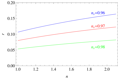
Figure 1: The relation between $r$ and $n$ for the fixe value of $n_{s}=0.96$, $n_{s}=0.97$ and $n_{s}=0.98$, respectively.

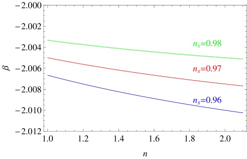
Figure 2: The relation between $\beta$ and $n$ for the fixe value of $n_{s}=0.96$, $n_{s}=0.97$ and $n_{s}=0.98$, respectively.

Firstly, let us constrain the tensor-to-scalar ratio $r$. According to Eqs. (22) and (29), it is straightly to get

$$r=\frac{8n}{n+2}(1-n_{s}).$$ (46)

We show this relation in Fig.1. One can see that $r$ increases slowly with $n$. $r$ lies in (0.11, 0.16), (0.08, 0.12), and (0.05, 0.08) for $n_{s}=0.96$, $n_{s}=0.97$, and $n_{s}=0.98$, respectively. Similarly, from Eqs. (27) and (31), one has

$$\beta=-2-\frac{n}{2(n+2)}(1-n_{s}),$$ (47)

which is shown in Fig.2. The parameter $\beta$ is constrained in the range of $(-2.007,-2.010)$, $(-2.005,-2.008)$, and $(-2.003,-2.005)$ for $n_{s}=0.96$, $n_{s}=0.97$, and $n_{s}=0.98$, respectively. Therefore, the range of $n$ in Eq. (42) leads to very tight constraints on $r$ and $\beta$, which are limited in very narrow ranges with definite value of $n_{s}$.

Now, let us see the increase of the scale factor during preheating stage $\zeta_{1}$, which is expressed in Eq.(40). We plot it in Fig.3 as a function of $n$ with definite values of $T_{\rm{RH}}$. Allowing for the expansion of the universe, one would expect that $\zeta_{1}>1$. As can be seen in Fig.3, the cases of $n_{s}=0.96$ and $0.97$ can make sure well the resultant $\zeta_{1}$ being much larger than 1, however, the case of $n_{s}=0.98$ can not be compatible with the fact $\zeta_{1}>1$ in the whole range of $n$ shown in Eq.(42). If $n_{s}$ is determined well to be as high as $0.98$, it will give very tight constraints on $n$. Concretely, $n\lesssim 1.7$ and $n\lesssim 1.3$ for $T_{\rm{RH}}=10^{4}$ GeV and $T_{\rm{RH}}=10^{8}$ GeV, respectively.

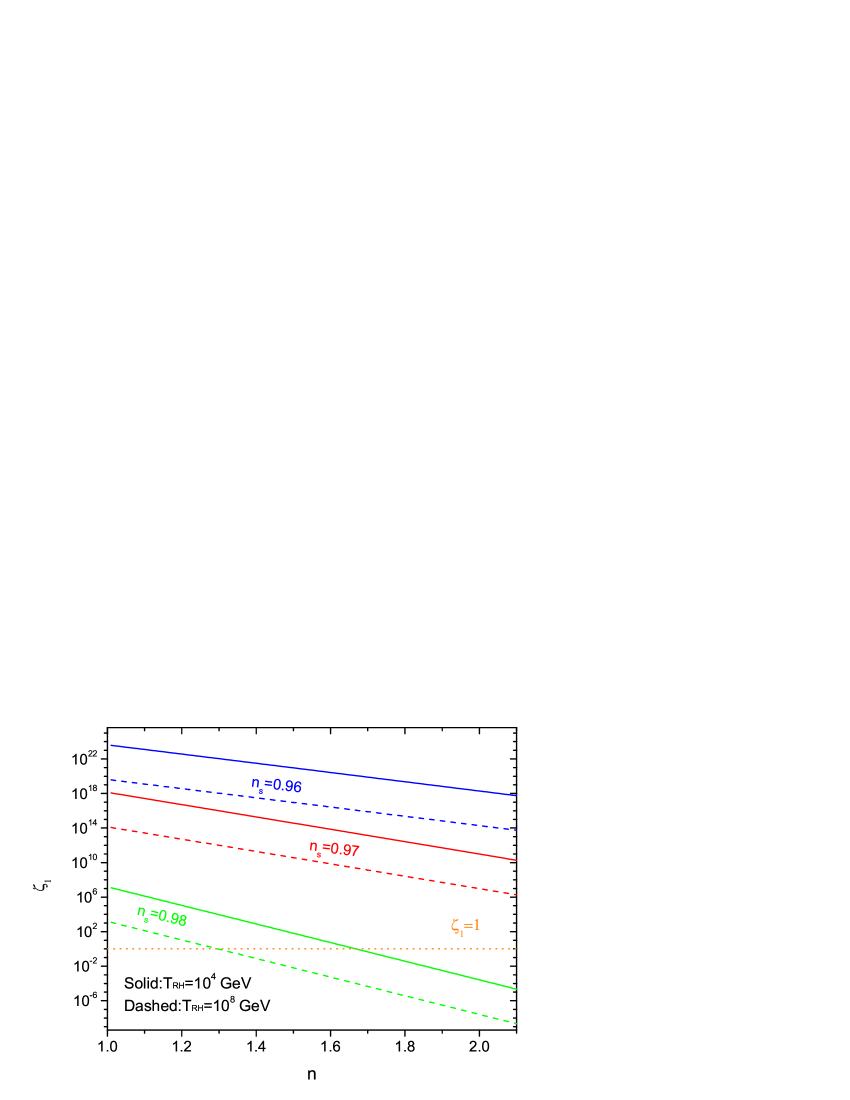
Figure 3: $\zeta_{1}$ as a function of $n$ for the fixed value of $n_{s}=0.96$, $n_{s}=0.97$ and $n_{s}=0.98$, respectively. The solid lines and dashed lines correspond to $T_{\rm{RH}}=10^{4}$ GeV and $T_{\rm{RH}}=10^{8}$ GeV, respectively. The dotted line represents $\zeta_{1}=1$.

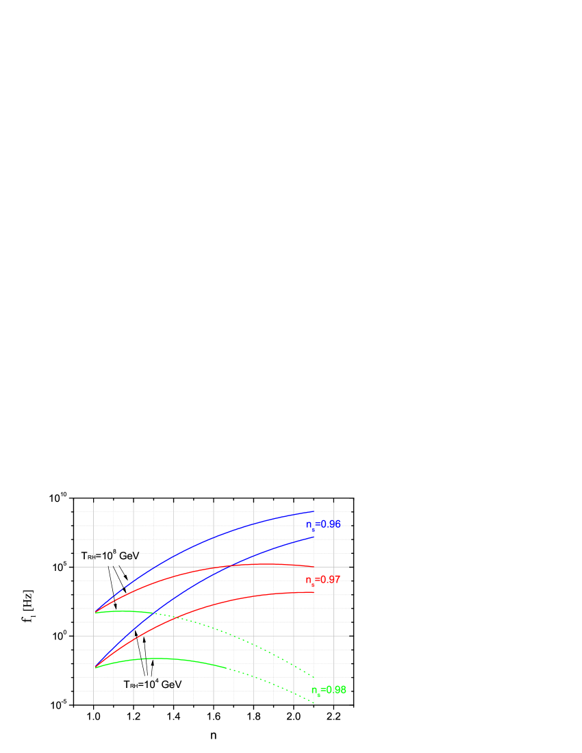
Figure 4: The upper limit frequency $f_{1}$ as a function of $n$ for different combinations of $n_{s}$ and $T_{\rm{RH}}$. The dotted parts for $n_{s}=0.98$ are constrained by the condition $\zeta_{1}>1$ shown in Fig. 3.

What we are more interesting are the characteristic frequencies given by Eq.(15). With the help of Eq. (14), one can easily get the characteristic frequencies: $f_{H}=H_{0}\simeq 2.28\cdot 10^{-18}$ Hz, $f_{H}=H_{0}\simeq 2.28\cdot 10^{-18}$ Hz, $f_{E}\simeq 1.93\cdot 10^{-18}$ Hz, $f_{2}\simeq 9.3\cdot 10^{-17}$ Hz. The value of $f_{s}$ depends linearly on $T_{\rm{RH}}$. For instance, $f_{s}\simeq 4.54\cdot 10^{-3}$ Hz for $T_{\rm{RH}}=10^{4}$ GeV and $f_{s}\simeq 45.4$ Hz for $T_{\rm{RH}}=10^{8}$ GeV, respectively. Since $f_{1}=f_{s}\zeta_{1}^{\frac{1}{1+\beta_{s}}}$, it depends on the values of $n$ (or $\beta_{s}$), $n_{s}$ and $T_{\rm{RH}}$. It is worth to be study in detail, since the characteristic frequency $f_{1}$ is approximately the highest frequency of RGWs. The modes whose frequency higher than $f_{1}$ decay with the expansion of the universe grishchuk ; grishchuk3 . We plot $f_{1}$ as a function of $n$ with definite $n_{s}$ and $T_{\rm{RH}}$ in Fig.4. One can see that the behaviors of $f_{1}$ along with the increasing $n$ are quite different for different values of $n_{s}$. For the case of $n_{s}=0.98$, we plotted $f_{1}$ using dotted lines for the values of $n$ constrained by $\zeta_{1}>1$ which are shown in Fig.3. In the part of large $n$, $f_{1}$ is larger for smaller values of $n_{s}$. On the other hand, in the limit of $n\rightarrow 1$, $f_{1}$ becomes a fixed value independent on $n_{s}$, and moreover, the asymptotic fixed $f_{1}$ is larger for a larger value of $T_{\rm{RH}}$. It is easy to understand if one has found that $\beta_{s}\rightarrow+\infty$ as $n\rightarrow 1$ from Eq.(45) which leads to $f_{1}\rightarrow f_{s}$. The value of $f_{1}$ should be below the constraint from the rate of the primordial nucleosynthesis, $f_{1}\lesssim 3\times 10^{10}$ Hz grishchuk . When the acceleration epoch is considered, the constraint becomes $f_{1}\simeq 4\times 10^{10}$ Hz. This will in turn give some constraints on $n$, $n_{s}$ and $T_{\rm{RH}}$.

As analyzed in our previous work Tong6 , when the quantum normalization for the generation of RGWs during inflation is employed, one has

$$\Delta_{\mathcal{R}}(k_{0})r^{1/2}=8\sqrt{\pi}l_{Pl}H_{0}\zeta_{1}^{\frac{\beta_{s}-\beta}{1+\beta_{s}}}\zeta_{s}^{-\beta}\zeta_{2}^{\frac{1-\beta}{2}}\zeta_{E}^{\frac{\beta-1}{\gamma}}\left(\frac{k_{0}}{k_{H}}\right)^{\beta},$$ (48)

where $l_{Pl}=\sqrt{G}$ is the Planck length. In Eq.(48), there are totally six parameters: $r$, $\beta$, $\beta_{s}$, $n$, $T_{\rm{RH}}$ and $n_{s}$. However, among them only three are independent, due to Eqs.(45), (46) and (47). We show the $T_{\rm{RH}}-\beta$ relation with definite values of $n_{s}$ in Fig.5. First of all, we define the range of $6\cdot 10^{3}-10^{8}$ GeV as Region I; while the range of $6\cdot 10^{3}-3\cdot 10^{15}$ GeV as Region II. It is found that, under the condition of quantum normalization, $n_{s}=0.96$ and $n_{s}=0.98$ can be ruled out, since the resultant $T_{\rm{RH}}$ outside Region II. If one consider the gravitinos production problem, the case $n_{s}=0.97$ would also be ruled out, since the resultant $T_{\rm{RH}}$ outside Region I. However, the resultant $T_{\rm{RH}}$ given by $n_{s}=0.966$ lies well inside Region I for the whole range of $\beta$ given by Eq. (47). Moreover, as shown in Fig.5, the quantum normalization will give a little tighter constraints on the range of $\beta$ for $n_{s}=0.967$ and $n_{s}=0.968$. Note that, these results are based on the validity of quantum normalization, however, it is not the unique initial condition. Let us make a comparison with the previous results in Tong6 . Taking $n_{s}=0.966$ for example, $n=2$ leads to $T_{\rm{RH}}\simeq 3.4\cdot 10^{6}$ GeV; while $T_{\rm{RH}}\simeq 2.8\cdot 10^{12}$ GeV shown in Fig.1 in Ref.Tong6 . Hence, the discrepancy of $T_{\rm{RH}}$, at six orders of magnitude, indicates that the quantum normalization may be not a good initial condition. However, one should also keep in mind that we have used many approximations, which would also contribute a lot to the discrepancy of $T_{\rm{RH}}$ discussed above. Note that, if one does not consider quantum normalization, the zero point energy should be removed or else the cosmological constant would be 120 orders of magnitude larger than observed. Some effective methods Borges have been pointed out. In next section, we will demonstrate the spectra of RGWs with and without quantum normalization respectively.

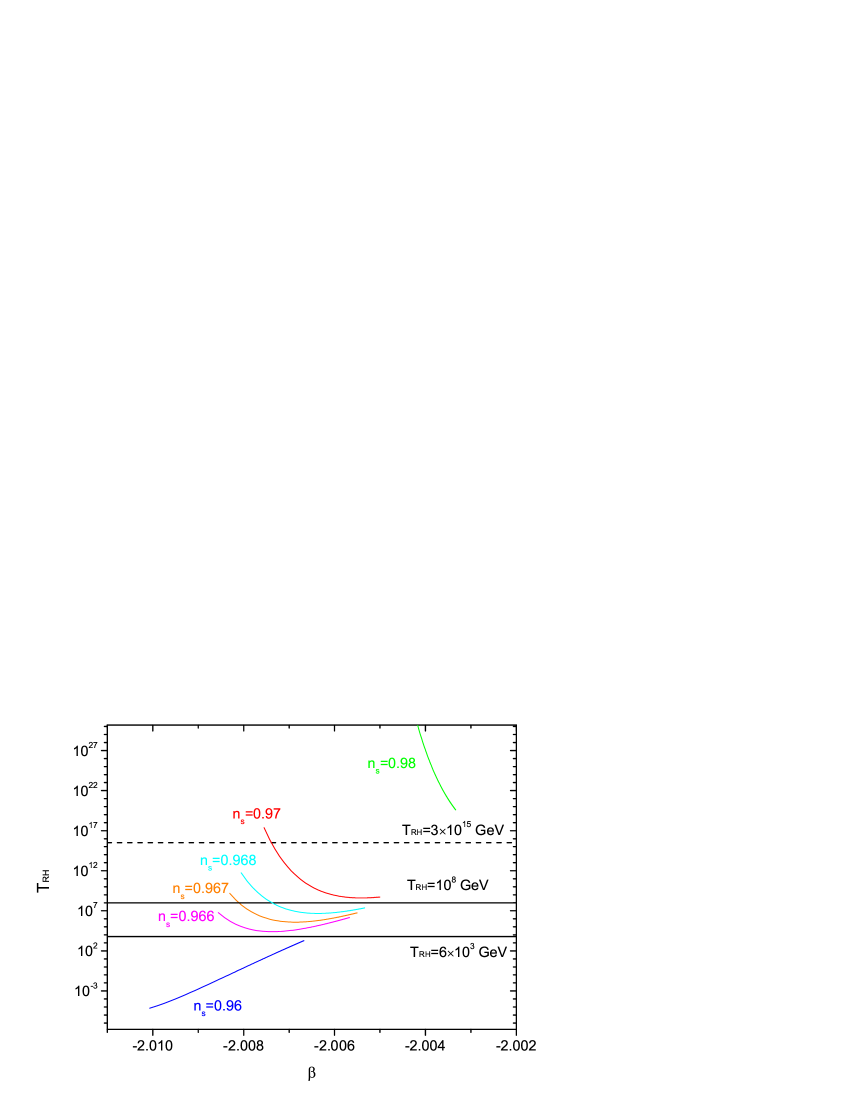
Figure 5: The relation between $T_{\rm{RH}}$ and $\beta$ based on Eq.(48) due to the condition of quantum normalization.

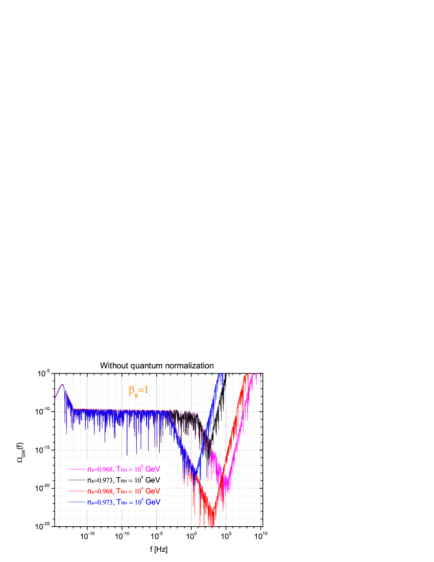
Figure 6: The energy density spectra of RGWs for the fixed $\beta_{s}=1$ with different combinations of $n_{s}$ and $T_{\rm{RH}}$, without considering the quantum normalization.

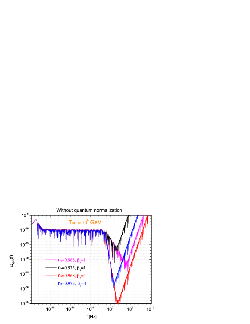
Figure 7: The energy density spectra of RGWs for the fixed $T_{\rm{RH}}=10^{6}$ GeV with different combinations of $n_{s}$ and $\beta_{s}$, without considering the quantum normalization.

V The spectra of RGWs and their detection

In this section, we demonstrate the energy density spectra of RGWs with reasonable values of the parameters and discuss the detection due to the current running and planned gravitational wave detectors.

As discussed in the previous sections, there are many parameters involved in the spectrum of RGWs. They are $n_{s}$, $n$, $r$, $\beta$, $\beta_{s}$, and $T_{\rm{RH}}$. However, among them only three are independent due to Eqs. (45)-(47). Furthermore, $n_{s}$ has been constrained well from observations of CMB, BAO and $H_{0}$. Since the spectrum of RGWs in the high frequencies extreme sensitively depends on $n_{s}$, we discuss two cases of $n_{s}=0.968$ and $n_{s}=0.973$, respectively, based on the combination of WAMP+BAO+$H_{0}$ Komatsu . In the following, we regard $\beta_{s}$ and $T_{\rm{RH}}$ as parameters, and choose some representative values of them since they have large uncertainties. In order to give a complete discussion, we will consider the spectra of RGWS both with and without quantum normalization. As analyzed in Sec.III, $T_{\rm{RH}}$ is constrained to be $T_{\rm{RH}}\sim 10^{4}-10^{8}$ GeV, and $\beta_{s}$ is limited to be larger than $0.86$. Firstly, let us see the case of no quantum normalization. Setting $\beta_{s}=1$, Fig.6 shows the energy density spectra of RGWs, $\Omega_{\rm{GW}}(f)$, with different values of $n_{s}$ and $T_{\rm{RH}}$. One can see that, all the $\Omega_{\rm{GW}}(f)$ nearly overlap each other in the low-frequencies. This is because the spectrum for $f\leq f_{s}$ is only related to $r$ and $\beta$ Tong6 , and, moreover, the differences of $r$ and $\beta$ are very small between the case $n_{s}=0.968$ and the case $n_{s}=0.973$ due to Eqs. (46) and (47). Explicitly, one has $r=0.128,\beta=-2.008$ for $n_{s}=0.968$ and $r=0.108,\beta=-2.007$ for $n_{s}=0.973$, respectively. However, in the part of high frequencies, $\Omega_{\rm{GW}}(f)$ exhibits different properties for different combinations of $n_{s}$ and $T_{\rm{RH}}$. On one hand, for the same value of $T_{\rm{RH}}$, the spectrum $\Omega_{\rm{GW}}(f)$ with $n_{s}=0.968$ and that with $n_{s}=0.973$ have the same “turning point” from which $\Omega_{\rm{GW}}(f)$ decreases rapidly with the increasing frequency, and the “turning point” is just $f_{s}$ which is only dependent on $T_{\rm{RH}}$. Moreover, the decreasing slope of the logarithm of the two spectra for $f\geq f_{s}$ are nearly the same since $\Omega_{\rm{GW}}(f)\propto f^{4+2\beta-2\beta_{s}}$ Tong6 which is reduced to $\Omega_{\rm{GW}}(f)\propto f^{-2}$ for $\beta\approx-2$ and $\beta_{s}=1$. However, the $\Omega_{\rm{GW}}(f)$ with a smaller $n_{s}$ has a larger upper limit frequency $f_{1}$ which responds to a lower amplitude of $\Omega_{\rm{GW}}(f)$. On the other hand, for the same value of $n_{s}$, the $\Omega_{\rm{GW}}(f)$ with a higher $T_{\rm{RH}}$ leads to not only a larger $f_{s}$ but also a larger $f_{1}$ since $f_{1}\propto T_{\rm{RH}}^{1/2}$ for $\beta_{s}=1$ which can seen from the combination of Eqs. (14), (21) and (40). Fig.7 shows the energy density spectra of RGWs for the fixed value $T_{\rm{RH}}=10^{6}$ GeV. One can see that a larger $\beta_{s}$ leads to a steeper slope of the logarithm of $\Omega_{\rm{GW}}(f)$ and a smaller $f_{1}$ for the same values of $n_{s}$. In a word, $T_{\rm{RH}}$ determines the value of $f_{s}$, $\beta_{s}$ determines the slope of the logarithm of $\Omega_{\rm{GW}}(f)$ for the fact that $\beta\approx-2$, and $f_{1}$ depends on all the three parameters especially $n_{s}$. Secondly, let us consider the case of the quantum normalization. Due to the resultant Eq. (48), among the three parameters $T_{\rm{RH}}$, $\beta_{s}$ and $n_{s}$ only two of them are independent. Taking $n_{s}$ and $T_{\rm{RH}}$ as parameters, $\Omega_{\rm{GW}}(f)$ with some combinations of the two parameters are plotted in Fig.8.

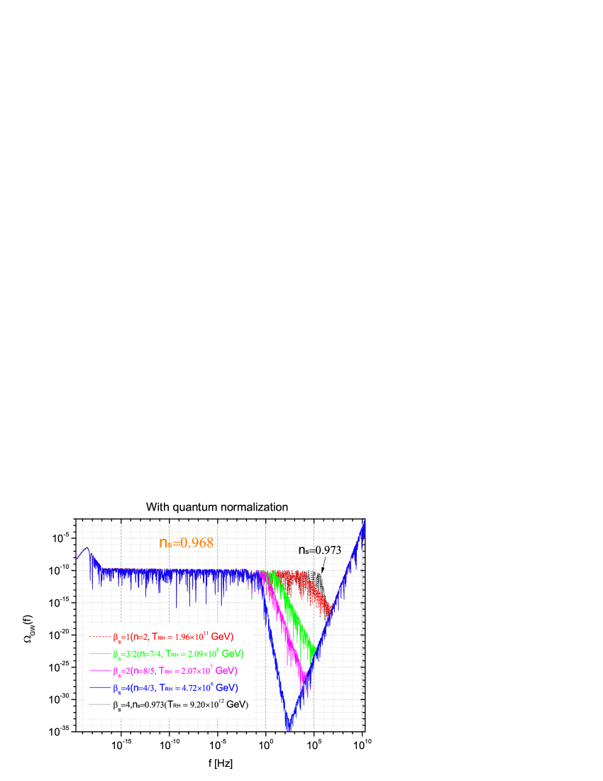
Figure 8: The energy density spectra of RGWs under the condition of the quantum normalization.

Below, let us discuss the detection of RGWs using the ongoing and planned gravitational detectors which are sensitive at different frequency bands. As shown in Fig.6-Fig.8, the differences of the spectra of RGWs with different parameters are only significant in high frequency parts. Hence, we just take a characteristic combination of the parameters $n_{s}=0.968$, $\beta_{s}=1$ and $T_{\rm{RH}}=10^{6}$ GeV for demonstration. As a conservative evaluation, in Fig. 9 we show the strain amplitudes, $h_{c}(f)/\sqrt{f}$ Maggiore of RGWs confronting the strain sensitivity curves of various gravitational wave detectors including the complete PPTA Jenet and SKA Sesana using the pulsar timing technique, and the space-based laser interferometers such as eLISA lisa , BBO Crowder ; Cutler , and the Fabry-Perot DECIGO Kawamura . One can see that, RGWs under the frame of the slow-roll inflation with a potential $V(\phi)\propto\phi^{n}$ are quite promising to be detected by the future SKA, eLISA, BBO and DECIGO. As seen from Fig.6-Fig.8, $\Omega_{\rm{GW}}(f)$ with different parameters have different properties in high frequencies. It would be interesting to discuss the detection of RGWs in high frequencies. In Fig. 10, we plot the characteristic amplitude of RGWs with different parameters and conditions compared to the instrumental noise, $\sqrt{fS_{n}(f)}$, of BBO, the ultimate DECIGO Kudoh , the second generation ground-based laser interferometers AdvLIGO advligo , and the third generation ET Hild . The parameters and conditions of RGWs are listed in Table I. $S_{n}(f)$ is the normal one-side noise spectrum of detectors. As can be seen in Fig.10, even though AdvLIGO and ET are hard to catch the signals of RGWs, BBO has the potential to distinguish RGWs with different parameters or different conditions in the frequency band $10^{-2}-10^{0}$ Hz. Furthermore, the ultimate DECIGO has the capability to distinguish them more easily. Thus, the future BBO and DECIGO detections provide an important tool not only determining the parameters but also examining the validity of the quantum normalization when RGWs were generated during inflation. It is worth to point out that, at frequencies lower than $10^{-2}$ Hz the signals of RGWs are contaminated by the confusion noise produced by galactic binaries Ljz . Hence, we should focus on the frequencies higher than $10^{-2}$ in order to distinguish various spectra of RGWs.

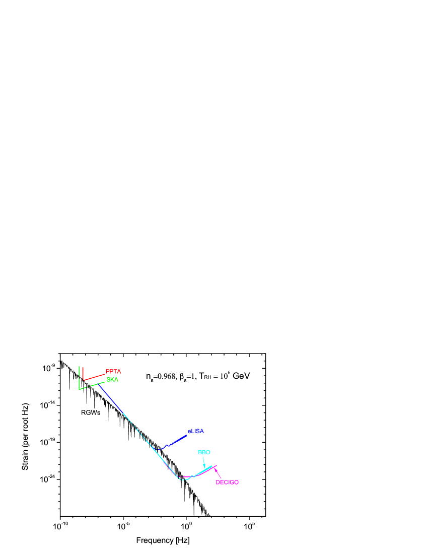
Figure 9: The strain of RGWs with different parameters for $n_{s}=0.968$, $\beta_{s}=1$ and $T_{\rm{RH}}=10^{6}$ GeV confronts against the current and planed GW detectors. The sensitivity curves of PPTA and SKA using pulsar timing technique are taken from Refs.Jenet and Sesana , respectively. The curve of BBO is generated using the online “Sensitivity curve generator” lisa with the parameters in Table II of Ref.Crowder and Table I of Ref.Cutler . The curve of DECIGO is taken from Ref.Kawamura .

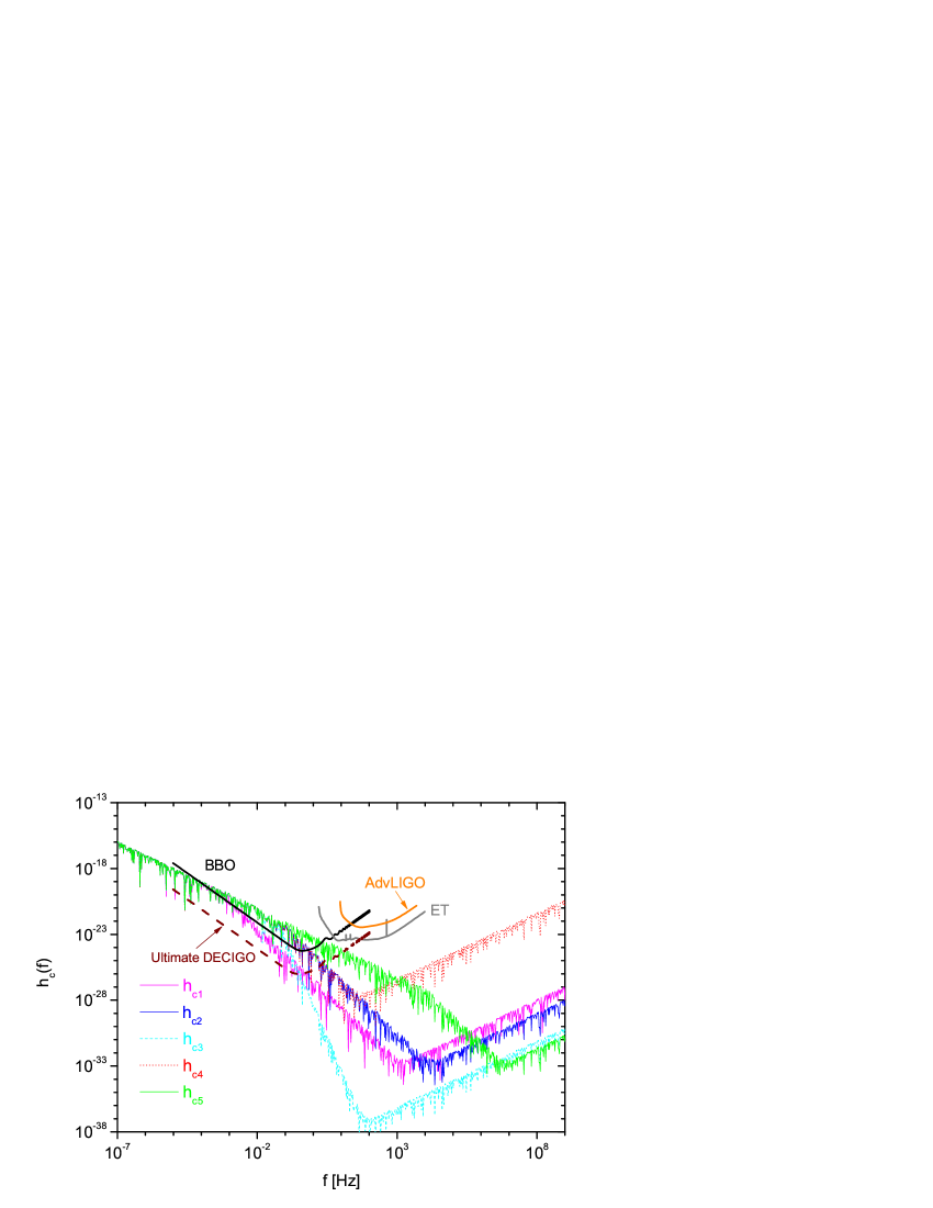
Figure 10: The characteristic amplitude of RGWs in high frequencies confronting against the instrument noise $\sqrt{fS_{n}(f)}$ of BBO, Ultimate DECIGO Kudoh , AdvLIGO and ET.

Table 1: The definitions of $h_{c}$ with different parameters. “N” stands for “No” meaning that the condition of the quantum normalization is not considered; while “Y” stands for “Yes” meaning that the condition of the quantum normalization is considered.

$\quad h_{c}$	$n_{s}$	$\beta_{s}$	$T_{\rm{RH}}$	quantum normalization
$h_{c1}\quad$	$0.968$	$1$	$10^{4}$ GeV	N
$h_{c2}\quad$	0.968	1	$10^{6}$ GeV	N
$h_{c3}\quad$	0.968	4	$10^{6}$ GeV	N
$h_{c4}\quad$	0.973	1	$10^{6}$ GeV	N
$h_{c5}\quad$	0.968	1	$2\cdot 10^{11}$ GeV	Y

VI Conclusions and Discussions

In the frame of the slow-roll inflation with a power-law form $V=\lambda\phi^{n}$, we calculated the analytic solutions of RGWs. In the narrow range $1<n<2.1$, the tensor-to-scalar ratio $r$ and the inflation expansion index $\beta$ are both tight limited to lie in narrow ranges for a given value of the scalar spectral index $n_{s}$. Concretely, $r$ lies in (0.11, 0.16), (0.08, 0.12), and (0.05, 0.08) for $n_{s}=0.96$, $n_{s}=0.97$, and $n_{s}=0.98$, respectively; while $\beta$ lies in the range of $(-2.007,-2.010)$, $(-2.005,-2.008)$, and $(-2.003,-2.005)$ for $n_{s}=0.96$, $n_{s}=0.97$, and $n_{s}=0.98$, respectively. Moreover, the preheating expansion index $\beta_{s}$ is constrained to be $\beta_{s}>0.86$. We found that the spectrum of RGWs in high frequencies depends on the parameters $n_{s}$, $\beta_{s}$ and $T_{\rm{RH}}$. Explicitly, $T_{\rm{RH}}$ determines $f_{s}$ where the flat RGWs spectrum decreases suddenly. $\beta_{s}$ determines the decreasing slope of the logarithm of the spectrum. Whereas, the upper limit frequency $f_{1}$ is dependent on all the three parameters $n_{s}$, $\beta_{s}$ and $T_{\rm{RH}}$. Besides, the quantum normalization for the generation of RGWs also affect the spectrum of RGWs in high frequencies.

Among the current and planed GW detectors, SKA using the pulsar timing technique and the space-based interferometers eLISA, BBO and DECIGO are promising to catch the signals of RGWs. Furthermore, BBO and DECIGO have the potential not only to distinguish the spectra with different parameters but also to examine the validity of the quantum normalization. Therefore, RGWs could become the most important tool to know the physics occurred in the very early Universe such as the inflation and reheating process. Even though we chose a series power-law form potential of the scalar field, as shown in Turner , a polynomial form of the potential will be dominated by the lowest power of $\phi$ in $V$. In this case, the conclusion is not substantially modified. In our previous work Tong6 , we got the $r-\beta$ relation for a particular potential $V=\frac{1}{2}m^{2}\phi^{2}$. However, for the more general case $V=\lambda\phi^{n}$, it is hard to obtain a complete analytic solution of $T_{\rm{RH}}$ and in turn the increases of the scale factor $\zeta_{s}$ and $\zeta_{1}$. Therefore, in this paper, we set a series reasonable values of $T_{\rm{RH}}$ as additional parameters. The determination of $n_{s}$ is very important, since it is sensitively affect our results. The future CMB experiments such as the Plank satellite Planck , the ground-based ACTPol Niemack and the planned CMBPol CMBpol will help us to determine the more convincible value of $n_{s}$. Therefore, one can expect accordingly that the spectrum of RGWs would be known better.

In principle, our analysis is valid for the slow-roll inflation with other forms of the potential $V(\phi)$. However, for some particular forms of $V(\phi)$, it would be difficult to get the analytic result of $\zeta_{1}$ as a function of the parameters included in $V(\phi)$. Moreover, one could not effectively constrain the parameters in $V(\phi)$. However, one can still calculate $\zeta_{1}$ numerically according to the whole calculating processes presented in Ref.Mielczarek , and then calculate the spectra of RGWs accordingly. More general inflationary models other than the slow-roll inflation and the slow-roll inflation with other forms of $V(\phi)$ would be studied in our future work.

ACKNOWLEDGMENT: This work is supported by the National Science Foundation of China under Grant No. 11103024 and the program of the light in China’s Western Region of CAS.

References

- (1) L.P. Grishchuk, Sov.Phys.JETP 40, 409 (1975); Class.Quant.Grav.14, 1445 (1997).
- (2) L.P. Grishchuk, in Lecture Notes in Physics, Vol.562, p.167, Springer-Verlag, (2001), arXiv: gr-qc/0002035.
- (3) L.P. Grishchuk, arXiv: gr-qc/0707.3319.
- (4) A.A. Starobinsky, JEPT Lett. 30, 682 (1979); Sov. Astron. Lett. 11, 133 (1985); V.A. Rubakov, M. Sazhin, and A. Veryaskin, Phys. Lett. B 115, 189 (1982); R. Fabbri and M.D. Pollock, Phys. Lett. B 125, 445 (1983); L. F. Abbott and M.B. Wise, Nucl. Phys. B 244, 541 (1984); B. Allen, Phys. Rev. D 37, 2078 (1988); V. Sahni, Phys. Rev. D 42, 453 (1990); H. Tashiro, T. Chiba, and M. Sasaki, Class. Quant. Grav. 21, 1761 (2004); A. B. Henriques, Class. Quant. Grav. 21, 3057 (2004); W. Zhao and Y. Zhang, Phys. Rev. D 74, 043503 (2006).
- (5) M. Maggiore, Phys. Rept. 331, 283 (2000).
- (6) M. Giovannini, PMC Phys. A 4, 1 (2010).
- (7) Y. Zhang et al., Class. Quant. Grav. 22, 1383 (2005);
- (8) Y. Zhang et al., Class. Quant. Grav.23, 3783 (2006).
- (9) http://www.ligo.caltech.edu/.
- (10) http://www.ligo.caltech.edu/advLIGO/.
- (11) S. J. Waldman (the LIGO Scientific Collaboration), arXiv:1103.2728.
- (12) A. Freise, et al., Class. Quant. Grav. 22, S869 (2005); http://www.virgo.infn.it/.
- (13) https://wwwcascina.virgo.infn.it/senscurve/.
- (14) B. Willke, et al., Class. Quant. Grav. 19, 1377 (2002); http://geo600.aei.mpg.de/; http://www.geo600.uni-hannover.de/geocurves/. P. Barriga, C. Zhao, and D.G. Blair, Gen. Relativ. Gravit. 37, 1609 (2005).
- (15) K. Somiya, Class. Quantum Grav. 29, 124007 (2012).
- (16) M. Punturo et al., Class. Quantum Grav. 27, 194002 (2010).
- (17) S. Hild et al., Class. Quantum Grav. 28, 094013 (2011).
- (18) P. Amaro-Seoane et al, Class. Quantum Grav. 29, 124016 (2012); http://elisa-ngo.org/.
- (19) http://www.srl.caltech.edu/~shane/sensitivity/.
- (20) J. Crowder and N.J. Cornish, Phys. Rev. D, 72, 083005 (2005).
- (21) C. Cutler and J. Harms, Phys. Rev. D, 73, 042001 (2006).
- (22) S. Kawamura et al., Class. Quantum Grav. 23, S125-S131 (2006).
- (23) H. Kudoh, A. Taruya, T. Hiramatsu, and Y. Himemoto, Phys. Rev. D, 73, 064006 (2006).
- (24) G. Hobbs, Class. Quant. Grav. 25, 114032 (2008); J. Phys. Conf. Ser. 122, 012003 (2008); R.N. Manchester, AIP Conf. Series. Proc. 983, 584 (2008), arXiv:0710.5026; arXiv:1004.3602.
- (25) F.A. Jenet, et al., Astrophys. J. 653, 1571 (2006).
- (26) M. Kramer et al., New Astr. 48, 993 (2004); www.skatelescope.org.
- (27) A.M. Cruise, Class.Quant.Grav. 17, 2525 (2000) ; A.M. Cruise and R.M.J. Ingley, Class. Quant. Grav. 22, S479 (2005); Class. Quant. Grav. 23, 6185 (2006); M.L. Tong and Y. Zhang, Chin. J. Astron. Astrophys. 8, 314 (2008).
- (28) F.Y. Li, M.X. Tang and D.P. Shi, Phys. Rev. D 67, 104008 (2003); F.Y. Li et al., Eur. Phys. J. C 56, 407 (2008); M.L. Tong, Y. Zhang, and F.Y. Li, Phys. Rev. D 78, 024041 (2008).
- (29) T. Akutsu et al., Phys. Rev. Lett. 101, 101101 (2008).
- (30) M. Zaldarriaga and U. Seljak, Phys.Rev.D55, 1830 (1997); M. Kamionkowski, A. Kosowsky, and A. Stebbins, Phys. Rev. D55, 7368 (1997); B.G. Keating, P.T. Timbie, A. Polnarev, and J. Steinberger, Astrophys. J. 495, 580 (1998); J. R. Pritchard and M. Kamionkowski, Ann. Phys.(N.Y.) 318, 2 (2005); W. Zhao and Y. Zhang, Phys.Rev.D74, 083006 (2006); T.Y Xia and Y. Zhang, Phys. Rev. D78, 123005 (2008); Phys. Rev. D79, 083002 (2009); W. Zhao and D. Baskaran, Phys. Rev. D 79, 083003 (2009).
- (31) H.V. Peiris, et al, Astrophys. J. Suppl. 148, 213 (2003). D.N. Spergel, et al, Astrophys. J. Suppl. 148, 175 (2003).
- (32) D.N. Spergel, et al, Astrophys. J. Suppl. 170, 377 (2007). L. Page, et al, Astrophys.J.Suppl. 170, 335 (2007).
- (33) G. Hinshaw, et al, Astrophys. J. Suppl. 180, 225 (2009); J. Dunkley, et al, Astrophys. J. Suppl. 180, 306 (2009).
- (34) E. Komatsu, et al, Astrophys. J. Suppl. 192, 18 (2011).
- (35) Planck Collaboration, arXiv:astro-ph/0604069; http://www.rssd.esa.int/index.php?project=Planck.
- (36) M.D. Niemack et al., Proc. SPIE, 7741, 77411S (2010).
- (37) J. Dunkley et al., in CMBPol Mission Concept Study: Prospects for Polarized Foreground Removal, 1141, 222 (AIP, New York, 2009).
- (38) E.W. Kolb and M.S. Turner, The Early Universe, (Addison-Wesley, Reading, MA, 1990).
- (39) K. Nakayama, S. Saito, Y. Suwa, and J. Yokoyama, JCAP, 0806, 020 (2008).
- (40) J. Mielczarek, Phys. Rev. D 83, 023502 (2011).
- (41) M. Tong, Class. Quantum Grav. 29, 155006 (2012).
- (42) M.S. Turner, Phys. Rev. D 28, 1243 (1983).
- (43) J. Martin and C. Ringeval, Phys. Rev. D 82, 023511 (2010).
- (44) S. Bailly, K.-Y. Choi, K. Jedamzik, and L. Roszkowski, J. High Energy Phys. 05, 103 (2009).
- (45) H. X. Miao and Y. Zhang, Phys. Rev. D 75, 104009 (2007).
- (46) Y. Watanabe and E. Komatsu, Phys. Rev. D 73, 123515 (2006).
- (47) M.L. Tong, Y. Zhang, Phys. Rev. D 80, 084022 (2009).
- (48) S. Kuroyanagi, T. Chiba, and N. Sugiyama, Phys. Rev. D 79, 103501 (2009).
- (49) A.A. Starobinsky, Phys. Lett. B 91, 99 (1980);
- (50) Y. Zhang, M.L. Tong, and Z.W. Fu, Phys. Rev. D 81, 101501(R), (2010).
- (51) L.A. Boyle and P.J. Steinhardt, Phys. Rev. D 77, 063504 (2008).
- (52) M.Y. Khlopov and A.D. Linde, Phys. Lett. B 138, 265 (1984); C.F. Giudice, I. Tkachev and A. Riotto, J. High Energy Phys. 08, 009 (1999); M. Lemoine, Phys. Rev. D 60, 103522 (1999); A.L. Maroto and A. Mazumdar, Phys. Rev. Lett. 84, 1655 (2000); R. Kallosh, L. Kofman, A.D. Linde, and A. Van Proeyen, Phys. Rev. D 61, 103503 (2000); A. Buonanno, M. Lemoine, and K.A. Olive, Phys. Rev. D 62, 083513 (2000); E.J. Copeland and O. Seto, Phys. Rev. D 72, 023506 (2005); K. Jedamzik, Phys. Rev. D 74, 103509 (2006); M. Kawasaki, K. Kohri, T. Moroi, and A. Yotsuyanagi, Phys. Rev. D 78, 065011 (2008).
- (53) A. R. Liddle and D. H. Lyth, Phys. Lett. B291, 391 (1992); Phys. Rep. 231, 1 (1993); Cosmological inflation and large-scale structure, Cambridge University Press (2000).
- (54) A. Kosowsky and M.S. Turner, Phys. Rev. D 52, R1739 (1995).
- (55) L.P. Grishchuk and M. Solokhin, Phys. Rev. D 43, 2566, (1991).
- (56) A.G. Sanchez et al, arXiv:1203.6616.
- (57) M. Amarie, C. Hirata and U. Seljak, Phys. Rev. D 72, 123006 (2005); A. Amblard, A. Cooray and M. Kaplinghat, Phys. Rev. D 75, 083508 (2007).
- (58) L.A. Boyle, P.J. Steinhardt, and N. Turok, Phys. Rev. Lett. 96, 111301 (2006).
- (59) H.A. Borges and S. Carneiro, Gen. Relativ. Gravit. 37, 1385 (2005); S. Carneiro, J. Phys. A 40, 6841 (2007); M. Tong and H. Noh, Eur. Phys. J. C 71, 1586 (2011).
- (60) A. Sesana, A. Vecchio, and C.N. Colacino, Mon. Not. R. Astron. Soc. 390, 192 (2008).
- (61) J. Liu, Mon. Not. R. Astron. Soc. 400, 1850 (2009); J. Liu, Z. Han, F. Zhang, and Y. Zhang, Astrophys. J. 719, 1546 (2010); and references therein.