Stochastic resonance driven by quantum shot noise in superradiant Raman scattering

Abstract

We discuss the effects of noise on the timing and strength of superradiant Raman scattering from a small dense sample of atoms. We demonstrate a genuine quantum stochastic resonance effect, where the atomic response is largest for an appropriate quantum noise level. The peak scattering intensity per atom assumes its maximum for a specific non-zero value of quantum noise given by the square root of the number of atoms.

I Introduction

Stochastic resonance (SR) is a strongly surprising, yet very general effect in nonlinear dynamical systems. Against our naive understanding, the response of a system to an external driving can be facilitated if an appropriate amount of noise is added. In fact, the maximum of the response – the stochastic resonance – is found if the timescale of the noise matches an intrinsic time scale of the system Benz81 . By now, a stochastic resonance has been shown in a variety of classical systems ranging from neurosciences to geophysics. An overview can be found in the review articles Wies95 ; Dykm95 ; Gamm98 .

In recent years there has been an increased interest in the emergence of stochastic resonance phenomena in open quantum systems (see Well04 for a review). These phenomena are quite diverse, as noise and dissipation can refer to different effects in quantum systems. Temperature induces a stochastic resonance in a bistable quantum system in a similar fashion as in the classical case: The response to a weak driving of the two states assumes its maximum for a finite value of the system’s temperature Lofs94a ; Well00 . Furthermore, temperature can also enhance genuine quantum features of an open system, as for example the entanglement in a quantum spin chain Huel07 . A different stochastic resonance effect can be found in terms of the coupling to the environment. In this case, the coherent response of a quantum system assumes its maximum for a non-zero coupling to the environment. This was demonstrated for non-interacting quantum systems, e.g. in NMR experiments Viol00 , as well as for interacting many-body systems, as for example for the phase coherence and purity of a Bose-Einstein condensate 08stores ; 09srlong ; 11leaky1 ; 11leaky2 .

In this article we will demonstrate another, even more subtle effect. We identify a stochastic resonance in the superradiant Raman scattering of a light pulse. Scattering is strongest if the time scale of the pulse is matched to the cooperative emission rate of the the sample, which is determined by the single-atom emission rate as well as the quantum shot noise. Thus we demonstrate a true quantum stochastic resonance, as the response of the sample assumes its maximum for a specific value of the quantum shot noise, that is, the uncertainty of the initial state.

II The Dicke Model

Superradiance is a collective effect in a system of many atoms interacting via the light field. The spontaneous emission of a photon by one of the atoms stimulates the other atoms such that light is emitted in a short pulse. The timescale of this pulse crucially depends on the presence of noise and dissipation, making superradiance experiments an ideal laboratory for stochastic effects in interacting many-body quantum systems. Furthermore, the basic principles of superradiance are generally valid and easy to understand, whereas the details of the dynamics are extremely involved Gros82 .

The essential features of superradiance are described by the seminal Dicke model introduced in Dick54 (see Garr11 for a recent review). We consider light scattering from a small, dense sample of atoms, such that propagation effects of the light field can be neglected. Then one can eliminate the electric field and obtains a master equation for the emitters alone. Furthermore, the atoms are indistinguishable such that the dynamics can be described by collective variables. In particular, we define the collective atomic operators

$$\hat{J}_{z}=\frac{1}{2N}\sum_{j}|e\rangle_{j}\left\langle e\right|_{j}-|g\rangle_{j}\left\langle g\right|_{j},$$

$$\hat{J}_{+}=\frac{1}{N}\sum_{j}|e\rangle_{j}\left\langle g\right|_{j}\,\qquad\hat{J}_{-}=\hat{J}_{+}^{\dagger},$$ (1)

where $|g\rangle_{j}$ and $|e\rangle_{j}$ denote ground and excited state of the $j$th atom, respectively, and $N$ is the number of atoms in the sample. Then, $\hat{J}_{+}$ creates a symmetric excitation in the atomic sample and $\hat{J}_{z}$ denotes the population imbalance between ground and excited state. The collective operators satisfy the commutation relations

$$[\hat{J}_{z},\hat{J}_{\pm}]=\pm\hat{J}_{\pm},\qquad[\hat{J}_{+},\hat{J}_{-}]=2\hat{J}_{z}.$$ (2)

For illustrative purposes it is often more suitable to work with the hermitian operators

$$\hat{J}_{x}=\frac{1}{2}(\hat{J}_{+}+\hat{J}_{-})\quad\mbox{and}\quad\hat{J}_{y}=\frac{1}{2{\rm i}}(\hat{J}_{+}-\hat{J}_{-}).$$ (3)

The operators $\hat{J}_{x,y,z}$ form an angular momentum algebra with quantum number $j=N/2$. This representation is referred to as the Bloch representation.

In terms of the collective atomic operators, the Dicke master equation for the dynamics of the atoms reads

$$\frac{d\hat{\rho}}{dt}=-{\rm i}[\hat{H},\hat{\rho}]-\frac{\gamma}{2}\left(\hat{J}_{+}\hat{J}_{-}\hat{\rho}+\hat{\rho}\hat{J}_{+}\hat{J}_{-}-2\hat{J}_{-}\hat{\rho}\hat{J}_{+}\right).$$ (4)

and the intensity of the emitted light is given by

$$I(t)=\gamma\,{\rm tr}[\hat{J}_{+}\hat{J}_{-}\hat{\rho}(t)].$$ (5)

The decay rate $\gamma$ is a product of the spontaneous emission rate of a single atom and a geometrical factor.

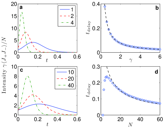
Figure 1: Delay of the superradiant pulse as a function of the decay rate $\gamma$ (upper panels) and the atom number $N$ (lower panels). (a) Intensity $I(t)$ of the light pulse for $N=20$ atoms and three different values of $\gamma$. (b) Delay time $t_{\rm delay}$ as a function of $\gamma$ for $N=20$ atoms. (c) Intensity $I(t)$ of the light pulse for $\gamma=1$ and three different values of $N$. (d) Delay time $t_{\rm delay}$ as a function of the atom number $N$ and $\gamma=1$. The dashed line is the mean-field prediction (8).

As the light intensity (5) is the essential observable measured in experiments, we briefly review some properties of the emitted superradiant pulse, in particular the time scale of the emission. Assuming that initially all atoms are in the excited state, each atom can spontaneously emit a photon. However, the emitted photons also stimulate the emission of further photons from the remaining excited atoms. Thus, the number of photons rapidly increases such that light is emitted in short intense pulse, as shown in Fig. 1 (a) and (c). The delay time $t_{\rm delay}$, at which the pulse assumes its maximum, obviously depends on the emission rate $\gamma$ as shown in Fig. 1 (b).

Furthermore, the dynamics strongly depends on the quantum noise of the initial quantum state. When all atoms are in the excited state, the quantum uncertainty of the collective atomic variables are given by

$$\Delta J_{x}=\Delta J_{y}=\sqrt{N}.$$ (6)

The quantum shot noise, i.e. the relative uncertainty of the Bloch vector $\mathbf{J}$, thus scales as

$$\frac{|\Delta\mathbf{J}|}{|\mathbf{J}|}\sim\frac{1}{\sqrt{N}}$$ (7)

and vanishes in the classical limit $N\rightarrow\infty$. This noise drives the emission process such that the delay time of the superradiant pulse depends strongly on the atom number $N$. As shown in Fig. 1 (d), the delay time first increases rapidly with $N$ and then decreases again. The delay time can be inferred from a mean-field treatment of the atomic dynamics, taking into account the quantum fluctuations of the initial state (6). This approximation predicts that Gros82

$$t_{\rm delay}=(\gamma N)^{-1}\log N.$$ (8)

The mean-field prediction is compared to the numerically exact results in Fig. 1 (b) and (d), showing a good agreement when the atom number is large enough.

III Driven Superradiant Light Scattering

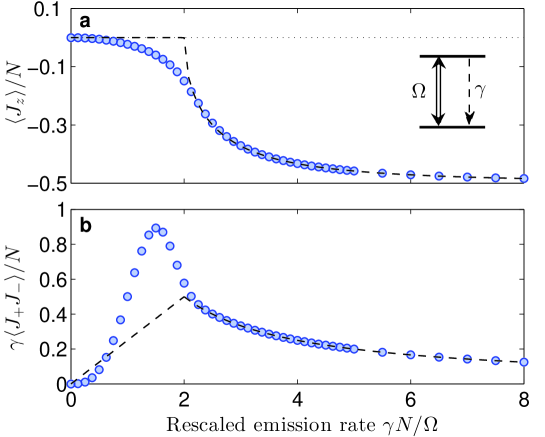
Figure 2: The steady state of the resonantly driven Dicke model. (a) Population imbalance $\langle\hat{J}_{z}\rangle/N$ and (b) intensity of the emitted light (5) as a function of the rescaled emission rate $\gamma N/\Omega$. Circles represent numerical results for $N=20$ atoms and $\Omega=1$, the dashed line is the mean-field prediction (16). The inset in (a) illustrates the system under consideration.

The Dicke model shows a very rich dynamics when an external driving by a classical light field is included. The Hamiltonian describing the coherent driving is given by

$$\hat{H}=-\Delta\hat{J}_{z}-\frac{\Omega}{2}\left(\hat{J}_{+}+\hat{J}_{-}\right),$$ (9)

where $\Omega$ is the Rabi frequency and $\Delta$ is the detuning of the laser frequency with respect to the atomic transition frequency. If the driving is resonant ($\Delta=0$), the Dicke model undergoes a quantum phase transition in the thermodynamic limit $N\rightarrow\infty$. In this limit we can invoke a mean-field approximation, such that the dynamics of the expectation values $J_{z}=\langle\hat{J}_{z}\rangle$ and $J_{\pm}=\langle\hat{J}_{\pm}\rangle$ follows the equations of motion

$$\frac{dJ_{+}}{dt} = -{\rm i}\Delta J_{+}+{\rm i}\Omega J_{z}+\gamma J_{+}J_{z}$$

$$\frac{dJ_{z}}{dt} = {\rm i}\frac{\Omega}{2}(J_{+}-J_{-})-\gamma J_{+}J_{-},$$ (10)

On the resonance, the steady state is given by

$$J_{z} = \left\{\begin{array}[]{l c l}0&\mbox{ for }&2\Omega\leq\gamma N\\ -\sqrt{N^{2}/4-\Omega^{2}/\gamma}&&2\Omega>\gamma N\end{array}\right.$$ (13)

$$J_{+}J_{-} = \left\{\begin{array}[]{l c l}N^{2}/4&\mbox{ for }&2\Omega\leq\gamma N\\ \Omega^{2}/\gamma^{2}&&2\Omega>\gamma N\end{array}\right.$$ (16)

For strong driving or a weak decay, respectively, the population imbalance vanishes exactly. When the decay becomes stronger, $\gamma N>2\Omega$, a phase transition to an ordered state with $\langle\hat{J}_{z}\rangle<0$ takes place. This behavior is shown in Fig. 2 (a), where the population imbalance $\langle\hat{J}_{z}\rangle$ is plotted as a function of the rescaled emission rate $\gamma N/\Omega$. For finite particle number $N$, the transition becomes smeared out and $\langle\hat{J}_{z}\rangle$ is small but non-zero, even for $\gamma N<2\Omega$. The Dicke phase transition can be analyzed fully analytically for arbitrary particle numbers $N$ Garr11 , so we do not go into detail here. An experimental observation of this phase transition has been reported only recently Baum10 .

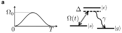
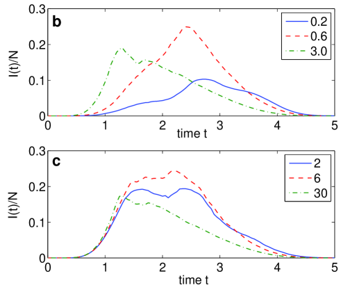
Figure 3: Superradiant Raman scattering by a sample of $N$ $\Lambda$-type atoms. (a) Schematic representation of the scattering process. The driving field $\Omega(t)$ is time-dependent with a pulse length $T$ and maximum value $\Omega_{0}$. (b) The emitted superradiant pulse $I(t)$ for three different values of $\gamma$ and $N=20$. (c) The emitted superradiant pulse $I(t)$ for three different values of $N$ and $\gamma=1$.

In this article, we are primarily interested in the scattering light intensity, which can be viewed as the response of the atomic cloud to the coherent driving. Figure 2 (b) shows the intensity (5) per atom as a function of the emission rate $\gamma$. One observes a clear maximum in the vicinity of the phase transition $\gamma N\approx 2\Omega$. This can be viewed as a stochastic resonance effect. The response of the quantum system assumes its maximum for a specific non-zero coupling to the environment, given by a specific value of $\gamma$. Moreover, the maximum is found if the timescale of the driving $(2\Omega)^{-1}$ is matched to the timescale of the environment coupling $(N\gamma)^{-1}$.

We note that the scattered intensity essentially depends on the effective emission rate $\gamma N/\Omega$. Hence, the observed stochastic resonance is also present in the scattering of a single atom and when the atom number $N$ is varied. This effect is similar to the stochastic resonance observed in systems described by the Bloch equations, which are also governed by the competition of excitation and relaxation Viol00 ; 08stores ; 09srlong . Stochastic resonance effects in composite classical systems and their dependence on the number of constituents has been analyzed in Marc96 .

IV Stochastic Resonance in Periodically Driven Systems

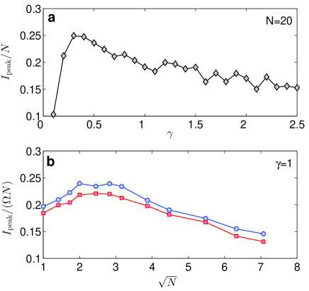
Figure 4: Stochastic resonance in superradiant Raman scattering: The peak intensity per atom of the emitted pulse assumes a maximum for a specific non-zero value of (a) the coupling rate to the environment $\gamma$ and (b) the magnitude of the quantum uncertainty $\sqrt{N}$. The remaining parameters are $\Omega_{0}=1$ (blue circles) and $\Omega_{0}=2$ (red squares), $\Delta=1$, $T=5$ and (a) $N=20$ and (b) $\gamma=1$, respectively. Solid lines are shown to guide the eye.

Superradiant light emission is essentially started by quantum fluctuations such that its timescale is determined by the quantum uncertainty $N^{1/2}$. Therefore we can identify another, much more subtle stochastic resonance effect.

We consider superradiant Raman scattering of a light pulse by a dense sample of three-level atoms as shown in Fig. 3 (a). The atoms emit light collectively, when they decay from the excited state $|e\rangle$ to the ground state $|g\rangle$ as described by the Dicke master equation (4). However, we assume that they are initially prepared in a metastable state $|s\rangle$, which is coupled to the excited state by a classical light pulse,

$$\hat{H}=-\frac{\Delta}{2}\left(\hat{J}_{ss}+\hat{J}_{ee}\right)-\frac{\Omega(t)}{2}\left(\hat{J}_{se}+\hat{J}_{es}\right).$$ (17)

The collective operators used here are defined as usual

$$\hat{J}_{ab}=\frac{1}{N}\sum_{j}|a\rangle_{j}\left\langle b\right|_{j}\,,$$ (18)

where $a$ and $b$ label one of the atomic states $|s\rangle$ or $|e\rangle$. For simplicity, we assume that the input pulse is given by $\Omega(t)=\Omega_{0}\sin(\pi t/T)^{2}$ in the interval $t\in[0,T]$. We solve the master equation numerically using the Monte Carlo wave function method Dali92 ; Carm93 averaging over 500 ($N\leq 15$) resp. 100 ($N\geq 20$) random trajectories.

Figure 3 (a) and (b) show the emitted light pulse for different values of $\gamma$ and the atom number $N$. In both cases, we observe that the peak intensity is largest for intermediate values of $\gamma$ or $N$, respectively. Obviously, the peak intensity is rather small if the emission rate $\gamma$ and the atom number $N$ are small. In this case the emission is too weak and most atoms remain in the initial state $|s\rangle$. However, if $\gamma$ or $N$ are too large, then the emission starts ’too early’, long before the driving $\Omega(t)$ has reached its maximum. Also in this case, the peak intensity is limited.

This is further analyzed in Fig. 4, where the peak intensity per atom is plotted as a function of (a) the emission rate $\gamma$ and $(b)$ the atom number $N$. In both cases we observe a clear maximum when $\gamma$ or $N$ assume intermediate values, such that the time scale of the superradiant emission matches the timescale of the driving. The second case is particularly interesting, as the maximum is found for a specific non-zero strength of the quantum uncertainty $N^{1/2}$. The observed stochastic resonance is thus a genuine quantum effect, as it is observed in terms of the quantum shot noise.

V Conclusion

In this article we have analyzed different stochastic resonance effects in superradiant light scattering. We have identified a genuine quantum stochastic resonance, where the response of the atomic sample to an external driving assumes its maximum for a specific non-zero strength of the quantum shot noise $N^{-1/2}$. The response is quantified by the scattered light intensity per atom or its peak value, respectively.

The mechanism generating the stochastic resonance is a matching of the timescales of the driving and the superradiant emission. The latter depends on the emission rate $\gamma$, but also on the quantum shot noise of the sample, as the the emission process is essentially started by quantum fluctuations. Thus we can observe a maximum of the response, the stochastic resonance, in terms of both the coupling rate to the environment $\gamma$ and the quantum uncertainty $N^{1/2}$.

References

- (1) Benzi R, Sutera A and Vulpiani A (1981) J. Phys. A: Math. Gen. 14 L453
- (2) Wiesenfeld K and Moss F (1995) Nature (London) 373 33
- (3) Dykman M I, Luchinsky D G, Mannella R, McClintock P V E, Stein N D and Stocks N G (1995) Nuovo Cimento D 17 661
- (4) Gammaitoni L, Hänggi P, Jung P and Marchesoni F (1998) Rev. Mod. Phys. 70 223
- (5) Wellens T, Shatokhin V and Buchleitner A (2004) Rep. Prog. Phys. 67 45
- (6) Löfstedt R and Coppersmith S N (1994) Phys. Rev. Lett. 72 1947
- (7) Wellens T and Buchleitner A (2000) Phys. Rev. Lett. 84 5118
- (8) Huelga S F and Plenio M B (2007) Phys. Rev. Lett. 98 170601
- (9) Viola L, Fortunato E M, Lloyd S, Tseng C H and Cory D G (2000) Phys. Rev. Lett. 84 5466
- (10) Witthaut D, Trimborn F and Wimberger S (2008) Phys. Rev. Lett. 101 200402
- (11) Witthaut D, Trimborn F and Wimberger S (2009) Phys. Rev. A 79 033621
- (12) Witthaut D, Trimborn F, Hennig H, Kordas G, Geisel T and Wimberger S (2011) Phys. Rev. A 83 063608
- (13) Trimborn F, Witthaut D, Hennig H, Kordas G, Geisel T and Wimberger S (2011) Eur. Phys. J. D 63 63
- (14) Gross M and Haroche S (1982) Phys. Rep. 93 301 (1992) Phys. Rev. Lett. 68 580
- (15) Dicke R H (1954) Phys. Rev. 93 99
- (16) Garraway B M (2011) Phil. Trans. R. Soc. A 369 1137
- (17) Baumann K, Guerlin C, Brennecke F and Esslinger T (2010) Nature (London) 464 1301
- (18) Marchesoni F, Gammaitoni L and Bulsara A R (1996) Phys. Rev. Lett. 76 2609
- (19) Dalibard J, Castin Y and Mølmer K (1992) Phys. Rev. Lett. 68 580
- (20) Carmichael H J (1993) An Open Systems Approach to Quantum Optics (Springer, Berlin)