Abstract

For the coherently driven $\Lambda$-type three-level systems the general ready-to-calculate expression for the susceptibility tensor at the frequency of the weak probe field is obtained for the arbitrary polarization of the strong coupling laser field and arbitrary values of the angular momenta of resonant atomic levels. The dependence of the relative difference in the group velocities of the two polarization components of the probe field on the polarization of the coupling field is studied.

1 Introduction

The phenomenon of the electromagnetically induced transparency (EIT), when the optical properties of the media for the weak probe field are coherently controlled by the strong coupling field, has been extensively studied in the recent years and provided a number of attractive applications [1]. The most prominent feature of EIT is a spectacular reduction of the group velocity of light pulses in the resonant media [2, 3]. The strong coupling field with the definite polarization produces also the optical anisotropy for the probe field, which reveals itself in the electromagnetically induced birefringence and polarization rotation of the probe field [4, 5]. Among the most promising applications of EIT is the implementation of quantum memory [6, 7, 8]. Such memory based on the controlled adiabatic deceleration and acceleration of single-photon pulses in the resonant media was suggested in [9, 10], and soon the possibility of storage of light pulses was realized in rubidium vapor in the experiment [11]. The recent experiments [12, 13, 14] on EIT-based quantum memory demonstrate the continuously improving efficiency and fidelity. There are different ways to encode the single-photon qubit, for example, in two spectral components of the photon pulse, as it was recently proposed in [15], but the most natural way for qubit encoding is provided by the photon two polarization degrees of freedom, as it was implemented in the experiments [12, 13]. To store the photon polarization qubit its both polarization components must be effectively stopped in the medium, however the group velocities of these two components may differ essentially due to the optical anisotropy induced by the polarization of the coupling field. The experiments on EIT are performed on the the three-level $\Lambda$-type systems with degenerate levels, which are in many cases the hyperfine structure components of alkali atoms degenerate in the projections of the atomic total angular momentum on the quantization axis. The theoretical treatment of EIT on such levels involves the solution of the equations for the atomic density matrix and the number of elements of this matrix increases drastically with the increase of the level angular momentum values. The objective of the present article is to obtain the general expression for the linear susceptibility tensor at the frequency of the probe field, which describes the polarization properties of EIT, and to study the dependence of the relative difference in the group velocities of the two polarization components of the probe field on the polarization of the coupling field. The essential point about this expression is that the susceptibility tensor may be easily calculated by means of standard matrix operations for the arbitrary polarization of the driving field and for the arbitrary values of the level angular momenta.

2 Basic equations and relations

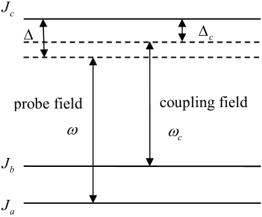
Figure 1: The level diagram.

We consider the weak probe field propagating along the sample axis $Z$ with the carrier frequency $\omega$, which is in resonance with the frequency $\omega_{0}$ of an optically allowed transition $J_{a}\rightarrow J_{c}$ between the ground state $J_{a}$ and the excited state $J_{c}$, and the strong coherent coupling field propagating in the same direction with the carrier frequency $\omega_{c}$, which is in resonance with the frequency $\omega_{c0}$ of an optically allowed transition $J_{b}\rightarrow J_{c}$ between the long-lived state $J_{b}$ and the same excited state $J_{c}$ (Fig.1). Here $J_{a}$, $J_{b}$ and $J_{c}$ are the values of the angular momenta of the levels. The electric field strength of the coupling field (inside the sample as well as outside) and that of the probe field incident on the sample border $z=0$ may be put down as follows:

$$\textbf{E}_{c}=e_{c}\textbf{l}_{c}e^{-i\omega_{c}(t-z/c)}+c.c.,$$ (1)

$$\textbf{E}_{0}=\textbf{e}_{0}e^{-i\omega(t-z/c)}+c.c.,$$ (2)

where $e_{c}$ and $\textbf{l}_{c}$ are the constant amplitude and the unit polarization vector of the coupling field, while $\textbf{e}_{0}$ is the constant vector amplitude of the incident probe field. At some sample point $z$, where the vector amplitude of the probe field is e, the evolution of the atomic slowly-varying density matrix $\hat{\rho}$ in the rotating-wave approximation is described by the equation:

$$\frac{d\hat{\rho}}{dt}=\frac{i}{2}\left[\hat{V},\hat{\rho}\right]+\left(\frac{d\hat{\rho}}{dt}\right)_{rel},$$ (3)

$$\hat{V}=2(\Delta\hat{P}_{c}+\delta\hat{P}_{b})+\Omega_{c}(\hat{g}_{c}+\hat{g}_{c}^{{\dagger}})+\hat{G}+\hat{G}^{{\dagger}},$$ (4)

$$\hat{g}_{c}=\hat{\textbf{g}}_{c}\textbf{l}_{c}^{*},~{}\hat{G}=(2|d|/\hbar)\hat{\textbf{g}}\textbf{e}^{*}.$$ (5)

Here $\Delta=\omega-\omega_{0}$ and $\Delta_{c}=\omega_{c}-\omega_{c0}$ are the frequency detunings from resonance of the probe and of the coupling fields, while $\delta=\Delta-\Delta_{c}$, $\hat{P}_{\alpha}$ is the projector on the subspace of the atomic level $J_{\alpha}$ ($\alpha=a,b,c$), $\Omega_{c}=2|d_{c}|e_{c}/\hbar$ is the reduced Rabi frequency for the coupling field, $d=d(J_{a}J_{c})$ and $d_{c}=d(J_{b}J_{c})$ being the reduced matrix elements of the electric dipole moment operator for the transitions $J_{a}\rightarrow J_{c}$ and $J_{b}\rightarrow J_{c}$, while $\hat{\textbf{g}}$ and $\hat{\textbf{g}}_{c}$ are the dimensionless electric dipole moment operators for the transitions $J_{a}\rightarrow J_{c}$ and $J_{b}\rightarrow J_{c}$. The matrix elements of the circular components $\hat{g}_{q}$ and $\hat{g}_{cq}$ ($q=0,\pm 1$) of these vector operators are expressed through Wigner 3J-symbols [16]:

$$(\hat{g}_{q})^{ac}_{m_{a}m_{c}}=(-1)^{J_{a}-m_{a}}\left(\matrix{J_{a}&1&J_{c}\cr-m_{a}&q&m_{c}}\right),$$ (6)

$$(\hat{g}_{cq})^{bc}_{m_{b}m_{c}}=(-1)^{J_{b}-m_{b}}\left(\matrix{J_{b}&1&J_{c}\cr-m_{b}&q&m_{c}}\right).$$ (7)

Finally, the term $(d\hat{\rho}/dt)_{rel}$ in the equation (3) describes the irreversible relaxation. Initially the atoms are at the ground state $a$ the atomic density matrix being

$$\hat{\rho}(0)=\hat{\rho}_{a}.$$

Generally the atoms are at the equilibrium ground state with equally populated Zeeman sublevels, however they may be prepared at some special state [13]. In the linear approximation for the probe field we obtain from the equations (3)-(4) for the elements of the steady-state ($d\hat{\rho}/dt=0$) atomic density matrix the following relations:

$$(\gamma-i\Delta)\hat{\rho}^{ca}=\frac{i}{2}\left(\Omega_{c}\hat{g}_{c}^{{\dagger}}\hat{\rho}^{ba}+\hat{G}^{{\dagger}}\hat{\rho}_{a}\right),$$ (8)

$$(\Gamma-i\delta)\hat{\rho}^{ba}=\frac{i}{2}\Omega_{c}\hat{g}_{c}\hat{\rho}^{ca},$$ (9)

where

$$\hat{\rho}^{\alpha\beta}=\hat{P}_{\alpha}\hat{\rho}\hat{P}_{\beta},~{}\alpha,\beta=a,b,c,$$

while the irreversible relaxation is simply characterized by the two real relaxation rates – $\gamma$ for the optically allowed transition $J_{a}\rightarrow J_{c}$ and $\Gamma$ for the optically forbidden transition $J_{a}\rightarrow J_{b}$:

$$\left(\frac{d\hat{\rho}}{dt}\right)_{rel}^{ca}=-\gamma\hat{\rho}^{ca},~{}\left(\frac{d\hat{\rho}}{dt}\right)_{rel}^{ba}=-\Gamma\hat{\rho}^{ba}.$$

From (8)-(9) it follows immediately:

$$\hat{\rho}^{ca}=\frac{i}{2(\gamma-i\Delta)}\hat{U}^{-1}\hat{G}^{{\dagger}}\hat{\rho}_{a},$$ (10)

where

$$\hat{U}=\hat{P}_{c}+\frac{\Omega_{c}^{2}}{4(\gamma-i\Delta)(\Gamma-i\delta)}\hat{g}_{c}^{{\dagger}}\hat{g}_{c}.$$ (11)

The medium polarization component at point $z$

$$\textbf{P}=\textbf{p}e^{-i\omega t}+c.c.$$

with the frequency $\omega$ of the probe field is expressed through the density matrix $\hat{\rho}^{ca}$ defined by (10)-(11):

$$\textbf{p}=n_{0}|d|Tr_{A}\left\{\hat{\textbf{g}}\hat{\rho}^{ca}\right\},$$ (12)

where $n_{0}$ is the concentration of resonant atoms and the trace is carried out over atomic states. With the two orthonormal vectors $\textbf{l}_{i}$ in the polarization plane $XY$ ($\textbf{l}_{j}\textbf{l}_{k}^{*}=\delta_{jk},~{}j,k=1,2$) the equation (12) with an account of (10)-(11) and (5) may be expressed through the susceptibility tensor $\chi_{jk}$:

$$p_{j}=\varepsilon_{0}\sum_{k=1}^{2}\chi_{jk}e_{k},$$ (13)

where

$$\chi_{jk}=\frac{i\chi_{0}}{1-i(\Delta/\gamma)}Tr_{A}\left\{\hat{U}^{-1}\hat{g}_{k}^{{\dagger}}\hat{\rho}_{a}\hat{g}_{j}\right\},$$ (14)

$$\chi_{0}=\frac{n_{0}|d|^{2}}{\varepsilon_{0}\hbar\gamma},~{}\hat{g}_{j}=\hat{\textbf{g}}\textbf{l}_{j}^{*}.$$ (15)

With the introduction of the orthonormal set of eigenvectors $|c_{n}>$ with non-negative eigenvalues $c_{n}^{2}$ of the hermitian operator $\hat{g}_{c}^{{\dagger}}\hat{g}_{c}$:

$$\hat{g}_{c}^{{\dagger}}\hat{g}_{c}|c_{n}>=c_{n}^{2}|c_{n}>,n=1,...,2J_{c}+1,$$

the susceptibility tensor (14) may be transformed to the expression:

$$\chi_{jk}=\frac{i\chi_{0}}{1-i(\Delta/\gamma)}\sum_{n=1}^{2J_{c}+1}\frac{<c_{n}|\hat{g}_{k}^{{\dagger}}\hat{\rho}_{a}\hat{g}_{j}|c_{n}>}{\lambda_{n}},$$ (16)

$$\lambda_{n}=1+\frac{c_{n}^{2}\Omega_{c}^{2}}{4(\gamma-i\Delta)(\Gamma-i\delta)}.$$ (17)

Now let $\chi_{k}$ be the two eigenvalues and

$$\textbf{v}_{k}=\sum_{j=1}^{2}v_{jk}\textbf{l}_{j},~{}k=1,2,$$ (18)

be the corresponding two eigenvectors of the $2\times 2$ susceptibility matrix $\hat{\chi}=\{\chi_{jk}\}$:

$$\hat{\chi}\textbf{v}_{k}=\chi_{k}\textbf{v}_{k},~{}k=1,2.$$

Then, the vector amplitude $\textbf{e}_{0}$ of the incident probe field after the passage of the distance $z$ in the medium is transformed to

$$\textbf{e}=\hat{S}\textbf{e}_{0},~{}\hat{S}=\hat{v}\hat{T}\hat{v}^{-1},$$ (19)

where $\hat{v}=\{v_{jk}\}$ is the $2\times 2$-matrix, defined by the equation (18), while the diagonal matrix $\hat{T}$ is determined by the eigenvalues $\chi_{k}$ of the susceptibility matrix:

$$T_{jk}=\delta_{jk}e^{i(\omega/c)zn_{j}},~{}n_{j}=\sqrt{1+\chi_{j}},$$ (20)

as it may be obtained in a usual way from the Maxwell equation

$$\frac{\partial^{2}\textbf{E}}{\partial z^{2}}-\frac{1}{c^{2}}\frac{\partial^{2}\textbf{E}}{\partial t^{2}}=\frac{1}{\varepsilon_{0}c^{2}}\frac{\partial^{2}\textbf{P}}{\partial t^{2}}$$

for the electric field strength E of the probe field. The intensity $I$ and the $2\times 2$ polarization matrix $\hat{\sigma}=\{\sigma_{jk}\}$ of the probe field after the passage of the distance $z$ in the medium are related to the intensity $I_{0}$ and the polarization matrix $\hat{\sigma}_{0}$ of the incident probe field by the equations:

$$\frac{I}{I_{0}}=tr\left(\hat{S}\hat{\sigma}_{0}\hat{S}^{{\dagger}}\right),~{}\hat{\sigma}=\frac{\hat{S}\hat{\sigma}_{0}\hat{S}^{{\dagger}}}{tr\left(\hat{S}\hat{\sigma}_{0}\hat{S}^{{\dagger}}\right)},$$ (21)

where transformation matrix $\hat{S}$ is defined by (19)-(20).

Figure 2: The imaginary part of susceptibility $Im(\chi_{xx}/\chi_{0})$ (dashed line) and $Im(\chi_{yy}/\chi_{0})$ (solid line) versus dimensionless frequency detuning $\Delta/\gamma$ on the transitions with $J_{a}=0$, $J_{b}=J_{c}=1$ at $\Omega_{c}/\gamma=1$, $\Gamma/\gamma=0.01$ and $\textbf{l}_{c}=\textbf{l}_{x}$, $\Delta_{c}=0$.

The electromagnetically induced transparency is associated with the significant reduction of the group velocity of the probe field due to the steep dispersion at the transparency window. Since the dispersion is different for the two polarization components of the probe field, these two components will be differently slowed down in the medium. Let us calculate the relative difference of the group velocities for these two polarization components. For the observation of the electromagnetically induced transparency the coupling field must be strong enough:

$$\Omega_{c}^{2}\gg\Gamma\gamma.$$

Then, close to the two-photon resonance $\delta\leq\Gamma$ the general formula (16)-(17) for the susceptibility tensor is simplified to the following expression:

$$\chi_{jk}=\frac{4\chi_{0}\gamma}{\Omega_{c}^{2}}\left(\delta+i\Gamma\right)a_{jk},$$ (22)

where

$$a_{jk}=\sum_{n}\frac{<c_{n}|\hat{g}_{k}^{{\dagger}}\hat{\rho}_{a}\hat{g}_{j}|c_{n}>}{c_{n}^{2}},$$ (23)

is a hermitian $2\times 2$ matrix. The summation in (23) is carried out over all eigenvectors $|c_{n}>$ of the operator $\hat{g}_{c}^{{\dagger}}\hat{g}_{c}$ with non-zero eigenvalues $c_{n}^{2}>0$. The two eigenvectors $\textbf{v}_{k}$ (18) of the susceptibility matrix $\{\chi_{jk}\}$ coincide with the two orthonormal eigenvectors of the hermitian matrix $\{a_{jk}\}$, while its eigenvalues

$$\chi_{k}=\frac{4\chi_{0}\gamma}{\Omega_{c}^{2}}\left(\delta+i\Gamma\right)a_{k},$$

are expressed through the real eigenvalues $a_{k}$ of matrix $\{a_{jk}\}$. The group velocities $V^{gr}_{k}$ of the two probe field components polarized along eigenvectors $\textbf{v}_{k}$ are determined by the refraction indices $n^{\prime}_{k}=Re\left(\sqrt{1+\chi_{k}}\right)$:

$$V^{gr}_{k}=\frac{c}{n^{\prime}_{k}+\omega(dn^{\prime}_{k}/d\omega)}.$$

Since $|\chi_{k}|\ll 1$, in the case of steep dispersion

$$\chi_{0}\gamma\omega\gg\Omega_{c}^{2},$$

we obtain for the group velocities:

$$V^{gr}_{k}=\frac{c}{n^{gr}_{k}},~{}n^{gr}_{k}=\frac{2\chi_{0}\gamma\omega a_{k}}{\Omega_{c}^{2}}.$$ (24)

The relative difference of these two group velocities

$$\varepsilon=\frac{V^{gr}_{2}-V^{gr}_{1}}{V^{gr}_{2}}=1-\frac{a_{2}}{a_{1}}$$ (25)

is determined by the difference of the two eigenvalues $a_{k}$ of matrix $\{a_{jk}\}$, $a_{1}$ being the largest of them and the group velocity $V^{gr}_{1}$ of the probe field component polarized along the corresponding eigenvector $\textbf{v}_{1}$ being the smallest of two.

3 Discussion

Figure 3: The real part of susceptibility $Re(\chi_{xx}/\chi_{0})$ (dashed line) and $Re(\chi_{yy}/\chi_{0})$ (solid line) versus dimensionless frequency detuning $\Delta/\gamma$ on the transitions with $J_{a}=0$, $J_{b}=J_{c}=1$ at $\Omega_{c}/\gamma=1$, $\Gamma/\gamma=0.01$ and $\textbf{l}_{c}=\textbf{l}_{x}$, $\Delta_{c}=0$.

The $(2J_{b}+1)\times(2J_{c}+1)$ matrices $\hat{g}_{c}$ and $(2J_{a}+1)\times(2J_{c}+1)$ matrices $\hat{g}_{j}$ ($j=1,2$) of the electric dipole moment operators may be easily calculated for any reasonable values of the angular momenta $J_{a}$, $J_{b}$ and $J_{c}$ of the resonant atomic levels using the known formulae for Wigner 3J-symbols, and further calculations of the susceptibility tensor $\hat{\chi}$ (14) and of the transformation matrix $\hat{S}$ (19), involving standard matrix operations, are rather simple. In the following numerical calculations we shall assume the coupling field to be rather strong: $\Omega_{c}/\gamma=1$ and exactly resonant $\Delta_{c}=0$, and the relaxation rate of the forbidden transition to be rather small: $\Gamma/\gamma=0.01$, as it is the case for the electromagnetically induced transparency, while the atoms are initially at the equilibrium state:

$$\hat{\rho}_{a}=\frac{\hat{P}_{a}}{2J_{a}+1}.$$

We shall also consider the linearly polarized coupling field, then without loss of generality its polarization vector may be directed along the Cartesian axis $X$: $\textbf{l}_{c}$ = $\textbf{l}_{x}$, and we shall choose the Cartesian basis $\textbf{l}_{1}=\textbf{l}_{x}$, $\textbf{l}_{2=}\textbf{l}_{y}$ in the polarization plane $XY$ for the calculation of the elements of the susceptibility tensor. With this choice of the Cartesian basis the polarization matrix $\hat{\sigma}$ (21) of the probe field may be expressed through the Stokes parameters $\xi_{n}$ ($n=1,2,3$):

$$\sigma=\frac{1}{2}\left(\matrix{1+\xi_{3}&\xi_{1}-i\xi_{2}\cr\xi_{1}+i\xi_{2}&1-\xi_{3}}\right),$$

$$P=\sqrt{\xi_{1}^{2}+\xi_{2}^{2}+\xi_{3}^{2}}$$

being the total degree of polarization,

$$P_{l}=\sqrt{\xi_{1}^{2}+\xi_{3}^{2}}$$

being the degree of linear polarization, and

$$P_{c}=|\xi_{2}|$$

being the degree of circular polarization.

Figure 4: The relative intensity $I/I_{0}$ (dashed line) and the degree of polarization $P$ (solid line) of the initially unpolarized probe field versus dimensionless medium depth $z/L$ ($L=1/k\chi_{0}$) on the transitions with $J_{a}=0$, $J_{b}=J_{c}=1$ at $\Omega_{c}/\gamma=1$, $\Gamma/\gamma=0.01$ and $\textbf{l}_{c}=\textbf{l}_{x}$, $\Delta=\Delta_{c}=0$.

Let us consider the transitions with the low values of angular momenta $J_{a}=0$, $J_{b}=J_{c}=1$, which may be realized in thallium vapor for example. With the linear polarization $\textbf{l}_{c}$ = $\textbf{l}_{x}$ of the coupling field the susceptibility tensor becomes diagonal in the Cartesian basis. The dependencies of the imaginary $Im(\chi_{xx}/\chi_{0})$, $Im(\chi_{yy}/\chi_{0})$ and real $Re(\chi_{xx}/\chi_{0})$, $Re(\chi_{yy}/\chi_{0})$ parts of the susceptibility eigenvalues versus the dimensionless frequency detuning $\Delta/\gamma$, obtained from the calculations according to the formula (16), are presented in the Figures 2 and 3. As it follows from these dependencies the strong linearly polarized (along the axis $X$) coupling field opens the ”transparency window” (solid line) for the polarization component of the probe field linearly polarized in the perpendicular direction (along the axis $Y$), while for the component of the probe field collinearly polarized with the coupling field (along the axis $X$) this ”window” remains shut (dashed line), which gives rise to rather strong dichroism for the resonant ($\Delta=0$) probe field. This happens because the $X$-polarized component of the probe field interacts with a single substate

$$|c_{x}>=\frac{1}{\sqrt{2}}\left(|m_{c}=-1>-|m_{c}=1>\right)$$

of the excited level $c$, which is not affected by the coupling field:

$$\hat{g}_{c}|c_{x}>=0.$$

For the initially unpolarized probe field:

$$\hat{\sigma_{0}}=\frac{1}{2}\left(\matrix{1&0\cr 0&1}\right),$$

the dependencies of its relative intensity $I/I_{0}$ (dashed line) and the degree of polarization $P$ (solid line) versus the dimensionless medium depth $z/L$, where $L=1/k\chi_{0}$, are presented in the Figure 4. As it may be seen in this figure, the probe field becomes almost fully polarized with the degree of polarization $P=0.96$ (linearly along the axis $Y$), while its intensity is reduced by the factor of 0.19.

Figure 5: The imaginary part of susceptibility $Im(\chi_{xx}/\chi_{0})$ (dashed line) and $Im(\chi_{yy}/\chi_{0})$ (solid line) versus dimensionless frequency detuning $\Delta/\gamma$ on the transitions with $J_{a}=1$, $J_{b}=J_{c}=2$ at $\Omega_{c}/\gamma=1$, $\Gamma/\gamma=0.01$ and $\textbf{l}_{c}=\textbf{l}_{x}$, $\Delta_{c}=0$.

Let us now consider the transitions with larger values of angular momenta $J_{a}=1$, $J_{b}=J_{c}=2$, which were employed in the experiment [4] performed in ${}^{87}Rb$ vapor. For the linear polarization $\textbf{l}_{c}$ = $\textbf{l}_{x}$ of the coupling field the dependencies of the imaginary $Im(\chi_{xx}/\chi_{0})$, $Im(\chi_{yy}/\chi_{0})$ and real $Re(\chi_{xx}/\chi_{0})$, $Re(\chi_{yy}/\chi_{0})$ parts of the susceptibility eigenvalues versus the dimensionless frequency detuning $\Delta/\gamma$ are presented in the Figures 5 and 6. In this case the ”transparency windows” are open for both polarization components of the probe field, however, that for the $Y$-component (solid line), perpendicular to the coupling field, is larger than for the $X$-component (dashed line), collinear with the coupling field. In the case of large values of the angular momenta the dichroism is less than in the case of small ones, as it may be seen in the Figure 7. When the degree of polarization of the initially unpolarized probe field attains the value of 0.5 its intensity is reduced by the factor of 0.17.

Figure 6: The real part of susceptibility $Re(\chi_{xx}/\chi_{0})$ (dashed line) and $Re(\chi_{yy}/\chi_{0})$ (solid line) versus dimensionless frequency detuning $\Delta/\gamma$ on the transitions with $J_{a}=1$, $J_{b}=J_{c}=2$ at $\Omega_{c}/\gamma=1$, $\Gamma/\gamma=0.01$ and $\textbf{l}_{c}=\textbf{l}_{x}$, $\Delta_{c}=0$.

Figure 7: The relative intensity $I/I_{0}$ (dashed line) and the degree of polarization $P$ (solid line) of the initially unpolarized probe field versus dimensionless medium depth $z/L$ ($L=1/k\chi_{0}$) on the transitions with $J_{a}=1$, $J_{b}=J_{c}=2$ at $\Omega_{c}/\gamma=1$, $\Gamma/\gamma=0.01$ and $\textbf{l}_{c}=\textbf{l}_{x}$, $\Delta=\Delta_{c}=0$.

Figure 8: The dependence of relative difference $\varepsilon=(V^{gr}_{2}-V^{gr}_{1})/V^{gr}_{2}$ in the group velocities of the two polarization components of the probe field on the ellipticity parameter $\alpha$ of the coupling field on the transitions with $J_{a}=J_{c}=1$, $J_{b}=2$.

The relative difference $\varepsilon$ in the group velocities of the two polarization components of the probe field (25) depends only on the values of total angular momenta of resonant levels, on the initial atomic state and on the polarization of the coupling field. Let us consider the coupling field with arbitrary elliptic polarization in the plane $XY$:

$$l_{cq}=\cos\alpha\delta_{q,-1}-\sin\alpha\delta_{q,1},$$

where parameter $\alpha$ defines the ratio of the lengthes $a_{y}$ and $a_{x}$ of the axes of polarization ellipse along the axes $Y$ and $X$ according to the relation

$$\left|\tan\left(\alpha-\frac{\pi}{4}\right)\right|=\frac{a_{y}}{a_{x}},$$

while the sign of $\tan(\alpha-\pi/4)$ determines the direction of rotation of the pulse electric field vector in the plane $XY$. For the atoms at initially equilibrium state and with the fixed values of the level angular momenta the relative difference in the group velocities $\varepsilon$ depends only on the ellipticity parameter $\alpha$ of the coupling field. An example of such dependence for the levels with the angular momenta $J_{a}=J_{c}=1$, $J_{b}=2$, employed in the experiment [13], is presented in the Figure 8. The maximum difference in the group velocities $\varepsilon=0.625$ is obtained with the circularly polarized coupling field ($\alpha=0,\pi/2$), while the minimum difference $\varepsilon=0.125$ is obtained with the linearly polarized coupling field ($\alpha=\pi/4$). In the case of circularly polarized coupling field the polarization component with the larger group velocity is circularly polarized in the same direction as the coupling field, while the polarization component with the smaller group velocity is circularly polarized in the direction opposite to that of the coupling field. In the case of linearly polarized coupling field the polarization component with the smaller group velocity is linearly polarized in same direction as the coupling field, while the polarization component with the larger group velocity is linearly polarized in the direction perpendicular to that of the coupling field. In the experiment [13] the coupling field was linearly polarized in the direction of propagation of the probe field: $l_{cq}=\delta_{q,0}$ ($\pi$-polarized), while it propagated in the perpendicular direction, and the atoms were prepared at the pure Zeeman state $|J_{a}=1,m_{a}=0>$ with the zero projection on the quantization axis. Under such conditions we obtain for the tensor (23): $a_{jk}=1.667\delta_{jk}$, so that the group velocity of the probe pulse in this case does not depend on its polarization. For the unprepared atoms, which are initially in the equilibrium state with equally populated Zeeman sublevels, we obtain $a_{jk}=0.972\delta_{jk}$, so that in this case the group velocity of the probe pulse also does not depend on its polarization.

4 Conclusions

In the present article the $\Lambda$-type three-level systems with degenerate levels coherently driven by the strong laser field are considered. The general expression for the susceptibility tensor at the frequency of the weak probe field is obtained for the arbitrary polarization of the strong coupling laser field and arbitrary values of the momenta $J_{a}$, $J_{b}$, $J_{c}$ of resonant atomic levels. The numerical calculations, based on this expression, may be easily performed by means of standard matrix operations for any reasonable values of angular momenta. Sample calculations for the transitions with $J_{a}=0$, $J_{b}=J_{c}=1$ and $J_{a}=1$, $J_{b}=J_{c}=2$, which are employed in the experiments with atomic vapors, were carried out. It was shown, that the depth of the ”transparency window” for the resonant probe field depends on its polarization providing rather strong dichroism. Such dependence is greater for the low values of angular momenta $J_{a}=0$, $J_{b}=J_{c}=1$ and it is muffled for larger values $J_{a}=1$, $J_{b}=J_{c}=2$. The general expression for the relative difference in the group velocities of the two polarization components of the probe field is obtained. This difference depends on the values of total angular momenta of resonant levels, on the initial atomic state and on the polarization of the coupling field. Such dependence on the ellipticity parameter of the coupling field for the transitions with $J_{a}=J_{c}=1$, $J_{b}=2$, studied numerically, revealed rather a wide range of variation of this relative difference – from 0.625 with the circularly polarized coupling field to 0.125 with the linearly polarized one.

Acknowledgements

Authors are indebted for financial support of this work to Russian Ministry of Science and Education (grant 2.2407.2011).

References

- [1] Fleischhauer M, Imamoglu A and Marangos J 2005 Rev.Mod.Phys. 77 633
- [2] Kash M et al 1999 Phys.Rev.Lett. 82 5229
- [3] Budker D et al 1999 Phys.Rev.Lett. 83 1767
- [4] Li S et al 2006 Phys.Rev.A 74 033821
- [5] Zhang H, Zhou L and Sun C 2009 Phys.Rev.A 80 013812
- [6] Lvovsky A, Sanders B and Tittel W 2009 Nature Photonics 3 706
- [7] Simon C et al 2010 Eur.Phys.J. 58 1
- [8] Himsworth M et al 2011 Appl.Phys.B 103 579
- [9] Lukin M, Yelin S and Fleischhauer M 2000 Phys.Rev.Lett. 84 4232
- [10] Fleischhauer M and Lukin M 2000 Phys.Rev.Lett. 84 5494
- [11] Phillips D et al 2001 Phys.Rev.Lett. 86 783
- [12] Cho Y and Kim Y 2010 Optics Express 18 25786
- [13] Riedl S et al 2012 Phys.Rev.A 85 022318
- [14] Zhou S et al 2012 Optics Express 20 24124
- [15] Viscor D et al 2012 Phys.Rev.A 86 053827
- [16] Sobelman I 1972 Introduction to the Theory of Atomic Spectra (New York: Pergamon)