Semileptonic decays $B\to D^{(*)}l\nu$ in the perturbative QCD factorization approach

Abstract

Abstract     In this paper, we study the $B\to D^{(*)}l^{-}\bar{\nu}_{\rm l}$ semileptonic decays and calculate the branching ratios ${\cal B}(B\to D^{(*)}l^{-}\bar{\nu}_{\rm l})$ and the ratios $R(D^{(*)})$ and $R_{\rm D}^{\rm l,\tau}$ by employing the perturbative QCD (pQCD) factorization approach. We find that (a) for $R(D)$ and $R(D^{*})$ ratios, the pQCD predictions are $R(D)=0.430^{+0.021}_{-0.026}$, $R(D^{*})=0.301\pm 0.013$ and agree well with BaBar’s measurements of $R(D^{(*)})$; (b) for the newly defined $R_{\rm D}^{\rm l}$ and $R_{\rm D}^{\rm\tau}$ ratios, the pQCD predictions are $R_{\rm D}^{\rm l}=0.450^{+0.064}_{-0.051}$ and $R_{\rm D}^{\rm\tau}=0.642^{+0.081}_{-0.070}$, which may be more sensitive to the QCD dynamics of the considered semileptonic decays than $R(D^{(*)})$ and should be tested by experimental measurements.

Key Words B meson semileptonic decays; The pQCD factorization approach; Form factors; Branching ratios

1     Introduction

The semileptonic decays $B\to D\tau\bar{\nu}_{\rm\tau}$ and $B\to D^{*}\tau\bar{\nu}_{\rm\tau}$ have been previously measured by both BaBar and Belle Collaborations with $3.8\sigma$ and $8.1\sigma$ significance babar2008 ; belle2007 ; belle2010 . Very recently, the BaBar collaboration with their full data greatly improved their previous analysis and reported their measurements for the relevant branching ratios and the ratios $R(D^{(*)})$ of the corresponding branching ratios prl109-101802 :

$${\cal R}(D)=0.440\pm 0.072,\quad{\cal R}(D^{*})=0.332\pm 0.030,$$ (1)

where the isospin symmetry relations ${\cal R}(D^{0})={\cal R}(D^{+})={\cal R}(D)$ and ${\cal R}(D^{*0})={\cal R}(D^{*+})={\cal R}(D^{*})$ have been imposed, and the statistical and systematic uncertainties have been combined in quadrature. These BaBar results are surprisingly larger than the standard model (SM) predictions as given in Ref. prd85-094025 :

$${\cal R}(D)^{\rm SM} = 0.296\pm 0.016\;,\quad{\cal R}(D^{*})^{\rm SM}=0.252\pm 0.003,$$ (2)

The combined BaBar results disagree with the SM predictions by $3.4\sigma$ prl109-101802 ; bozek-2013 .

Since the report of BaBar measurements, this $R(D^{(*)})$ anomaly has been studied intensively by many authors, for example, in Refs. prl109-071802 ; prd85-114502 ; prl109-161801 ; prd86-054014 ; jhep2013-01054 ; prd86-034027 ; prd86-114037 ; mpla27-1250183 ; Fajfer-1301 ; pich-1301 ; R17 ; R18 . Some authors treat this $3.4\sigma$ deviation as the first evidence for new physics (NP) in semileptonic B meson decays to $\tau$ lepton prl109-161801 ; prd86-054014 ; jhep2013-01054 ; prd86-034027 ; prd86-114037 , such as the NP contributions from the charged Higgs bosons in the Two-Higgs-Doublet models prd86-054014 .

Some other physicists, however, try to interpret the data in the framework of the SM but with their own methods. In Ref. prl109-071802 the authors presented their SM predictions ${\cal R}(D)^{\rm SM}=0.316\pm 0.014$ by using the form factors $F_{\rm 0,+}(q^{\rm 2})$ computed in unquenched lattice QCD by the Fermilab Lattice and MILC collaborationsprd85-114502 . In Refs. mpla27-1250183 ; Kosnik-1301 , furthermore, the authors performed the same kinds of calculations by employing the relativistic quark modelmpla27-1250183 or by maximally employing the experimental information on the relevant form factors from the data of $B\to Dl\bar{\nu}_{\rm l}$ with $l=(e^{-},\mu^{-})$ Kosnik-1301 ; prl104-011802 , and found that:

$${\cal R}(D)^{\rm SM} = 0.315\;[14],\quad{\cal R}(D^{*})^{\rm SM}=0.260\;[14],$$ (3)

$${\cal R}(D)^{\rm SM} = 0.31\pm 0.02\;[17],$$ (4)

It is easy to see that there is a clear discrepancy between these SM predictions for $R(D^{(*)})$ prd85-094025 ; prl109-161801 ; prd85-114502 ; prl109-071802 ; mpla27-1250183 ; Kosnik-1301 and the BaBar’s measurements as listed in Eq. (1).

In Refs. prd86-114025 ; prd87-097501 , we studied the semileptonic decays $B_{\rm(s)}\to(\pi,K,\eta,\eta^{(\prime)},G)(ll,l\nu,\nu\bar{\nu})$ in the pQCD factorization approach ppnp51-85 with the inclusion of the known next-leading-order (NLO) contributions. We found that all known semileptonic decays $B/B_{\rm s}\to P(ll,l\nu,\nu\bar{\nu})$ ( here $P=(\pi,K,\eta,\eta^{(\prime)},etc)$ are light pseudo-scalar mesons) can be understood in the framework of the pQCD factorization approachprd86-114025 ; prd87-097501 .

Motivated by the recent BaBar’s discrepancy of the measured values of $R(D^{(*)})$ from the SM predictions, we here will calculate the branching ratios ${\cal B}(B\to D^{(*)}l^{-}\bar{\nu}_{\rm l})$ and the six R(X)-ratios: the four isospin-unconstrained ratios $R(D^{0})$,$R(D^{*0})$,$R(D^{+})$ and $R(D^{*+})$, as well as the two isospin-constrained ratios $R(D)$ and $R(D^{*})$ in the framework of the SM by employing the pQCD approach again. We will compare the pQCD predictions for the branching ratios and the six $R(X)$ ratios with those as given in Refs. prd85-094025 ; prl109-161801 ; prd85-114502 ; prl109-071802 ; mpla27-1250183 , and the measured values of BaBar Collaboration prl109-101802 . We also define two new ratios of the branching ratios $R_{\rm D}^{\rm l}$ and $R_{\rm D}^{\rm\tau}$, and present the pQCD predictions for new ratios $R_{\rm D}^{\rm l,\tau}$, which will be tested by experimental measurements. Finally, there will be a short summary.

2     Kinematics and the Wave Functions

In the pQCD approach, the lowest order Feynman diagrams for $B\to D^{(*)}l^{-}\bar{\nu}_{\rm l}$ decays are displayed in Fig.1. We discuss kinematics of these decays in the large-recoil (low $q^{\rm 2}$) region where the pQCD factorization approach is applicable to the considered semileptonic decays involving $D$ or $D^{*}$ as the final state mesonli1995 . In the $B$ meson rest frame, we define the $B$ meson momentum $P_{\rm 1}$, the $D^{(*)}$ momentum $P_{\rm 2}$ in the light-cone coordinates asprd67-054028

$$P_{\rm 1}=\frac{m_{\rm B}}{\sqrt{2}}(1,1,0_{\bot}),\quad P_{\rm 2}=\frac{rm_{\rm B}}{\sqrt{2}}(\eta^{+},\eta^{-},0_{\bot}),$$ (5)

The longitudinal polarization vector $\epsilon_{\rm L}$ and transverse polarization vector $\epsilon_{\rm T}$ of the $D^{*}$ meson are given by $\epsilon_{\rm L}=(\eta^{+},-\eta^{-},0_{\bot})/\sqrt{2}$, $\epsilon_{\rm T}=(0,0,1)$ with the factors $\eta^{\pm}=\eta\pm\sqrt{\eta^{\rm 2}-1}$ is defined in terms of the parameter

$$\eta=\frac{1}{2r}\left[1+r^{\rm 2}-\frac{q^{\rm 2}}{m_{\rm B}^{\rm 2}}\right],$$ (6)

where the ratio $r=m_{\rm D}/m_{\rm B}$ or $m_{\rm D^{*}}/m_{\rm B}$, and $q=p_{\rm 1}-p_{\rm 2}$ is the lepton-pair momentum. The momenta of the spectator quarks in $B$ and $D^{(*)}$ mesons are parameterized as

$$k_{\rm 1}=(0,x_{\rm 1}\frac{m_{\rm B}}{\sqrt{2}},k_{1\bot}),\quad k_{\rm 2}=\frac{m_{\rm B}}{\sqrt{2}}(x_{\rm 2}r\eta^{+},x_{\rm 2}r\eta^{-},k_{2\bot}).$$ (7)

Figure 1: The lowest order Feynman diagrams for the semileptonic decays $B\to D^{(*)}l^{-}\bar{\nu}_{\rm l}$ in the pQCD approach, the winding curves are gluons.

For the $B$ meson wave function, we make use of the same one as being used for example in Refs.prd85-094003 ; prd86-011501 ; prd86-114025 , which can be written as the form of

$$\Phi_{\rm B}=\frac{i}{\sqrt{2N_{c}}}(p/_{\rm B}+m_{\rm B})\gamma_{5}\phi_{\rm B}({\bf k_{\rm 1}}).$$ (8)

Here only the contribution of the Lorentz structure $\phi_{\rm B}({\bf k_{\rm 1}})$ is taken into account, since the contribution of the second Lorentz structure $\bar{\phi}_{\rm B}$ is numerically small and has been neglected. We adopted the B-meson distribution amplitude widely used in the pQCD approach ppnp51-85 ; prd86-114025 ; prd87-097501

$$\phi_{\rm B}(x,b) = N_{\rm B}x^{\rm 2}(1-x)^{\rm 2}\mathrm{\exp}\left[-\frac{m_{\rm B}^{\rm 2}\;x^{\rm 2}}{2\omega_{\rm B}^{\rm 2}}-\frac{1}{2}(\omega_{\rm B}b)^{\rm 2}\right],$$ (9)

where the shape parameter $\omega_{\rm B}=0.40$ GeV has been fixed ppnp51-85 from the fit to the $B\to\pi$ form factors derived from lattice QCD and from Light-cone sum rule. In order to analyze the uncertainties of theoretical predictions induced by the inputs, we will set $\omega_{\rm B}=0.40\pm 0.04$ GeV. The normalization factor $N_{\rm B}$ depends on the values of the shape parameter $\omega_{\rm B}$ and the decay constant $f_{\rm B}$ and defined through the normalization relation: $\int_{0}^{1}dx\;\phi_{\rm B}(x,b=0)=f_{\rm B}/(2\sqrt{6})$.

For the pseudoscalar $D$ meson and the vector $D^{*}$ meson, their wave function can be chosen as prd78-014018

$$\Phi_{\rm D}(p,x) = \frac{i}{\sqrt{6}}\gamma_{5}(p/_{\rm D}+m_{\rm D})\phi_{\rm D}(x),$$ (10)

$$\Phi_{\rm D^{*}}(p,x) = \frac{-i}{\sqrt{6}}\left[\epsilon/_{\rm L}(p/_{\rm D^{*}}+m_{\rm D^{*}})\phi^{L}_{\rm D^{*}}(x)+\epsilon/_{\rm T}(p/_{\rm D^{*}}+m_{\rm D^{*}})\phi^{T}_{\rm D^{*}}(x)\right].$$ (11)

For the distribution amplitudes of $D^{(*)}$ meson, we adopt the one as defined in Ref. prd78-014018

$$\phi_{\rm D^{(*)}}(x)=\frac{f_{\rm D^{(*)}}}{2\sqrt{6}}6x(1-x)\left[1+C_{D^{(*)}}(1-2x)\right]\exp\left[-\frac{\omega^{\rm 2}b^{\rm 2}}{2}\right].$$ (12)

From the heavy quark limit, we here assume that $f^{\rm L}_{\rm D^{*}}=f^{\rm T}_{\rm D^{*}}=f_{\rm D^{*}}$, $\phi^{\rm L}_{\rm D^{*}}=\phi^{\rm T}_{\rm D^{*}}=\phi_{\rm D^{*}}$, and set $C_{\rm D}=C_{\rm D^{*}}=0.5,~{}\omega=0.1$ GeV as Ref. prd78-014018 .

3     Form Factors and Semileptonic Decays

For the semileptonic decays $B\to Dl\bar{\nu}_{\rm l}$, the quark level transitions are $b\to cl\bar{\nu}_{\rm l}$ decays with the effective Hamiltonian

$${\cal H}_{\rm eff}(b\to cl\bar{\nu}_{\rm l})=\frac{G_{\rm F}}{\sqrt{2}}V_{\rm cb}\;\bar{c}\gamma_{\mu}(1-\gamma_{5})b\cdot\bar{l}\gamma^{\mu}(1-\gamma_{5})\nu_{\rm l},$$ (13)

where $G_{\rm F}=1.16637\times 10^{-5}$ GeV^-2 is the Fermi-coupling constant.

For $B\to D$ transition, the form factors $F_{\rm 0,+}(q^{\rm 2})$ can be written in terms of $f_{\rm 1,2}(q^{\rm 2})$ as in Ref. prd86-114025 :

$$F_{+}(q^{\rm 2}) = \frac{1}{2}\left[f_{\rm 1}(q^{\rm 2})+f_{\rm 2}(q^{\rm 2})\right],$$

$$F_{0}(q^{\rm 2}) = \frac{1}{2}f_{\rm 1}(q^{\rm 2})\left[1+\frac{q^{\rm 2}}{m_{\rm B}^{\rm 2}-m_{\rm D}^{\rm 2}}\right]+\frac{1}{2}f_{\rm 2}(q^{\rm 2})\left[1-\frac{q^{\rm 2}}{m_{\rm B}^{\rm 2}-m_{\rm D}^{\rm 2}}\right],$$ (14)

with

$$f_{\rm 1}(q^{\rm 2}) = 8\pi m^{\rm 2}_{\rm B}C_{\rm F}\int dx_{\rm 1}dx_{\rm 2}\int b_{\rm 1}db_{\rm 1}b_{\rm 2}db_{\rm 2}\phi_{B}(x_{\rm 1},b_{\rm 1})\phi_{\rm D}(x_{\rm 2},b_{\rm 2})$$ (15)

$$\times\Bigl{\{}\left[2r\left(1-rx_{\rm 2}\right)\right]\cdot h_{\rm 1}(x_{\rm 1},x_{\rm 2},b_{\rm 1},b_{\rm 2})\cdot\alpha_{s}(t_{\rm 1})\cdot\exp\left[-S_{\rm ab}(t_{\rm 1})\right]$$

$$+\left[2r(2r_{\rm c}-r)+x_{\rm 1}r\left(-2+2\eta+\sqrt{\eta^{\rm 2}-1}-\frac{2\eta}{\sqrt{\eta^{\rm 2}-1}}+\frac{\eta^{\rm 2}}{\sqrt{\eta^{\rm 2}-1}}\right)\right]$$

$$\cdot h_{\rm 2}(x_{\rm 1},x_{\rm 2},b_{\rm 1},b_{\rm 2})\cdot\alpha_{\rm s}(t_{\rm 2})\cdot\exp\left[-S_{\rm ab}(t_{\rm 2})\right]\Bigr{\}},$$

$$f_{\rm 2}(q^{\rm 2}) = 8\pi m^{\rm 2}_{\rm B}C_{\rm F}\int dx_{\rm 1}dx_{\rm 2}\int b_{\rm 1}db_{\rm 1}b_{\rm 2}db_{\rm 2}\phi_{\rm B}(x_{\rm 1},b_{\rm 1})\phi_{\rm D}(x_{\rm 2},b_{\rm 2})$$ (16)

$$\times\Bigl{\{}\left[2-4x_{\rm 2}r(1-\eta)\right]\cdot h_{\rm 1}(x_{\rm 1},x_{\rm 2},b_{\rm 1},b_{\rm 2})\cdot\alpha_{\rm s}(t_{\rm 1})\cdot\exp\left[-S_{\rm ab}(t_{\rm 1})\right]$$

$$+\left[4r-2r_{\rm c}-x_{\rm 1}+\frac{x_{\rm 1}}{\sqrt{\eta^{\rm 2}-1}}(2-\eta)\right]\cdot h_{\rm 2}(x_{\rm 1},x_{\rm 2},b_{\rm 1},b_{\rm 2})\cdot\alpha_{\rm s}(t_{\rm 2})\cdot\exp\left[-S_{\rm ab}(t_{\rm 2})\right]\Bigr{\}},\quad$$

where $C_{\rm F}=4/3$ is a color factor, $r_{\rm c}=m_{\rm c}/m_{\rm B}$ with $m_{\rm c}$ is the mass of $c$-quark. The hard functions $h_{\rm 1,2}(x_{\rm i},b_{\rm i})$ come form the Fourier transform and can be written as  prd65-014007 ; prd63-074009

$$h_{\rm 1}(x_{\rm 1},x_{\rm 2},b_{\rm 1},b_{\rm 2}) = K_{\rm 0}(\beta_{\rm 1}b_{\rm 1})\left\{\theta(b_{\rm 1}-b_{\rm 2})I_{\rm 0}(\alpha_{\rm 1}b_{\rm 2})K_{\rm 0}(\alpha_{\rm 1}b_{\rm 1})\right.$$

$$\left.+\theta(b_{\rm 2}-b_{\rm 1})I_{\rm 0}(\alpha_{\rm 1}b_{\rm 1})K_{\rm 0}(\alpha_{\rm 1}b_{\rm 2})\right\}\cdot S_{\rm t}(x_{\rm 2}),$$

$$h_{\rm 2}(x_{\rm 1},x_{\rm 2},b_{\rm 1},b_{\rm 2}) = K_{\rm 0}(\beta_{\rm 2}b_{\rm 1})\left\{\theta(b_{\rm 1}-b_{\rm 2})I_{\rm 0}(\alpha_{\rm 2}b_{\rm 2})K_{\rm 0}(\alpha_{\rm 2}b_{\rm 1})\right.$$ (17)

$$\left.+\theta(b_{\rm 2}-b_{\rm 1})I_{\rm 0}(\alpha_{\rm 2}b_{\rm 1})K_{\rm 0}(\alpha_{\rm 2}b_{\rm 2})\right\}\cdot S_{\rm t}(x_{\rm 2}),$$

where $K_{\rm 0}$ and $I_{\rm 0}$ are modified Bessel functions, while the parameters

$$\alpha_{\rm 1}=m_{B}\sqrt{x_{\rm 2}r\eta^{+}},\quad\alpha_{\rm 2}=m_{\rm B}\sqrt{x_{\rm 1}r\eta^{+}-r^{\rm 2}+r_{\rm c}^{\rm 2}},\quad\beta_{\rm 1}=\beta_{\rm 2}=m_{\rm B}\sqrt{x_{\rm 1}x_{\rm 2}r\eta^{+}},$$ (18)

with $r=m_{D^{(*)}}/m_{\rm B}$. The threshold resummation factor $S_{\rm t}(x_{\rm i})$ is adopted from prd65-014007 , and the Sudakov factor $S_{\rm ab}(t)=S_{\rm B}(t)+S_{\rm M}(t)$ can be found in Refs. prd65-014007 ; prd63-074009 .

With the form factors $F_{\rm 0,+}(q^{\rm 2})$, the differential decay widths of the semileptonic decays $B\to Dl\bar{\nu}_{\rm l}$ can be written as prd79-014013

$$\frac{d\Gamma(B\to Dl\bar{\nu}_{\rm l})}{dq^{\rm 2}} = \frac{G_{F}^{\rm 2}|V_{\rm cb}|^{\rm 2}}{192\pi^{3}m_{\rm B}^{3}}\left(1-\frac{m_{\rm l}^{\rm 2}}{q^{\rm 2}}\right)^{\rm 2}\frac{\lambda^{1/2}(q^{\rm 2})}{2q^{\rm 2}}$$ (19)

$$\cdot\Bigl{\{}3m_{\rm l}^{\rm 2}\left(m_{\rm B}^{\rm 2}-m_{\rm D}^{\rm 2}\right)^{\rm 2}|F_{\rm 0}(q^{\rm 2})|^{\rm 2}+\left(m_{\rm l}^{\rm 2}+2q^{\rm 2}\right)\lambda(q^{\rm 2})|F_{+}(q^{\rm 2})|^{\rm 2}\Bigr{\}},$$

where $m_{\rm l}$ is the mass of the charged leptons, and $\lambda(q^{\rm 2})=(m_{\rm B}^{\rm 2}+m_{\rm D}^{\rm 2}-q^{\rm 2})^{\rm 2}-4m_{\rm B}^{\rm 2}m_{\rm D}^{\rm 2}$ is the phase space factor.

For $B\to D^{*}$ transitions, the relevant form factors are $V(q^{\rm 2})$ and $A_{\rm 0,1,2}(q^{\rm 2})$ prd65-014007 . By employing the pQCD approach, we calculate and find the expressions for these form factors:

$$V(q^{\rm 2}) = 8\pi m^{\rm 2}_{\rm B}C_{\rm F}\int dx_{\rm 1}dx_{\rm 2}\int b_{\rm 1}db_{\rm 1}b_{\rm 2}db_{\rm 2}\phi_{\rm B}(x_{\rm 1},b_{\rm 1})\phi^{\rm T}_{\rm D^{*}}(x_{\rm 2},b_{\rm 2})\cdot(1+r)$$ (20)

$$\times\Bigl{\{}\left[1-rx_{\rm 2}\right]\cdot h_{\rm 1}(x_{\rm 1},x_{\rm 2},b_{\rm 1},b_{\rm 2})\cdot\alpha_{\rm s}(t_{\rm 1})\cdot\exp\left[-S_{\rm ab}(t_{\rm 1})\right]$$

$$+\left[r+\frac{x_{\rm 1}}{2\sqrt{\eta^{\rm 2}-1}}\right]\cdot h_{\rm 2}(x_{\rm 1},x_{\rm 2},b_{\rm 1},b_{\rm 2})\cdot\alpha_{\rm s}(t_{\rm 2})\cdot\exp\left[-S_{\rm ab}(t_{\rm 2})\right]\Bigr{\}},$$

$$A_{\rm 0}(q^{\rm 2}) = 8\pi m^{\rm 2}_{\rm B}C_{\rm F}\int dx_{\rm 1}dx_{\rm 2}\int b_{\rm 1}db_{\rm 1}b_{\rm 2}db_{\rm 2}\phi_{\rm B}(x_{\rm 1},b_{\rm 1})\phi^{\rm L}_{\rm D^{*}}(x_{\rm 2},b_{\rm 2})$$ (21)

$$\times\Bigl{\{}\left[1+r-rx_{\rm 2}(2+r-2\eta)\right]\cdot h_{\rm 1}(x_{\rm 1},x_{\rm 2},b_{\rm 1},b_{\rm 2})\cdot\alpha_{\rm s}(t_{\rm 1})\cdot\exp\left[-S_{\rm ab}(t_{\rm 1})\right]$$

$$+\left[r^{\rm 2}+r_{\rm c}+\frac{x_{\rm 1}}{2}+\frac{\eta x_{\rm 1}}{2\sqrt{\eta^{\rm 2}-1}}+\frac{rx_{\rm 1}}{2\sqrt{\eta^{\rm 2}-1}}\left(1-2\eta(\eta+\sqrt{\eta^{\rm 2}-1})\right)\right]$$

$$\cdot h_{\rm 2}(x_{\rm 1},x_{\rm 2},b_{\rm 1},b_{\rm 2})\cdot\alpha_{\rm s}(t_{\rm 2})\cdot\exp\left[-S_{\rm ab}(t_{\rm 2})\right]\Bigr{\}},$$

$$A_{\rm 1}(q^{\rm 2}) = 8\pi m^{\rm 2}_{\rm B}C_{\rm F}\int dx_{\rm 1}dx_{\rm 2}\int b_{\rm 1}db_{\rm 1}b_{\rm 2}db_{\rm 2}\phi_{\rm B}(x_{\rm 1},b_{\rm 1})\phi^{\rm T}_{\rm D^{*}}(x_{\rm 2},b_{\rm 2})\cdot\frac{r}{1+r}$$ (22)

$$\times\Bigl{\{}2[1+\eta-2rx_{\rm 2}+r\eta x_{\rm 2}]\cdot h_{\rm 1}(x_{\rm 1},x_{\rm 2},b_{\rm 1},b_{\rm 2})\cdot\alpha_{\rm s}(t_{\rm 1})\cdot\exp[-S_{\rm ab}(t_{\rm 1})]$$

$$+\left[2r_{\rm c}+2\eta r-x_{\rm 1}\right]\cdot h_{\rm 2}(x_{\rm 1},x_{\rm 2},b_{\rm 1},b_{\rm 2})\cdot\alpha_{\rm s}(t_{\rm 2})\cdot\exp[-S_{\rm ab}(t_{\rm 2})]\Bigr{\}},$$

$$A_{\rm 2}(q^{\rm 2}) = \frac{(1+r)^{\rm 2}(\eta-r)}{2r(\eta^{\rm 2}-1)}\cdot A_{\rm 1}(q^{\rm 2})-8\pi m^{\rm 2}_{\rm B}C_{\rm F}\int dx_{\rm 1}dx_{\rm 2}\int b_{\rm 1}db_{\rm 1}b_{\rm 2}db_{\rm 2}\phi_{\rm B}(x_{\rm 1},b_{\rm 1})$$ (23)

$$\cdot\phi^{\rm L}_{\rm D^{*}}(x_{\rm 2},b_{\rm 2})\cdot\frac{1+r}{\eta^{\rm 2}-1}\times\Bigl{\{}\left[(1+\eta)(1-r)-rx_{\rm 2}(1-2r+\eta(2+r-2\eta))\right]$$

$$\cdot h_{\rm 1}(x_{\rm 1},x_{\rm 2},b_{\rm 1},b_{\rm 2})\cdot\alpha_{\rm s}(t_{\rm 1})\cdot\exp\left[-S_{\rm ab}(t_{\rm 1})\right]$$

$$+ \left[r+r_{\rm c}(\eta-r)-\eta r^{\rm 2}+rx_{\rm 1}\eta^{\rm 2}-\frac{x_{\rm 1}}{2}(\eta+r)+x_{\rm 1}\left(\eta r-\frac{1}{2}\right)\sqrt{\eta^{\rm 2}-1}\right]$$

$$\cdot h_{\rm 2}(x_{\rm 1},x_{\rm 2},b_{\rm 1},b_{\rm 2})\cdot\alpha_{\rm s}(t_{\rm 2})\cdot\exp\left[-S_{\rm ab}(t_{\rm 2})\right]\Bigr{\}},$$

where $r=m_{\rm D^{*}}/m_{\rm B}$, while $C_{\rm F}$ and $r_{\rm c}$ is the same as in Eqs. (15,16).

For $B\to D^{*}l\bar{\nu}_{\rm l}$ decays, the differential decay widths can be written as prd79-054012

$$\frac{d\Gamma_{\rm L}(B\to D^{*}l\bar{\nu}_{\rm l})}{dq^{\rm 2}} = \frac{G_{\rm F}^{\rm 2}|V_{\rm cb}|^{\rm 2}}{192\pi^{3}m_{\rm B}^{3}}\left(1-\frac{m_{\rm l}^{\rm 2}}{q^{\rm 2}}\right)^{\rm 2}\frac{\lambda^{1/2}(q^{\rm 2})}{2q^{\rm 2}}\cdot\Bigg{\{}3m^{\rm 2}_{\rm l}\lambda(q^{\rm 2})A^{\rm 2}_{\rm 0}(q^{\rm 2})$$ (24)

$$+\frac{m^{\rm 2}_{\rm l}+2q^{\rm 2}}{4m^{\rm 2}}\cdot\left[(m^{\rm 2}_{\rm B}-m^{\rm 2}-q^{\rm 2})(m_{\rm B}+m)A_{\rm 1}(q^{\rm 2})-\frac{\lambda(q^{\rm 2})}{m_{\rm B}+m}A_{\rm 2}(q^{\rm 2})\right]^{\rm 2}\Bigg{\}},$$

$$\frac{d\Gamma_{\pm}(B\to D^{*}l\bar{\nu}_{\rm l})}{dq^{\rm 2}} = \frac{G_{F}^{\rm 2}|V_{\rm cb}|^{\rm 2}}{192\pi^{3}m_{\rm B}^{3}}\left(1-\frac{m_{\rm l}^{\rm 2}}{q^{\rm 2}}\right)^{\rm 2}\frac{\lambda^{3/2}(q^{\rm 2})}{2}$$ (25)

$$\cdot\left\{(m^{\rm 2}_{\rm l}+2q^{\rm 2})\left[\frac{V(q^{\rm 2})}{m_{\rm B}+m}\mp\frac{(m_{\rm B}+m)A_{\rm 1}(q^{\rm 2})}{\sqrt{\lambda(q^{\rm 2})}}\right]^{\rm 2}\right\},$$

where $m=m_{\rm D^{*}}$, and $\lambda(q^{\rm 2})=(m_{\rm B}^{\rm 2}+m_{\rm D^{*}}^{\rm 2}-q^{\rm 2})^{\rm 2}-4m_{\rm B}^{\rm 2}m_{\rm D^{*}}^{\rm 2}$ is the phase space factor. The total differential decay widths is defined as

$$\frac{d\Gamma}{dq^{\rm 2}}=\frac{d\Gamma_{\rm L}}{dq^{\rm 2}}+\frac{d\Gamma_{+}}{dq^{\rm 2}}+\frac{d\Gamma_{-}}{dq^{\rm 2}}\;.$$ (26)

4     Numerical Results and Discussions

In the numerical calculations we use the following input parameters (here masses and decay constants in units of GeV)pdg2012 ; prd86-114025 ; hfag2012 :

$$m_{\rm D^{0}} = 1.865,\quad m_{\rm D^{+}}=1.870,\quad m_{\rm D^{0*}}=2.007,\quad m_{\rm D^{*+}}=2.010,\quad m_{\rm B}=5.28,$$

$$m_{\tau} = 1.777,\quad m_{c}=1.35\pm 0.03,\quad f_{\rm B}=0.21\pm 0.02,\quad f_{\rm D}=0.223,$$

$$|V_{\rm cb}| = (39.54\pm 0.89)\times 10^{-3},\quad\Lambda^{\rm(f=4)}_{\overline{\rm MS}}=0.287,$$

$$\tau_{\rm B^{\pm}} = 1.641\;{\rm ps},\quad\tau_{\rm B^{0}}=1.519\;{\rm ps},\quad f_{\rm D^{*}}=f_{\rm D}\sqrt{m_{\rm D}/m_{\rm D^{*}}}.$$ (27)

4.1    Form factors in the pQCD factorization approach

For the considered semileptonic decays, the differential decay rates strongly depend on the value and the shape of the relevant form factors $F_{\rm 0,+}(q^{\rm 2})$, $V(q^{\rm 2})$ and $A_{\rm 0,1,2}(q^{\rm 2})$. Besides the two well-known traditional methods of evaluating the form factors, the QCD sum rule for the low $q^{\rm 2}$ region and the Lattice QCD for the high $q^{\rm 2}$ region of $q^{\rm 2}\approx q_{\rm max}^{\rm 2}$, one can also calculate the form factors perturbatively in the low $q^{\rm 2}$ region by employing the pQCD factorization approach li1995 ; prd67-054028 ; prd85-094003 ; prd86-114025 ; R27 ; prd78-014018 ; prd65-014007 ; prd63-074009 ; pqcd-ff ; R37 .

In Refs. li1995 ; prd67-054028 ; prd78-014018 , the authors examined the applicability of the pQCD approach to $B\to(D,D^{*})$ transitions, and have shown that the pQCD approach with the inclusion of the Sudakov effects is applicable to the semileptonic decays $B\to D^{(*)}l\bar{\nu}_{\rm l}$ in the lower $q^{\rm 2}$ region (i.e. the $D$ or $D^{*}$ meson recoils fast). Since the pQCD predictions for the considered form factors are reliable only for small values of $q^{\rm 2}$, we will calculate explicitly the values of the form factors $F_{\rm 0,+}(q^{\rm 2})$, $V(q^{\rm 2})$ and $A_{\rm 0,1,2}(q^{\rm 2})$ in the lower range of $m_{\rm l}^{\rm 2}\leq q^{\rm 2}\leq m_{\rm\tau}^{\rm 2}$ with $l=(e,\mu)$ by using the expressions as given in Eqs.(15,16,20-23) and the definitions in Eq. (3     Form Factors and Semileptonic Decays).

In Table 1, we list the pQCD predictions for all relevant form factors for $B\to D^{(*)}$ transitions at the points $q^{\rm 2}=0$ and $q^{\rm 2}=m_{\rm\tau}^{\rm 2}$, respectively. The total error of the pQCD predictions is the combination of the major errors from the uncertainty of $\omega_{\rm B}=0.40\pm 0.04$ GeV, $f_{\rm B}=0.21\pm 0.02$ GeV and $m_{\rm c}=1.35\pm 0.03$ GeV.

Table 1: The pQCD predictions for the form factors $F_{\rm 0,+},V$ and $A_{\rm 0,1,2}$ at $q^{\rm 2}=0,m_{\rm\tau}^{\rm 2}$, and the parametrization constants “a” and “b” for $B\to D$ and $B\to D^{*}$ transitions.

	$F(0)$	$F(m_{\rm\tau}^{\rm 2})$	$a$	$b$
$F_{\rm 0}^{\rm B\to D}$	$0.52^{+0.12}_{-0.10}$	$0.64^{+0.14}_{-0.12}$	$1.71^{+0.05}_{-0.07}$	$0.52^{+0.13}_{-0.11}$
$F_{+}^{\rm B\to D}$	$0.52^{+0.12}_{-0.10}$	$0.70^{+0.16}_{-0.14}$	$2.44^{+0.04}_{-0.05}$	$1.49^{+0.09}_{-0.09}$
$V^{\rm B\to D^{*}}$	$0.59^{+0.12}_{-0.11}$	$0.79^{+0.15}_{-0.14}$	$2.41^{+0.13}_{-0.17}$	$1.76^{+0.14}_{-0.01}$
$A_{\rm 0}^{\rm B\to D^{*}}$	$0.46^{+0.10}_{-0.08}$	$0.62^{+0.12}_{-0.11}$	$2.44^{+0.10}_{-0.14}$	$1.98^{+0.05}_{-0.10}$
$A_{\rm 1}^{\rm B\to D^{*}}$	$0.48^{+0.10}_{-0.09}$	$0.58^{+0.11}_{-0.10}$	$1.61^{+0.13}_{-0.15}$	$0.75^{+0.15}_{-0.09}$
$A_{\rm 2}^{\rm B\to D^{*}}$	$0.51^{+0.11}_{-0.09}$	$0.66^{+0.13}_{-0.12}$	$2.29^{+0.13}_{-0.15}$	$1.89^{+0.11}_{-0.09}$

In the lower $q^{\rm 2}$ region of $0\leq q^{\rm 2}\leq m_{\rm\tau}^{\rm 2}$, we firstly calculate the form factors $F_{\rm 0,+}(q^{\rm 2})$ for $B\to D$ transition at the sixteen points by employing the pQCD approach respectively. Secondly we make an extrapolation for the form factors $F_{\rm 0,+}(q^{\rm 2})$ from the lower $q^{\rm 2}$ region to the larger $q^{\rm 2}$ region $m_{\rm\tau}^{\rm 2}<q^{\rm 2}\leq q_{\rm max}^{\rm 2}=(m_{\rm B}-m_{\rm D})^{\rm 2}$ by using the pole model parametrization  cheng2004 ; prd79-054012

$$F_{\rm 0,+}(q^{\rm 2})=\frac{F_{\rm 0,+}(0)}{1-a(q^{\rm 2}/m_{\rm B}^{\rm 2})+b\left(q^{\rm 2}/m_{\rm B}^{\rm 2}\right)^{\rm 2}}.$$ (28)

The parameters $a$ and $b$ in above equation are determined by the fitting to the pQCD predicted values obtained at the sixteen points in the lower $q^{\rm 2}$ region, and have been given in Table 1. For the form factors $V(q^{\rm 2})$ and $A_{\rm 0,1,2}(q^{\rm 2})$ we show the numerical results also in Table 1.

4.2     Differential decay widths and branching ratios

In Fig. 2, we show the pQCD approach for $q^{\rm 2}$-dependence of the theoretical predictions for $d\Gamma/dq^{\rm 2}$ for $B\to D^{*+}l^{-}\bar{\nu}_{\rm l}$ decays (the solid curves ) or the traditional HQET method HQET ; R40 ; R41 ; R42 ; grozin-2004 ; prd85-094025 ; jhep2013-01054 ; Caprini:1997mu . From these figures one can see that:

• For $B\to D^{*+}l^{-}\bar{\nu}_{\rm l}$ ($l=e,\mu$) decays, the pQCD predictions for $d\Gamma/dq^{\rm 2}$ become larger than the HQET ones in the region of $q^{\rm 2}>6.5$ GeV², and then approach zero at the end point $q^{\rm 2}_{\rm max}=(m_{\rm B}-m_{D^{*+}})^{\rm 2}=10.69$ GeV².

• For $B\to D^{(*)}\tau\bar{\nu}_{\rm\tau}$ decays, the difference between the pQCD and HQET predictions for $d\Gamma/dq^{\rm 2}$ are small in the whole range of $q^{\rm 2}$.

For other decays we have very similar pQCD predictions for $q^{\rm 2}$-dependence of the differential decay widths.

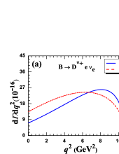
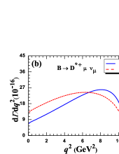
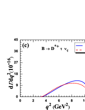
Figure 2: The $q^{\rm 2}$-dependence of $d\Gamma/dq^{\rm 2}$ for $B\to D^{*+}l^{-}\bar{\nu}_{\rm l}$ with $l=e,\mu,\tau$ in the pQCD approach (the solid curves), or in the HQET (the short-dashed curves). Here $q^{\rm 2}_{\rm max}$ = 10.69 GeV².

From the differential decay rates as given in Eqs.(19,24-26), it is easy to calculate the branching ratios for the considered decays by the integrations over $q^{\rm 2}$. We then find the pQCD predictions for the branching ratios of the eight $B\to D^{(*)}l^{-}\bar{\nu}_{\rm l}$ decays as listed in Table 2, where the individual theoretical errors have been added in quadrature. In order to check the relative size of the theoretical errors, we here present the pQCD predictions for ${\cal B}(B^{-}\to D^{0}\tau^{-}\bar{\nu}_{\rm\tau})$ and ${\cal B}(B^{-}\to D^{*0}\tau^{-}\bar{\nu}_{\rm\tau})$ with the individual errors:

$${\cal B}(B^{-}\to D^{0}\tau^{-}\bar{\nu}_{\rm\tau}) = \left[0.95^{+0.31}_{-0.25}(\omega_{\rm B})^{+0.19}_{-0.17}(f_{\rm B})\pm 0.04(V_{\rm cb})\pm 0.01(m_{\rm c})\right]\%,$$ (29)

$${\cal B}(B^{-}\to D^{*0}\tau^{-}\bar{\nu}_{\rm\tau}) = \left[1.47^{+0.29}_{-0.27}(\omega_{\rm B})^{+0.29}_{-0.27}(f_{\rm B})\pm 0.07(V_{\rm cb})\pm 0.10(m_{\rm c})\right]\%,$$ (30)

where the four major theoretical errors come from the uncertainties of the input parameters $\omega_{\rm B}=0.40\pm 0.04$ GeV, $f_{\rm B}=0.21\pm 0.02$ GeV, $|V_{\rm cb}|=(39.54\pm 0.89)\times 10^{-3}$ and $m_{\rm c}=1.35\pm 0.03$ GeV.

In Table 2, the pQCD predictions for the branching ratios of the eight decay modes are listed in column two. For the case of $l=(e,\mu)$, we list the averaged results. In column three, we show the HQET predictions obtained by direct calculations using the formulaes as given in Refs. prd85-094025 ; jhep2013-01054 The HQET predictions as given in Ref. prd85-094025 are listed in column four. The measured values as reported by BaBar prl109-101802 or quoted from PDG-2012 pdg2012 are also listed in last two columns as an comparison. One can see from the numerical results in Table 2 that

• The pQCD and HQET predictions for the branching ratios in fact agree with each other within one standard deviation, but the central values of the pQCD predictions for the branching ratios of the four $B\to D^{(*)}\tau\bar{\nu}_{\rm\tau}$ decays are a little larger than the HQET ones and show a better agreement with the measured values.

• Of course, the theoretical errors of the pQCD predictions are still large, say $\sim 35\%$. It is therefore necessary to define the ratios $R(X)$ among the branching ratios of the individual decays, since the theoretical errors are greatly canceled in these ratios.

Table 2: The theoretical predictions for ${\cal B}(B\to D^{(*)}l^{-}\bar{\nu}_{\rm l})$. The world averages from PDG 2012 pdg2012 and the measured values  prl109-101802 ; prd79-012002 ; prd77-032002 are also listed in last two columns.

Channels	pQCD(%)	HQET(%)	HQET(%)[5]	PDG(%)[34]	BaBar(%)
$\bar{B}^{0}\to D^{+}\tau^{-}\bar{\nu}_{\rm\tau}$	$0.87^{+0.34}_{-0.28}$	$0.63\pm 0.06$	$0.64\pm 0.05$	$1.1\pm 0.4$	$1.01\pm 0.22$
$\bar{B}^{0}\to D^{+}l^{-}\bar{\nu}_{\rm l}$	$2.03^{+0.92}_{-0.70}$	$2.13^{+0.19}_{-0.18}$	$-$	$2.18\pm 0.12$	$2.15\pm 0.08$
$B^{-}\to D^{0}\tau^{-}\bar{\nu}_{\rm\tau}$	$0.95^{+0.37}_{-0.31}$	$0.69\pm 0.06$	$0.66\pm 0.05$	$0.77\pm 0.25$	$0.99\pm 0.23$
$B^{-}\to D^{0}l^{-}\bar{\nu}_{\rm l}$	$2.19^{+0.99}_{-0.76}$	$2.30\pm 0.20$	$-$	$2.26\pm 0.11$	$2.34\pm 0.14$
$\bar{B}^{0}\to D^{*+}\tau^{-}\bar{\nu}_{\rm\tau}$	$1.36^{+0.38}_{-0.37}$	$1.25\pm 0.04$	$1.29\pm 0.06$	$1.5\pm 0.5$	$1.74\pm 0.23$
$\bar{B}^{0}\to D^{*+}l^{-}\bar{\nu}_{\rm l}$	$4.52^{+1.44}_{-1.31}$	$4.94\pm 0.15$	$-$	$4.95\pm 0.11$	$4.69\pm 0.34$
$B^{-}\to D^{*0}\tau^{-}\bar{\nu}_{\rm\tau}$	$1.47^{+0.43}_{-0.40}$	$1.35\pm 0.04$	$1.43\pm 0.05$	$2.04\pm 0.30$	$1.71\pm 0.21$
$B^{-}\to D^{*0}l^{-}\bar{\nu}_{\rm l}$	$4.87^{+1.60}_{-1.41}$	$5.35\pm 0.16$	$-$	$5.70\pm 0.19$	$5.40\pm 0.22$

4.3     The ratios of the branching ratios

Since the most hadronic and SM parameter uncertainties are greatly canceled in the ratios of the corresponding branching ratios, we firstly define the six R(X)-ratios in the same way as in Ref. prl109-101802 and compare our pQCD predictions with other theoretical predictions or the measured values. For the two isospin-constrained ratios $R(D)$ and $R(D^{*})$, for example, we find numerically

$$R(D) = 0.430^{+0.015}_{-0.022}(\omega_{\rm B})\pm 0.014(m_{\rm c}),$$ (31)

$$R(D^{*}) = 0.301^{+0.012}_{-0.013}(\omega_{\rm B})^{+0.005}_{-0.003}(m_{\rm c}),$$ (32)

where the major theoretical errors come from the uncertainties of $\omega_{\rm B}=0.40\pm 0.04$ GeV and $m_{\rm c}=1.35\pm 0.03$ GeV. The theoretical errors from the uncertainties of $f_{\rm B}$ and $|V_{\rm cb}|$ are canceled completely in the ratios of the branching ratios. It is easy to see that the theoretical errors of the pQCD predictions for R(X)-ratios are reduced significantly to about $5\%$.

Table 3: The theoretical predictions for the six R-ratios obtained by employing the pQCD approach or other theoretical methods, and the measured values prl109-101802 .

Ratio	pQCD	HQET	HQET [5]	SM [7,8]	SM [14]	SM [19]	BaBar [4]
$R(D^{0})$	$0.433^{+0.017}_{-0.027}$	$0.297^{+0.017}_{-0.016}$	$-$	$-$	$-$	$-$	$0.429\pm 0.097$
$R(D^{+})$	$0.428^{+0.023}_{-0.033}$	$0.297\pm 0.017$	$-$	$-$	$-$	$-$	$0.469\pm 0.099$
$R(D^{*0})$	$0.302^{+0.012}_{-0.014}$	$0.253\pm 0.004$	$-$	$-$	$-$	$-$	$0.322\pm 0.039$
$R(D^{*+})$	$0.301^{+0.012}_{-0.015}$	$0.252\pm 0.004$	$-$	$-$	$-$	$-$	$0.355\pm 0.044$
${\cal R}(D)$	$0.430^{+0.021}_{-0.026}$	$0.297\pm 0.017$	$0.296\pm 0.016$	$0.316$	$0.315$	$0.31$	$0.440\pm 0.072$
${\cal R}(D^{*})$	$0.301\pm 0.013$	$0.252\pm 0.004$	$0.252\pm 0.003$	$-$	$0.260$	$-$	$0.332\pm 0.030$

In Table 3, we list our pQCD predictions for all six R(X)-ratios in column two. As comparisons, we also show the HQET predictions obtained in this work or those as given in Refs. prd85-094025 , other SM predictions as presented in Refs. prl109-071802 ; prd85-114502 ; mpla27-1250183 ; Kosnik-1301 , and the measured values as reported by BaBar Collaboration prl109-101802 . From the numerical results as listed in Table II and III we find the following points:

• Due to the strong cancelation of the theoretical errors in the ratios of the corresponding branching ratios, the error of the pQCD predictions for all six R(X)-ratios are $\sim 5\%$ only, similar in size with the HQET ones (in this work or in Ref. prd85-094025 ) and other SM predictions prl109-071802 ; prd85-114502 ; mpla27-1250183 ; Kosnik-1301 .

• The SM predictions as given in Refs. prl109-071802 ; prd85-114502 ; mpla27-1250183 ; Kosnik-1301 are consistent with each other within their errors. One can see that, however, there still exist a clear discrepancy between these theoretical predictions for $R(D^{(*)})$ and the BaBar’s measurements prl109-101802 , although the gap become a little bit smaller than that in Ref. prd85-094025 .

• For $R(D)$ and $R(D^{*})$, the pQCD predictions agree very well with the data, the BaBar’s anomaly of $R(D^{(*)})$ are therefore explained successfully in the framework of the SM by employing the pQCD factorization approach.

• Besides $R(D^{(*)})$, the pQCD predictions for the central values of other four ratios $R(D^{0})$, $R(D^{+})$, $R(D^{*0})$ and $R(D^{*+})$ also agree very well with the corresponding BaBar measurements.

Analogous to above $R(D)$ and $R(D^{*})$ ratios, we can also define the new isospin-constrained ratios $R_{\rm D}^{l}$ and $R_{\rm D}^{\tau}$ in the form of

$$R_{\rm D}^{\rm l} \equiv \frac{{\cal B}(B\to D^{+}l^{-}\bar{\nu}_{\rm l})+{\cal B}(B\to D^{0}l^{-}\bar{\nu}_{\rm l})}{{\cal B}(B\to D^{*+}l^{-}\bar{\nu}_{\rm l})+{\cal B}(B\to D^{*0}l^{-}\bar{\nu}_{\rm l})},$$ (33)

$$R_{\rm D}^{\rm\tau} \equiv \frac{{\cal B}(B\to D^{+}\tau^{-}\bar{\nu}_{\rm\tau})+{\cal B}(B\to D^{0}\tau^{-}\bar{\nu}_{\rm\tau})}{{\cal B}(B\to D^{*+}\tau^{-}\bar{\nu}_{\rm\tau})+{\cal B}(B\to D^{*0}\tau^{-}\bar{\nu}_{\rm\tau})}.$$ (34)

In the ratio $R(D)$ ( $R(D^{*})$), the involved decays have the same final state meson $D$ ( $D^{*}$), but different leptons. The value of the ratio $R(D^{(*)})$ dominantly depend on the mass difference between large $m_{\rm\tau}$ and tiny $m_{\rm l}$ with $l=(e,\mu)$. For the two new ratios $R_{\rm D}^{\rm l}$ and $R_{\rm D}^{\rm\tau}$, however, the relevant decays appeared in one ratio have the same final state leptons but different final state mesons: $D$ in the numerator and $D^{*}$ in the denominator. The new ratio $R_{\rm D}^{\rm l}$ and $R_{\rm D}^{\rm\tau}$ will measure the effects induced by the variations of the form factors for $B\to D$ and $B\to D^{*}$ transition, respectively. In other words, the new ratios $R_{\rm D}^{l}$ and $R_{\rm D}^{\tau}$ may be more sensitive to the QCD dynamics which controls the $B\to D^{(*)}$ transitions than the “old” ratios $R(D)$ and $R(D^{*})$. We therefore suggest the experimental measurements for the new ratios $R_{\rm D}^{\rm l}$ and $R_{\rm D}^{\rm\tau}$ as soon as possible.

Following the same procedure as for $R(D^{(*)})$ ratios, it is straight forward to find the pQCD predictions for the new $R_{\rm D}^{\rm l,\tau}$ numerically: $R_{\rm D}^{\rm l}=0.450^{+0.064}_{-0.051}$ and $R_{\rm D}^{\rm\tau}=0.642^{+0.081}_{-0.070}$, here the dominant errors come from the uncertainty of $\omega_{\rm B}=0.40\pm 0.04$ GeV and $m_{\rm c}=1.35\pm 0.03$ GeV. The error of the pQCD predictions for ratio $R_{\rm D}^{\rm l}$ and $R_{\rm D}^{\rm\tau}$ is about $15\%$.

5. Summary

In summary, we studied the semileptonic decays $B\to D^{(*)}l^{-}\bar{\nu}_{\rm l}$ in the framework of the SM by employing the pQCD factorization approach. From the numerical calculations and phenomenological analysis we found that

• The pQCD predictions for the branching ratios ${\cal B}(B\to D^{(*)}l^{-}\bar{\nu}_{\rm l})$ agree well with other SM predictions and the measured values within one standard deviation.

• For the isospin-constrained ratios $R(D)$ and $R(D^{*})$, the pQCD predictions are

  $$R(D)=0.430^{+0.021}_{-0.026},\quad R(D^{*})=0.301\pm 0.013.$$ (35)

  We therefore provide a SM interpretation for the BaBar’s $R(D^{(*)})$ anomaly.

• For the newly defined ratios $R_{\rm D}^{\rm l,\tau}$, the pQCD predictions are

  $$R_{\rm D}^{\rm l}=0.450^{+0.064}_{-0.051},\quad R_{\rm D}^{\rm\tau}=0.642^{+0.081}_{-0.070},$$ (36)

  These new ratios may be more sensitive to the QCD dynamics of the considered decays than the ratios $R(D^{(*)})$, we therefore suggest the experimental measurements for them in the forthcoming experiments.

References

• (1) Aubert B et al BABAR Collaboration (2008) Observation of semileptonic decays $B\to D^{*}\tau^{-}\bar{\nu}_{\rm\tau}$ and Evidence for $B\to D\tau^{-}\bar{\nu}_{\rm\tau}$. Phys Rev Lett. 100(02): 021801
• (2) Matyja A et al Belle Collaboration (2007) Observation of $B^{0}\to D^{*-}\tau^{+}\nu_{\rm\tau}$ Decay at Belle. Phys Rev Lett. 99(19): 191807
• (3) Bozek A et al Belle Collaboration (2010) Observation of $B^{+}\to\bar{D}^{*0}\tau^{+}\nu_{\rm\tau}$ and Evidence for $B^{+}\to\bar{D}^{*0}\tau^{+}\nu_{\rm\tau}$ at Belle. Phys Rev D 82(07): 072005
• (4) Lees J P et al BABAR Collaboration (2012) Evidence for an Excess of $\bar{B}\to D^{(*)}\tau\bar{\nu}_{\rm\tau}$ Decays. Phys Rev Lett. 109(10): 101802
• (5) Fajfer S, Kamenik J F, Nisandzic I (2012) On the $B\to D^{*}\tau\bar{\nu}_{\rm\tau}$ Sensitivity to New Physics. Phys Rev D 85(09): 094025
• (6) Bozek A (for Belle Collaboration) (2013) The $B\to\tau\nu$ and $B\to\bar{D}^{(*)}\tau^{+}\bar{\nu}_{\rm\tau}$ measurements. talk given at FPCP 2013, May 3-6, 2013, Buzios, Breizl
• (7) Bailey J A et al (2012) Refining new-physics searches in $B\to D\tau\nu$ decay with lattice QCD. Phys Rev Lett. 109(07): 071802
• (8) Bailey J A et al Fermilab Lattice and MILC Collaborations (2012) $B_{\rm s}\to D_{\rm s}/B\to D$ semileptonic form-factor ratios and their application to $BR(B^{\rm 0}_{\rm s}\to\mu^{+}\mu^{-}$. Phys Rev D 85(11):114502; Errotem 86(03): 039904
• (9) Fajfer S, Kamenik J F, Nisandzic I et al (2012) Implications of Lepton Flavor Universality Violations in B Decays. Phys Rev Lett. 109(16):161801
• (10) Crivellin A, Greub C, Kokulu A (2012) Explaining $B\to D\tau\nu,B\to D^{*}\tau\nu$ and $B\to\tau\nu$ in a 2HDM of type III. Phys Rev D 86(05):054014
• (11) Celis A, Jung M, Li X Q et al (2013) Sensitivity to charged scalars in $B\to D\tau\nu$ and $B\to\tau\nu$ decays. JHEP 2013(01): 054
• (12) Datta A, Duraisamy M, Ghosh D (2012) Diagnosing new physics in $b\to c\tau\nu$ decays in the light of the recent BABAR result. Phys Rev D 86(03): 034027
• (13) Choudhury D, Ghosh D K, Kundu A (2012) B decay anomalies in an effective theory. Phys Rev D 86(11):114037
• (14) Faustov R N, Galkin V O (2012) Exclusive weak B decays involving $\tau$ lepton in the relativistic quark model. Mod Phys Lett A 27(31): 1250183.
• (15) Fajfer S and Nisandzic I (2013) Theory of $B\to\tau\nu$ and $B\to D^{*}\tau\nu$. Conference: C12-09-28; arXiv:1301.1167 [hep-ph]
• (16) Pich A (2013) TAU2012 Summary. summary talk given at TAU 2012, 17-21 Sep. 2012, Nagoya, Japan; arXiv:1301.4474 [hep-ph]
• (17) Ricciardi G (2012) Semileptonic B decays. Conference: C12-10-08.1, PoS ConfinementX, 2012:145
• (18) Stone S (2013) New physics from flavour. Conference: C12-07-04, PoS ICHEP2012 2013:033
• (19) Becirevic D, Kosnik N, Tayduganov A (2012) $\bar{B}\to D\tau\bar{\nu}_{\rm\tau}$ vs. $\bar{B}\to D\mu\bar{\nu}_{\mu}$. Phys Lett B 716: 208-213
• (20) Aubert B et al BaBar Collaboration (2010) Measurement of $V_{cb}$ and the Form-Factor Slope in $B\to Dl\nu$ Decays in Events Tagged by a Fully Reconstructed B Meson. Phys Rev Lett. 104(01): 011802
• (21) Wang W F, Xiao Z J (2012) Semileptonic decays $B/B_{\rm s}\to(\pi,K)(l^{+}l^{-},l\nu,\nu\bar{\nu})$ in the perturbative QCD approach beyond the leading order. Phys Rev D 86(11):114025
• (22) Wang W F, Fan Y Y, Liu M, Xiao Z J (2013) Semileptonic decays $B_{\rm s}\to(\eta,\eta^{(\prime)},G)(l^{+}l^{-},l\nu,\nu\bar{\nu})$ in the perturbative QCD approach beyond the leading order. Phys Rev D 87(09): 097501
• (23) Li H N (2003) QCD Aspects of Exclusive B Meson Decays. Prog.Part. $\&$ Nucl. Phys. 51:85-171
• (24) Li H N (1995) Applicability of perturbative QCD to $B\to D$ decays. Phys Rev D 52:3958-3965.
• (25) Kurimoto T, Li H N, Sanda A I (2003) $B\to D^{(*)}$ form factors in perturbative QCD. Phys Rev D 67(05):054028
• (26) Xiao Z J, Wang W F, Fan Y Y (2012) Revisiting the pure annihilation decays $B_{s}\to\pi^{+}\pi^{-}$ and $B^{0}\to K^{+}K^{-}$: The data and the perturbative QCD predictions. Phys Rev D 85(09): 094003
• (27) Fan Y Y, Wang W F, Cheng S, Xiao Z J (2013) Anatomy of $B\to K\eta^{(^{\prime})}$ decays in different mixing schemes and effects of next-to-leading order contributions in the perturbative QCD approach. Phys Rev D 87(09):094003
• (28) Liu X, Li H N, Xiao Z J (2012) Implications on $\eta-\eta^{\prime}$-glueball mixing from $B_{d,s}\to J/\psi\eta^{(^{\prime})}$ decays. Phys Rev D 86(01): 011501(R)
• (29) Li R H, LΓΌ C D, Zou H (2008) $B(B_{s})\to D_{(s)}P,D_{s}V,D^{*}_{(s)}P,D^{*}_{s}V$ decays in the pQCD approach. Phys Rev D 78(01): 014018
• (30) Kurimoto T, Li H N, Sanda A I (2001) Leading power contribution to $B\to\pi\rho$ transition form factors. Phys Rev D 65(01): 014007
• (31) Lu C D, Ukai K, Yang M Z (2001) Branching ratio and CP violation of $B\to\pi\pi$ decays in the perturbative QCD approac. Phys Rev D 63(07): 074009
• (32) Li R H, LΓΌ C D, Wang W et al (2009) $B\to S$ transition form factors in the perturbative QCD approach. Phys Rev D 79(01): 014013
• (33) Wang W, Shen Y L, LΓΌ C D (2009) Covariant light-front approach for $B_{c}$ transition form factors. Phys Rev D 79(05): 054012
• (34) Particle Data Group, Beringer J et al (2012) Phys Rev D 86(01):010001
• (35) Heavy Flavor Averaging Group, Amhis Y et al (2012) Averages of b-hadron, c-hadron, and tau-lepton properties as of early 2012, arXiv:1207.1158 [hep-ex]; and online update at http://www.slac.stanford.edu/xorg/hfag
• (36) Keum Y Y, Li H N, Sanda A I (2001) Fat penguins and imaginary penguins in perturbative QCD. Phys Lett B 504:6-14
• (37) Keum Y Y, Li H N, Sanda A I (2001) Penguin enhancement and $B\to K\pi$ decays in perturbative QCD. Phys Rev D 63(05): 054008
• (38) Cheng H Y, Chua C K, Hwang C W (2004) Covariant light-front approach for s-wave and p-wave mesons: its application to decay constants and form factors. Phys Rev D 69(07): 074025
• (39) Falk A F, Neubert M (1993) Second order power corrections in the heavy quark effective theory. 1. Formalism and meson form-factors. Phys Rev D 47:2965-2981
• (40) Falk A F, Neubert M (1993) Second order power corrections in the heavy quark effective theory. 2. Baryon form-factors. Phys Rev D 47:2982-2990
• (41) Neubert M (1992) Short distance expansion of heavy quark currents. Phys Rev D 46:2212-2227
• (42) Neubert M (1994) Heavy quark symmetry. Phys Rept 245:259-396
• (43) Grozin A (2004) Heavy Quark Effective Theory, Springer, STMP 201
• (44) I.Β Caprini, L.Β Lellouch and M.Β Neubert (198) Dispersive bounds on the shape of $\bar{B}\to D^{(*)}l\bar{\nu}_{\rm l}$ form-factors. Nucl Phys B 530:153-181
• (45) Aubert B et al BABAR Collaboration (2009) Measurements of the semileptonic decays $B\to Dl\nu$ and $B\to D^{*}l\nu$ using a global fit to $DXl\nu$ final states. Phys Rev D 79(01): 012002
• (46) Aubert B et al BABAR Collaboration (2008) Determination of the form factors for the decay $B^{0}\to D^{*-}l\nu$ and of the CKM matrix element $V_{\rm cb}$. Phys Rev D 77(03): 032002