Hydrodynamic and field-theoretic approaches of light localization in open media

Abstract

Many complex systems exhibit hydrodynamic (or macroscopic) behavior at large scales characterized by few variables such as the particle number density, temperature and pressure obeying a set of hydrodynamic (or macroscopic) equations. Does the hydrodynamic description exist also for waves in complex open media? This is a long-standing fundamental problem in studies on wave localization. Practically, if it does exist, owing to its simplicity macroscopic equations can be mastered far more easily than sophisticated microscopic theories of wave localization especially for experimentalists. The purposes of the present paper are two-fold. On the one hand, it is devoted to a review of substantial recent progress in this subject. We show that in random open media the wave energy density obeys a highly unconventional macroscopic diffusion equation at scales much larger than the elastic mean free path. The diffusion coefficient is inhomogeneous in space; most strikingly, as a function of the distance to the interface, it displays novel single parameter scaling which captures the impact of rare high-transmission states that dominate long-time transport of localized waves. We review aspects of this novel macroscopic diffusive phenomenon. On the other hand, it is devoted to a review of the supersymmetric field theory of light localization in open media. In particular, we review its application in establishing a microscopic theory of the aforementioned unconventional diffusive phenomenon.

I Introduction and motivation

Anderson localization is one of the most profound concepts in modern condensed matter physics (see Refs. Abrahams10 and Mirlin08 for recent reviews). While this phenomenon was originally predicted for electron systems Anderson58 , direct observations of electron wave localization are notably difficult because of electron-electron interactions. In the eighties, the universality of Anderson localization as a wave phenomenon was appreciated by many researchers John83a ; John83 ; John84 ; John85 ; Anderson84 . The study of classical wave localization is now a flourishing field Sheng90 ; Sheng95 ; Lagendijk09 . In recent years the unprecedented level reached in manipulating dielectric materials Wiersma97 ; Wiersma99 ; Maret97 ; Genack00 ; Fishman07 ; Wiersma08 ; Genack06 ; Maret06 ; Maret07 ; Zhang09 ; Zhang10 and elastic media Weaver98 ; Hu09 has led to substantial experimental progress in studies of Anderson localization in various classical wave systems. Together with the realization of Anderson localization in ultracold atomic gases Billy08 ; Roati08 , these experiments have raised many fundamental issues, and are triggering a renewal of localization studies. In addition, the experimental observation of Cao and co-workers Cao02 has triggered considerable investigations of using Anderson localization of light for random lasing (see Ref. Wiersma08a for a review).

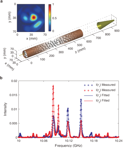
Figure 1: Example of light transport through open media. Upper panel: microwave radiation is launched from a horn placed before the sample, a copper tube consisting of randomly positioned alumina spheres. Wave intensity on the output plane is measured by the detector placed in front of the sample. Lower panel: intensity spectra at different positions ${\bf r}_{1,2}$ of the output plane. (Adapted by permission from Macmillan Publishers Ltd: Nature 471, 345-348, $\copyright$ 2011)

Since photons do not mutually interact, it was anticipated Anderson84 ; John84 ; John87 that classical electromagnetic waves may serve as an ideal system for experimental studies of Anderson localization. Ground-breaking experimental achievement was made in 2000 when unambiguous evidence of microwave localization in quasi one-dimensional (Q$1$D) samples was observed Genack00 . Since then substantial experimental progress in electromagnetic wave localization have been achieved. Among them are dynamics of localized microwave radiation in Q$1$D samples Zhang09 ; Zhang10 , time-resolved transmission of light through slab media Maret06 ; Maret07 , measurements of the spatial distribution of the localized modes Sebbah06 , and the observation of two-dimensional Anderson localization in photonic lattices Fishman07 . It has also been within the reach of microwave experiments on Q$1$D localized samples the statistics of quasi-normal modes Genack11 and transmission eigenvalues Genack12 . In particular, the crystallization of transmission eigenvalue distribution Dorokhov82 ; Mello88 ; Frahm95 ; Rejaei96 ; Zirnbauer04 ; Tian05 , has been observed recently. While these experimental studies have not yet been carried out in other wave systems, they further show that classical electromagnetic waves have great advantages in experimental studies of localization.

Importantly, experimental setups for probing localization of electromagnetic waves Maret06 ; Genack00 ; Zhang09 ; Zhang10 ; Zhang03 ; Zhang04 ; Lagendijk97 ; Maret99 and other classical waves Hu09 typically are very different from those for quantum matter waves Billy08 ; Roati08 . In the former, wave energies leak out of random media through interfaces and measurements are performed outside media. Specifically, in transmission experiments, waves are launched into the system on one side and detected on the other (Fig. 1); in coherent backscattering experiments (see Ref. Maret09 for a review), the light beam is launched into and exit from the medium at the same air-medium interface, and the angular variation of the reflected intensity is measured (Fig. 2). Theoretically, one treats the former system as a finite-sized open medium and the latter one (often) as a semi-infinite open medium. Therefore, these classical wave experiments address a fundamental issue – the localization property of open systems – which, as we will see throughout this review, conceptually differs from that of bulk (infinite) systems.

In fact, open systems have been at the core of localization studies for several decades. In the mid-seventies, Thouless and co-workers noted that the unique parameter governing the evolution of eigenstates when the system’s size is scaled is the dimensionless conductance (which is nowadays called the Thouless conductance), a main transport characteristic of open (electronic) systems Thouless74 . This eventually led to the advent of the milestone discovery – the single parameter scaling theory of Anderson localization – in 1979 Anderson79 . Shortly later, Anderson and co-workers further pointed out Anderson80 that since the resistance displays a broad distribution in the (one-dimensional) strongly localized regime, it is not sufficient to study the scaling behavior of the average conductance. Instead, one must study how the entire conductance distribution evolves as the sample size increases. In fact, long before the Anderson localization theory was developed, such a distribution was discovered by Gertsenshtein and Vasil’ev in a study of the exponential decay of radio waves transporting through waveguides with random inhomogeneities. Importantly, the large-conductance tail of the distribution represents rare localized states peaked near the sample center with exponentially long lifetime Lifshits79 ; Azbel83 ; Azbel83a ; Freilikher03 . These states have been found experimentally to be responsible for long-time transport of localized waves through open systems Zhang09 . They have high transmission values that may be close to unity, in sharp contrast to typical localized states with exponentially small transmission. Such peculiar features are intrinsic to open medium. The high transmission states even promise to have practical applications: they mimic a ‘resonator’ with high-quality factors (due to the long lifetime) in optics and thus can be used to fabricate a random laser Milner05 . In combination with optical nonlinearity, it can also be used to realize optical bistability Freilikher10 .

Nowadays experimental and theoretical results on global transport properties (in the sense of that they provide no information on wave propagation inside the medium) – characterized by conductance, reflection, transmission, etc. – of both classical and de Broglie waves in one-dimensional open media have been well documented (for a review, see, e.g., Ref. Mirlin00 ). An essential difference between finite-sized open system and infinite (closed) system was pointed out by Pnini and Shapiro Shapiro96 . That is, the wave field is a sum of traveling waves for the former and of standing waves for the latter. Let us mention a few more recent results in order for readers to better appreciate the rich physics arising from the interplay between localization and openness of the medium. In Ref. Genack06 , it was found that, surprisingly, even low absorptions essentially improve the conditions for the detection of disordered-induced resonances in reflection as compared with the absorptionless case. In Ref. Fyodorov03 , Fyodorov considered reflection of waves injected into a disordered medium via a single channel waveguide, and discovered the spontaneous breakdown of $S$-matrix unitarity. Interestingly, this may serve as a new signature of Anderson transition in high dimension. Much less is known regarding how wave propagates inside the medium. Nevertheless, they may provide a key to many new experimental results such as the spatial distribution of localized modes Sebbah06 and the interplay between absorption (gain) and resonant states Genack06 .

In principle, one may describe the wave field in terms of the superposition of quasi-normal modes Zhang09 ; Genack11 ; Ching98 namely the eigenmodes of the Maxwell equation in the presence of open boundary. This exact approach carries full information on wave propagation but in general must be implemented by experiments or numerical simulations. As we are interested in physics at scales much larger than the elastic mean free path, alternative yet simpler approach might exist. The situation might be similar to that of many complex systems like fluids. There, many degrees of freedom causing the complexity of dynamics notwithstanding, at macroscopic scales (much larger than the mean free path) the system’s physics is well described by few variables such as the particle number density, temperature and pressure and a set of hydrodynamic (or macroscopic) equations. In fact, for open diffusive media, such a macroscopic equation is well known which is the normal diffusion equation of wave energy density reflecting Brownian motion of classical photons. For open localized media, the normal diffusion equation breaks down. The question of fundamental interests and practical importance – addressed from experimental viewpoints by many researchers for decades Lagendijk00 ; Skipetrov04 ; Skipetrov06 ; Zhang09 ; Weaver98 ; Maret09 – thereby arises: is the macroscopic description valid for open localized media? Since the eighties Berkovits87 ; Edrei90 ; Berkovitz90a there have been substantial efforts in searching for a generalized macroscopic diffusive model capable of describing propagation of localized waves in open media. In the past decade, research activity in this subject has intensified Zhang09 ; Hu09 ; Lagendijk00 ; Skipetrov04 ; Skipetrov06 ; Tian08 ; Skipetrov08 ; Tian10 ; Skipetrov10 . In essence, one looks for certain generalization of Fick’s law with the detailed knowledge of multiple wave scattering entering into the generalized diffusion coefficient. Such a diffusive model has the advantage of technical simplicity over many sophisticated first-principles approaches, and may provide a simple principle for guiding experimental studies (see Ref. Maret09 for a review).

Important progress was achieved by van Tiggelen and co-workers in 2000 Lagendijk00 . These authors noticed that in open media weak localization effects of waves are inhomogeneous in space. Therefore, they hypothesized the position dependence of the one-loop weak localization correction to the diffusion coefficient. By further introducing a key assumption – the validity of the one-loop self-consistency, they obtained a phenomenological, nonlinear macroscopic diffusion model describing static transport of localized waves in open media. Later, the proposed self-consistent local diffusion (SCLD) model was extended to the dynamic case Skipetrov04 ; Skipetrov06 . In the past decade the SCLD model has been used to guide considerable research activities in classical wave localization. The subjects include: static reflection and transmission of light in systems near the mobility edge Lagendijk00 , dynamic reflection and transmission of Q$1$D weakly localized waves Skipetrov04 , dynamics of Anderson localization in three-dimensional media Skipetrov06 , transmission of localized acoustic waves through strongly scattering plates Hu09 , and transmission and energy storage in random media with gain Yamilov10 .

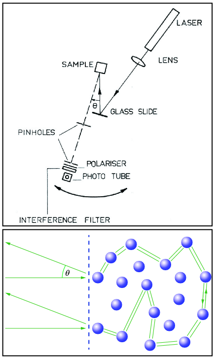
Figure 2: Example of light transport through open media. Experimental setup (upper panel) of coherent backscattering (lower panel): a beam of light is launched into and backscattered by a semi-infinite random medium. (upper panel: from Ref. Maret85 with reproduction permission from G. Maret $\copyright$ The American Physical Society)

This prevailing model was first examined in Ref. Zhang09 in experiments on pulsed microwave transmission in Q$1$D localized samples. The SCLD model failed to describe the experimental results. In fact, in these systems, the long-time transport of localized waves is determined by rare disorder-induced resonant transmissions. In addition, the SCLD model fails to describe results obtained from numerical simulations on static (long-time limit) wave transport through one-dimensional localized samples Tian10 ; Skipetrov10 . Since the macroscopic diffusive model describes local (in space) behavior of wave propagation (in the average sense), it is very ‘unlikely’ that it could capture simultaneously two prominent features of resonant transmissions. That is, they are rare events and objects highly non-local in space. In fact, it had been commonly suspected that eventually the validity of the macroscopic diffusion concept in open systems would be washed out by these rare events. On the other hand, the predictions of the SCLD model agree with the experimental results in higher dimensions Hu09 . In view of these contradictory observations one inevitably has to re-examine the fundamental issue: whether and how do localized waves in open media exhibit macroscopic diffusion?

A preliminary but very surprising answer to this question was provided in a first-principles study of static transport of localized waves in one-dimensional open media Tian10 . It turns out that in these systems, the macroscopic diffusion (or equivalently Fick’s law) concept never breaks down at scales much larger than the elastic mean free path. Rather, in depending on the distance to the interface, the diffusion coefficient exhibits novel scaling. It is such scaling that unifies the objects of resonant transmission and macroscopic diffusion. The novel scaling behavior is missed by the phenomenological SCLD model. In this review, we will discuss the existence of such highly unconventional macroscopic diffusion in more general situations (e.g., dynamic transport and in high dimensions). It is believed that waves propagating through open media may exhibit even richer macroscopic behavior. As such, the unconventional macroscopic diffusion of waves in open media may potentially open a new direction for the study of Anderson localization. One of the main purposes of this paper is to review various aspects of this diffusion phenomenon such as its microscopic mechanism, microscopic theory and perspectives.

Technically, treatments of localization in open media differ dramatically from those of infinite media. The study of open systems has proved to be an extremely difficult task especially for high dimensions and in the dynamic case. Recall that for infinite electron systems, the diagrammatic technique Woelfle80a ; Woelfle80 ; Woelfle92 ; Woelfle10 ; Larkin79 has had considerable successes in (approximate) studies of a variety of localization phenomena, e.g., one-loop weak localization, strong localization, and criticality of Anderson transition (see Refs. Woelfle92 ; Woelfle10 for reviews). In view of these successes, it is natural to extend this technique to classical wave systems, and this has been done by many authors Kroha93 ; Nieh98 ; Kirkpatrick85 . In the past, the non-perturbative diagrammatic theory of Vollhardt and Wölfle (VW) Woelfle80a ; Woelfle80 , having the advantage of technical simplicity, has become a popular approach in studies of classical wave localization. Furthermore, it has been noticed Suslov12 ; Lagendijk00 ; Skipetrov04 ; Skipetrov06 ; Skipetrov08 that it is possible to generalize the VW theory appropriately to describe transport of strongly localized waves in open media. It should be emphasized that the rational of the original VW theory Woelfle80a ; Woelfle80 is built upon the exact Ward identity Woelfle80 ; Nieh98 ; Nieh98a and the sophisticate summation over the dominant infrared divergent diagrams (see Refs. Woelfle92 ; Suslov07 for a technical review). This rational is at the root of the one-loop self-consistency and to the best of my knowledge, has not yet been established for open media. These considerations necessitate the invention of an exact theory beyond simple one-loop perturbation.

There have been few attempts John83a ; John84 ; John83 ; John85 ; Lai12 of generalizing the replica field theory Wegner79 ; Wegner80 ; Efetov80 and the Keldysh field theory Kamenev10 to classical wave systems. However, these studies John83a ; John84 ; John83 ; John85 ; Lai12 focus on infinite random media. For open systems some exact solutions for Q$1$D strong localization have been found by using the replica field theory Tian05 . As for the replica field theory, in general, its applicability in the strongly localized regime needs further investigations due to the well-known problem of analytic continuation Efetov97 ; Zirnbauer84 . As for the Keldysh field theory, it does not encounter such a difficulty. However, to the best of my knowledge, it is not clear how to use this theory to obtain concrete results for strong localization. Finally, the Dorokhov-Mello-Pereyra-Kumar (DMPK) equation Beenakker97 ; Dorokhov82 ; Mello88 is an exact theory and a very powerful approach to Q$1$D strong localization in open media. The special case of the DMPK equation in one dimension was discovered as early as in 1959 Vasilev59 . But, it mainly provides information on global transport properties such as transmission and its fluctuations; it provides no information on local wave transport properties: it could not describe how waves propagate from one point to the other inside media. For example, by using this theory one could not judge the possibility of generalizing Fick’s law to localized open media. In addition, it is well-known that the DMPK equation is valid only in one dimension.

The supersymmetric approach escapes all these key difficulties. In Ref. Chernyak92 , the supersymmetric quantum mechanics was used to study reflection of classical waves by one-dimensional semi-infinite disordered medium. The supersymmetric field theory invented by Efetov Efetov82b ; Efetov83 ; Efetov97 was used by Mirlin and co-workers to study the deviation from the Rayleigh distribution of classical light intensity in diffusive Q$1$D samples (see Ref. Mirlin00 for a review). In Ref. Tian08 , the supersymmetric field theory was generalized to high-dimensional open media with internal reflection, and was employed to investigate dynamic transport of classical waves in high-dimensional open media. In particular, the unconventional macroscopic diffusion was discovered in Ref. Tian10 from this first-principles theory Tian08 . In fact, the machinery of supersymmetric field theory has become a standard approach in studies of disordered electronic systems. Nonetheless, researchers working on classical wave localization are less familiar with this technique. On the other hand, there are a number of recently observed phenomena regarding classical wave transport through open media which can be thoroughly studied by using this technique. These include effects of internal reflection on transmission fluctuations Genack12 and dynamics of localized waves Zhang09 . Since there are many prominent differences between classical and electronic waves (e.g., the condition of strong localization John83a ; John84 ), and a review of the application of the supersymmetric field theory in light localization has been absent, it is necessary to introduce here this technique – in the context of transport of classical electromagnetic waves through open random media – at a pedagogical level, which serves another main topic of this review.

The review is written in a self-contained manner, with the hope that readers wishing to master the supersymmetric technique and then apply it to classical wave systems could follow most technical details without resorting to further technical papers. Because of this, it could not be a complete introduction of this advanced theory. In fact, there have been a comprehensive book Efetov97 and several excellent reviews Efetov83 ; Mirlin00 ; Mirlin00a ; Mirlin08 covering various aspects of supersymmetric field theory. In particular, we will not introduce non-perturbative treatments Zirnbauer04 ; Efetov83a ; Zirnbauer91 ; Hueffmann90 ; Zirnbauer92 ; Zirnbauer94 , because these are technically highly demanding. The present review, implemented with substantial technical details, may be considered as a ‘first course in practicing the supersymmetric field theory’. It aims at helping the researchers working in the field of classical wave localization to become familiar with formulating large-scale wave dynamics in terms of supersymmetric functional integral formalism and further to master its perturbative treatments. With these preparations, readers may be ready to manipulate its non-perturbative treatments after further resorting to original technical papers and reviews. We emphasize that although the present review is written in the context of classical waves, unconventional macroscopic diffusion to be reviewed below is a universal wave phenomenon in open systems. In particular, it also exists for de Broglie waves.

For simplicity, we shall focus on scalar waves throughout this review. We shall not distinguish the concepts of (classical) scalar wave, electromagnetic wave, and light. The remainder of this review is organized as follows. In Sec. II we will review a number of research activities in studies of transport of localized waves through open media. These studies may be roughly classified into two categories: one is based on the macroscopic diffusion picture and the other on the mode picture. In Sec. III we will discuss in a heuristic manner the ‘origin’ of supersymmetry in studies of disordered systems. In Sec. IV we will proceed to introduce the supersymmetric field theory suitable for calculating various physical observables in random open media. Then, in Sec. V, we will apply this theory to study a special quantity, the spatial correlation of wave intensity. In particular, we will develop a general theory of unconventional macroscopic diffusion for the general case of a random slab. In Sec. VI, we will study in details the special case of one-dimensional unconventional macroscopic diffusion. In particular, we will present the explicit results for the static local diffusion coefficient and provide corroborating numerical evidence. Finally, we conclude in Sec. VII. In order to make this review self-contained, we include a number of technical details in Appendices A-E.

II Macroscopic diffusion versus mode picture of wave propagation

In infinite three (or higher)-dimensional systems, the envelope of eigenfunctions decays exponentially in space for the distance from the center far exceeding the localization length, $\xi$, when disorder is strong. Below or in two dimensions, even weak disorders lead to localization Abrikosov79 ; Berezinskii79 ; Berezinskii73 ; Efetov83a ; Mott61 ; Anderson79 . The (asymptotic) exponential decay of eigenfunctions in space is a key characteristic of localized waves in the mode picture. Can localized waves be understood in terms of the macroscopic diffusion picture? Recall that in the absence of wave interference effects, light exhibits pure ‘particle (classical photons)’ behavior, which in random environments is the well-known Brownian motion (We shall not consider here the case where the motion of photons is non-Brownian.) or normal diffusion of photons. When wave interference is switched on, localization effects set in. It has been well established that the latter does not render the macroscopic diffusion concept invalid Abrikosov79 ; Berezinskii79 ; Efetov83a ; Efetov83 ; Woelfle80a ; Woelfle80 ; Woelfle92 ; Woelfle10 ; Hikami81 . Rather, they (strongly) renormalize the Boltzmann diffusion constant. Specifically, given the point like source $J_{t}({\bf r}^{\prime})$ located at ${\bf r}^{\prime}$, the disorder averaged intensity profile at time $t$ is given by Chernyak92 $I({\bf r},t)=\int\frac{d\omega}{2\pi}\frac{d\tilde{\omega}}{2\pi}e^{i\tilde{\omega}t}{\cal Y}({\bf r},{\bf r}^{\prime};\tilde{\omega})J_{\omega+\frac{\tilde{\omega}}{2}}({\bf r}^{\prime})J_{\omega-\frac{\tilde{\omega}}{2}}^{*}({\bf r}^{\prime})$, where $J_{\omega}({\bf r}^{\prime})$ is the spectral decomposition of the source. Here, we have introduced the spatial correlation function defined as

$${\cal Y}({\bf r},{\bf r}^{\prime};\tilde{\omega})\equiv\left\langle G^{A}_{(\omega+\frac{\tilde{\omega}^{+}}{2})^{2}}({\bf r},{\bf r}^{\prime})\,G^{R}_{(\omega-\frac{\tilde{\omega}^{+}}{2})^{2}}({\bf r}^{\prime},{\bf r})\right\rangle$$ (1)

in the frequency domain. Here, $G^{R,A}_{(\omega\mp\frac{\tilde{\omega}^{+}}{2})^{2}}$ are the retarded (advanced) Green functions whose explicit definitions will be given in Sec. III.1. Throughout this review we use $\langle\cdot\rangle$ to denote the disorder average. Most importantly, the correlation function satisfies Woelfle92 ; Efetov97

$$(-i{\tilde{\omega}}-D({\tilde{\omega}})\nabla^{2}){\cal Y}({\bf r},{\bf r}^{\prime};{\tilde{\omega}})=\delta({\bf r}-{\bf r}^{\prime}).$$ (2)

It is important that here, the diffusion coefficient, $D({\tilde{\omega}})$, is frequency-dependent. The latter accounts for the retarded nature of the response to the spatial inhomogeneity of the wave energy density.

How are the mode and macroscopic diffusion pictures modified in open media? For the mode picture, because of the energy leakage through the system’s boundary, the Hermitian property is destroyed. Consequently, one describes transport in terms of quasi-normal modes Genack11 ; Zhang09 ; Ching98 each of which has a finite lifetime. Loosely speaking, wave energy is pumped into these modes, stored there and emitted in the course of time. For the macroscopic diffusion picture, substantial conceptual issues arise. In this section, we will review great efforts made in extending the macroscopic diffusion concept to localized wave transport through open media.

II.1 Electromagnetic wave propagation: macroscopic diffusion picture

Macroscopic diffusive approach to light transport may be dated back to the first half of last century, when the Boltzmann-type kinetic equation was used to study radiation transfer in certain astrophysical processes Chandrasekhar . In fact, it is a canonical procedure of deriving a normal diffusion equation – valid on the scale much larger than the transport mean free path, $l$ – from the Boltzmann kinetic equation. In the normal diffusion equation, the diffusion constant $D(\tilde{\omega})=cl/d\equiv D_{0}$, where $d$ is the dimension and $c$ the wave velocity. Notice that the latter may be reduced by the scattering resonance Niuwenhuizen which we shall not further discuss, and from now on we set $c$ to unity.

The Boltzmann transport theory essentially treats light scattering off dielectric fluctuations as Brownian motion of classical particles, the ‘photons’, and ignore the wave nature of light. However, the latter gives rise to interference effects which have far-reaching consequences. A canonical example is the coherent backscattering of light from semi-infinite diffusive media (Fig. 2, lower panel). There, two photon paths following Brownian motion may counterpropagate and thus constructively interfere with each other Altshuler83 ; Bergmann84 , leading to enhanced backscattering Maret09 ; Golubentsev84 ; Lagendijk85 ; Maret85 ; Akkermans86 . Effects of wave interference are even more pronounced in low dimensions ($d\leq 2$) or in three-dimensional strongly scattering random media, where light localization eventually occurs Anderson84 ; John84 ; John85 . To better understand the macroscopic diffusion picture of wave transport in open localized media we begin with a brief summary of the (conventional) macroscopics of wave propagation in infinite media.

II.1.1 Infinite random media

In this case, the diffusion of wave energy follows Eq. (2). The leading order wave interference correction to $D_{0}$ – the well-known weak localization correction due to constructive interference between two counterpropagating paths – was first found (for electronic systems) using the diagrammatic method Woelfle80a ; Woelfle80 ; Larkin79 , which is

$$\delta D^{(1)}({\tilde{\omega}})=-\frac{D_{0}}{\pi\nu}\int\frac{d^{d}{\bf k}}{(2\pi)^{d}}\frac{1}{-i\tilde{\omega}+D_{0}{\bf k}^{2}},$$ (3)

with $\nu$ is the local density of states of particles. The result is perturbative and valid only if $\delta D^{(1)}({\tilde{\omega}})/D_{0}\ll 1$. In spite of this limitation, Eq. (3) has many important implications: the lower critical dimension of Anderson transition is two, because it suffers infrared divergence for dimension $d\leq 2$ Anderson79 . That is, the system is always localized in low dimensions ($d\leq 2$) while exhibits a metal-insulator transition in higher dimensions ($d>2$).

(i) In dimension $d\leq 2$, $\delta D^{(1)}({\tilde{\omega}})$ is much smaller than $D_{0}$ for large frequencies, $\tilde{\omega}\gg D_{0}/\xi^{2}$. This implies that at short times ($\ll\xi^{2}/D_{0}$), wave transport largely follows normal diffusion with a small suppression due to interference. For low frequencies, $\tilde{\omega}\ll D_{0}/\xi^{2}$ which corresponds to long times ($\gg\xi^{2}/D_{0}$), one finds using non-perturbative methods Abrikosov79 ; Berezinskii79 ; Efetov83a ; Woelfle80a ; Woelfle80 ; Berezinskii73 that the dynamic diffusion coefficient, $D(\tilde{\omega})$, crosses over to $\sim-i\tilde{\omega}\xi^{2}$. Notice that $D({\tilde{\omega}})\stackrel{{\scriptstyle\tilde{\omega}\rightarrow 0}}{{\longrightarrow}}0$ is a hallmark of strong localization. Namely, wave energy diffusion stops. (ii) In dimension $d>2$, result (3) does not diverge in the infrared limit ($\tilde{\omega}=0$) but suffers an ultraviolet divergence. To cure the latter, one needs to introduce the ultraviolet cutoff $\sim l^{-1}$ for the integral over ${\bf k}$. This introduces a dimensionless coupling constant $\nu D_{0}l^{d-2}\sim D_{0}/\delta D^{(1)}({\tilde{\omega}}=0)$. For large coupling constant, the interference correction (3) is negligible; for a coupling constant order of unity, the interference correction and $D_{0}$ are comparable. The latter is the onset of the Anderson transition, and $g_{0}\equiv\nu D_{0}l^{d-2}={\cal O}(1)$ is equivalent to the well-known Ioffe-Regel criterion Ioffe69 . Above the critical point, the system is in the metallic phase and $D(\tilde{\omega})$ approaches some non-zero constant in the limit $\tilde{\omega}\rightarrow 0$; below the critical point, the system is in the localized phase and $D(\tilde{\omega})$ vanishes again as $\sim-i\tilde{\omega}\xi^{2}$. (iii) At the critical point (in dimension $d>2$), the low-frequency behavior of the diffusion coefficient is given by Wegner76 $D(\tilde{\omega})\sim(-i\tilde{\omega})^{\frac{d-2}{d}}\stackrel{{\scriptstyle\tilde{\omega}\rightarrow 0}}{{\longrightarrow}}0$. These results have also been predicted for completely different systems – the quantum kicked rotor Casati79 ; Fishman10 – by using first-principles theories Altland10 ; Altland11 , and have been observed experimentally Raizen95 ; Deland08 ; Deland10 .

Let us make two remarks for the macroscopic diffusion equation (2). First, the dynamic diffusion coefficient $D(\tilde{\omega})$ is homogeneous in space. Secondly, this shows that wave interference does not destroy Fick’s law: the energy flux is proportional to the (negative) energy density gradient, given by $-D(\tilde{\omega})\nabla I({\bf r};\tilde{\omega})$ in the frequency domain. According to this law, the response to inhomogeneous wave energy density is local in space and non-local in time (retarded effect).

II.1.2 Open random media

The study of light propagation in open random media has a long history Chandrasekhar , and since the eighties researches on this subject have been strongly motivated by the search for light localization. As mentioned above, in the diffusive regime, wave interference corrections to the Boltzmann diffusion constant are negligible and photons follow normal diffusion or Brownian motion. The effect of the air-medium interface is to introduce certain boundary conditions that implement the normal diffusion equation (see Ref. Niuwenhuizen for a review). The boundary condition is essential to calculations of coherent backscattering lineshape (for diffusive samples) Golubentsev84 ; Akkermans86 . In this case, the boundary condition effectively enlarges the diffusive sample, and the effective interface is located outside the medium at a distance of $\zeta$ – the so-called extrapolation length – to the genuine interface. The relation between the extrapolation length and the internal reflection coefficient was studied by various authors Lagendijk89 ; Zhu91 ; Genack93 .

Can wave propagation in open localized media be described by certain macroscopic diffusion equation? This fundamental problem has attracted the attention of many researchers. The first attacks were undertaken more than two decades ago (e.g., Refs. Berkovits87 ; Berkovitz90a ; Edrei90 ), motivated by experiments on coherent backscattering of light from strongly disordered media. The earlier attempts resort to phenomenological generalization of the scale-dependent diffusion coefficient developed for infinite media to open media Lee86 ; Imry82 . While these theories had been debated, an important observation was made in Ref. Lagendijk00 . That is, because photons near the air-medium interface easily escape from the medium, the returning probability density near the interface must be smaller than that deep in the medium. Consequently, wave interference (or localization) effects must be inhomogeneous in space. The strength of interference effects increases as waves penetrate into the medium. Indeed, both the supersymmetric field theory Tian08 and the diagrammatic theory Skipetrov08 developed very recently for open media justify this important observation. Specifically, it is shown that near the interface the diffusion coefficient may be largely unrenormalized even though strong localization develops deep in the medium (cf. Sec. VI). Interestingly, a similar conclusion was reached in the study of superconductor-normal metal hybrid structures even earlier Altland98 .

To take the inhomogeneity of wave interference effects into account, the phenomenological SCLD model was introduced in a series of papers Lagendijk00 ; Skipetrov04 ; Skipetrov06 which include two key assumptions. The first is to hypothesize a local (position-dependent) diffusion coefficient, $D({\bf r};\tilde{\omega})$, that locally generates a macroscopic energy flux via Fick’s law. Specifically, instead of Eq. (2), the correlation function ${\cal Y}({\bf r},{\bf r}^{\prime};\tilde{\omega})$ satisfies

$$\left[-i\tilde{\omega}-\nabla\cdot D({\bf r},\tilde{\omega})\nabla\right]{\cal Y}({\bf r},{\bf r}^{\prime};\tilde{\omega})=\delta({\bf r}-{\bf r}^{\prime}).$$ (4)

The crucial difference from Eq. (2) is the position-dependence of the diffusion coefficient. The second is the one-loop consistency which is a phenomenological generalization of the VW theory Woelfle80a ; Woelfle80 . That is, the local diffusion coefficient is given by

$$\frac{1}{D({\bf r};\tilde{\omega})}=\frac{1}{D_{0}}\left[1+\frac{d}{4\nu}{\cal Y}({\bf r},{\bf r};\tilde{\omega})\right].$$ (5)

It was argued Lagendijk00 ; Skipetrov04 ; Skipetrov06 that the SCLD model is valid for both weakly and strongly disordered systems. As mentioned in the introductory part, the SCLD model has guided a number of research activities on localization in open media. In particular, the prediction of the SCLD model and measurements in experiments on localized elastic waves in three dimensions agree well Hu09 .

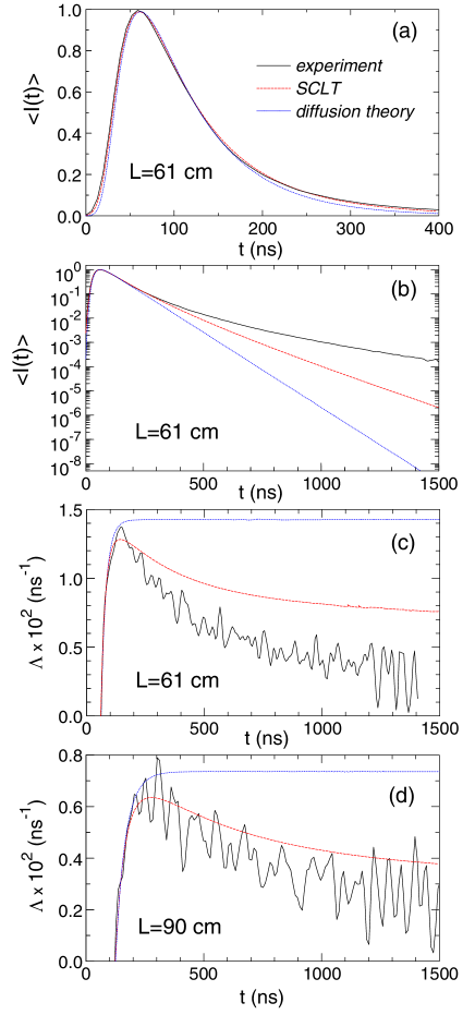
Figure 3: A Gaussian pulse is launched into Q$1$D samples of different sample lengths ($61$ and $90$ cm), and the averaged intensity $\langle I(t)\rangle$ and decay rate $\langle\Lambda(t)\rangle$ on the output plane are measured. The experimental results (solid, in black) are compared with the predictions of the SCLD (namely ‘SCLT’ in panel (a)) model (dashed, in red) and of classical diffusion theory (dotted, in blue). Although the prediction of the SCLD model and the measurements agree well at short times ((a)), dramatic deviations show up at long times ((b)-(d)). The curves are normalized to the peak value in (a) and (b). (from Ref. Zhang09 with reproduction permission from Z. Q. Zhang $\copyright$ The American Physical Society)

In (quasi) one-dimension strong disagreement between the predictions of the SCLD model and measurements in experiments and numerical simulations has been seen Zhang09 ; Tian10 . In the dynamic case, $\tilde{\omega}\neq 0$, both experiments and numerical simulations on the dynamics of microwave pulse propagation through Q$1$D samples have been carried out Zhang09 , and the results of the time-resolved transmission are compared with the prediction of Eqs. (4) and (5). As shown in Fig. 3, although the SCLD model can account very well for the time-resolved transmission at intermediate times, it fails completely at longer times. In the steady state ($\tilde{\omega}=0$), numerical simulations of the wave intensity profile across the sample have been carried out and the local diffusion coefficient was computed Tian10 . The numerical results are compared with the predictions of the SCLD model, and dramatic deviations are found (see Fig. 4).

It has been further shown Zhang09 ; Tian10 that in (quasi) one-dimensional systems transport of localized waves is dominated by rare disorder-induced resonant transmissions which lead to far-reaching consequences (see also Sec. VI). In fact, by using the first-principles microscopic theory it has been shown Tian10 that for $x$ deep inside the samples, i.e., $\xi\ll{\rm min}(x,\,L-x)$,

$$D(x)\sim e^{-\frac{x(L-x)}{L\xi}}.$$ (6)

This result has been fully confirmed by numerical simulations (see Fig. 4). Notice that this expression is symmetric with respect to the sample mid-point, i.e., $D(x)=D(L-x)$. Most importantly, near the sample center, the enhancement from the prediction of the SCLD model is exponentially large $\sim e^{\frac{({\rm min}(x,\,L-x))^{2}}{L\xi}}$. As to be shown in Sec. VI, this dramatic enhancement finds its origin at the novel scaling displayed by $D(x)$ Tian10 . That is, $D(x)$ depends on $x$ via the scaling factor $x(L-x)/(L\xi)$.

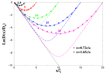
Figure 4: Results of $D(x)/D_{0}$ obtained from numerical simulations (squares and circles), the analytic prediction (6) (solid lines) and the SCLD model (dashed lines) are compared. Numerical simulations are performed for two (angular) wave frequencies, $\omega=1.65c/a$ (square) and $\omega=0.72c/a$ (circle), and for five different sample lengths, $L/\xi=2.5,5,10,15$ and $20$. (from Ref. Tian10 with reproduction permission from C. S. Tian, S. K. Cheung, and Z. Q. Zhang $\copyright$ The American Physical Society)

II.1.3 Is the concept of local diffusion universal?

In some optical systems (e.g., Faraday-active medium Golubentsev84 ; John88 ) the one-loop weak localization may be strongly suppressed and eventually time-reversal symmetry may be broken. In these cases, the SCLD model is no longer applicable since it crucially relies on the one-loop self-consistency or the time-reversal symmetry. On the other hand, there have been rigorous studies showing that systems with/without the time-reversal symmetry (more precisely, corresponding to the Gaussian orthogonal/unitary ensemble (GOE/GUE) in the random matrix theory Beenakker97 ) have largely the same strong localization behavior, and the only difference is the numerical factor of the localization length Efetov83a ; Zirnbauer91 ; Zirnbauer92 ; Zirnbauer94 . An important question therefore arises: Is local diffusion an intrinsic macroscopic phenomenon of (localized) open media? This question was first studied in Ref. Tian10 . By using the first-principles theory to be reviewed below the authors showed that Eq. (6) is valid for both GOE and GUE systems, and the symmetry only affects the numerical coefficient of the localization length, $\xi$.

II.2 Electromagnetic wave propagation: mode picture

Alternatively, transport of waves through open media may be understood in terms of quasi-normal modes. Each quasi-normal mode (labeled by $n$) is characterized by the (complex) wave amplitude, $\varphi_{n}({\bf r})$, the central frequency $\omega_{n}$, and linewidth $\Gamma_{n}>0$. The last represents the rate of wave energy leakage through the interfaces. Upon pumping wave energies into the system, a number of quasi-normal modes are excited, and the wave energies are stored in these modes. In terms of the quasi-normal mode picture, the essential differences between diffusive and localized samples are as follows. For the former system the quasi-normal modes are extended in space, and wave energies are readily transported through the sample. Correspondingly, the lifetimes of quasi-normal modes are short, resulting in a characteristic linewidth greatly exceeding the mean spacing between neighboring eigenfrequencies. For the latter system, there are quasi-normal modes Lifshits79 ; Azbel83 ; Azbel83a whose coupling to outside environments is exponentially small with linewidths much smaller than the mean eigenfrequency spacing. At long times, wave energies are stored mainly in these long-lived modes which therefore play decisive roles in transport of localized waves.

II.2.1 Dynamic single parameter scaling model

Dynamics of localized waves undergoes an essential change in the modal distribution of energy with time: the transmission is mainly due to short-lived overlapping modes at early times and by long-lived localized states at longer times. The long-time dynamics of localized waves is dominated by the spectrally isolated and long-lived localized modes, and is well captured by a phenomenological model, the so-called dynamic single parameter scaling (DSPS) model Zhang09 ; Zhang10 , developed for (quasi) one-dimensional systems.

Consider a one-dimensional sample of length $L\gg\xi$ with transparent interfaces. For a resonantly excited localized mode peaked at a distance $x$ from, say, the left interface ($x=0$), the steady-state intensity at the right interface ($x=L$) relative to the incident wave is Azbel83 ; Azbel83a ,

$$T_{x}=e^{-\gamma(L-2x)},\quad 0<x\leq L/2.$$ (7)

Notice that $T_{x}$ is symmetric with respect to the sample center, i.e., $T_{x}=T_{L-x}$. According to the one-parameter scaling hypothesis Anderson80 , the Lyapunov exponent (namely the inverse localization length) $\gamma$ follows the Gaussian distribution,

$$P(\gamma)=\sqrt{\frac{L\xi}{\pi}}\exp\left[-\frac{L\xi}{4}(\gamma-\xi^{-1})^{2}\right].$$ (8)

For (spectrally isolated and long-lived) localized states, the decay rate is the ratio of the sum of the outgoing fluxes at two interfaces to the integrated wave energy inside the sample,

$$\Gamma(\gamma,x)\sim\gamma\frac{1+e^{-\gamma(L-2x)}}{2e^{\gamma x}-e^{-\gamma(L-2x)}-1}.$$ (9)

Here, an overall numerical factor has been ignored since it is irrelevant for further discussions. Assuming that the modes are uniformly distributed inside the sample, we find the transmitted intensity to be

$$I(t)\equiv I(x=L,t)\sim L^{-1}\int_{4/L}^{\infty}d\gamma\int_{0}^{L/2}dx\,T_{x}\Gamma^{2}e^{-\Gamma t}P(\gamma).$$ (10)

The theoretical prediction of the DSPS model (Eqs. (8) and (9)) for the decay rate $-d\ln I(t)/dt$ is in good agreement with both the experimental measurements and the numerical simulations Zhang09 .

II.2.2 Complete modal analysis

Complete modal analysis has been further performed experimentally by Wang and Genack Genack11 . The underlying general principle is as follows. (In fact, a similar principle has been adopted in studies of transport through quantum chaotic systems, see Ref. Altland10 for a review.) For a linear medium, the wave field, denoted as $E({\bf r},t)$, is the superposition of quasi-normal modes,

$$E({\bf r},t)=\sum_{n}c_{n}\varphi_{n}({\bf r})\,e^{-i(\omega_{n}-i\Gamma_{n})t},$$ (11)

where the coefficients, $c_{n}$’s, are fixed by the initial condition. The wave intensity profile is given by

$$|E({\bf r},t)|^{2}=\sum_{n}|c_{n}\varphi_{n}({\bf r})|^{2}\,e^{-\Gamma_{n}t}+\sum_{n\neq n^{\prime}}c_{n}c_{n^{\prime}}^{*}\varphi_{n}({\bf r})\varphi_{n^{\prime}}({\bf r})^{*}e^{-i(\omega_{n}-\omega_{n^{\prime}})t}e^{-(\Gamma_{n}+\Gamma_{n^{\prime}})t/2}.$$ (12)

The first term is an incoherent contribution reflecting wave transport through individual modes. In contrast, the second term introduces interference between different modes. Since the system is finite, the central frequencies are discrete with a characteristic spacing $\Delta\omega$. At long times, $t\gg 1/\Delta\omega$, the second term becomes negligible and Eq. (12) is simplified to

$$|E({\bf r},t)|^{2}\stackrel{{\scriptstyle t\gtrsim 1/\Delta\omega}}{{\longrightarrow}}\sum_{n}|c_{n}\varphi_{n}({\bf r})|^{2}\,e^{-\Gamma_{n}t}.$$ (13)

This shows that transport at long times is dominated by the long-lived modes with small $\Gamma_{n}$.

It is not an analytic tractable task to obtain complete knowledge on the spectrum and the wave amplitude. Wang and Genack realized Genack11 that quantitative analysis may be substantially simplified in combination with experimental measurements. Experimentally, a pulse is incident from one interface and propagates to the other. The field pattern at the output surface is recorded, which depends only on the coordinates in the transverse plane. According to Eq. (11), it can be decomposed in terms of the so-called volume field speckle pattern, i.e., $c_{n}\varphi_{n}({\bf r})$ with the longitudinal coordinate fixed at $L$. Then, both the spectrum and the corresponding mode speckle pattern can be determined experimentally, see Fig. 1, lower panel for typical intensity spectra which is the squared modular of mode speckle pattern. They in principle afford a full account of dynamic and static transmission. Experiments confirmed a broad range of decay rates and that at long times, the transmission is indeed dominated by incoherent contributions Genack11 .

III ‘Origin’ of supersymmetry

How does the supersymmetry enter into the theory of Anderson localization? In this section we will discuss in a heuristic manner how the supersymmetric trick is prompted in studies of disordered systems particularly in Anderson localization systems Efetov82 ; Efetov82a . Furthermore, we will present some crude technical hints showing how the use of this trick eventually leads us to a supermatrix field theory. The introduction of the supermatrix field lies at the core of nonlinear supermatrix $\sigma$ model theory of localization, as will become clearer in the remainder of this review. To understand the content of this section the readers need to have some basic knowledge on the Grassmann algebra and supermathematics, a preliminary introduction to which is given in Appendix A.

III.1 The supersymmetric trick

Consider a random medium embedded in the air background. Microscopically, the wave field, $E$, is described by the Helmholtz equation John84 ; John85 ; Landau

$$\left\{\nabla^{2}+\omega^{2}(1+\epsilon({\bf r}))\right\}E({\bf r})=0,$$ (14)

where $\omega$ is the (circular) frequency. This equation also describes the propagation of elastic waves John83a ; John83 ; Sheng90 ; Kirkpatrick85 , and is a good approximation Niuwenhuizen to electromagnetic waves provided that the vector character (which is essential, for example, to multiple scattering in a Faraday-active medium in the presence of a magnetic field John89 ; Tiggelen96 ) is unimportant. $\epsilon({\bf r})$ is the fluctuating dielectric field (with zero mean). Interestingly, classical scalar wave equation (14) bears a firm analogy to the Schrödinger equation: ${\hat{H}}\equiv-\nabla^{2}-\omega^{2}\epsilon({\bf r})$ plays the role of the ‘Hamiltonian’ and $\omega^{2}$ the ‘particle energy’. Notice that here the ‘potential’, $\omega^{2}\epsilon({\bf r})$, is ‘energy’-dependent. (The interesting property of the energy-dependence of the potential immediately leads to important consequences of light localization which are profoundly different from electron localization. That is, in the zero frequency limit, the system has an extended state where the wave field is uniform in space. Inheriting from this, in one and two dimension the localization length diverges in the limit $\omega\rightarrow 0$ while in higher dimension the system is extended for sufficiently low $\omega$, see Sec. V.1 for further discussions.)

Let us recall the canonical method of calculating the Green function – the path integral formalism Altland . Specifically, for wave propagation in an infinite random medium described by Eq. (14), similar to quantum mechanics Altland ; Abrikosov65 , we may introduce the retarded (advanced) Green function $G^{R,A}_{\omega^{2}}$ John84 ,

$$(\omega_{\pm}^{2}-{\hat{H}})G^{R,A}_{\omega^{2}}({\bf r},{\bf r}^{\prime})=\delta({\bf r}-{\bf r}^{\prime}),$$ (15)

where $\omega_{\pm}=\omega\pm i\delta$ and $\delta$ is a positive infinitesimal. The fluctuating dielectric $\epsilon({\bf r})$ follows Gaussian distribution with

$$\left\langle\epsilon({\bf r})\epsilon({\bf r}^{\prime})\right\rangle=\Delta({\bf r}-{\bf r}^{\prime}),$$ (16)

where $\Delta({\bf r}-{\bf r}^{\prime})=\Delta(|{\bf r}-{\bf r}^{\prime}|)$ is the correlation function. Then, one may cast the Green functions into the functional integral over some vector field, $\phi_{s}({\bf r}),\,\phi_{s}^{*}({\bf r})$, i.e.,

$$G^{R,A}_{\omega^{2}}({\bf r},{\bf r}^{\prime})=\mp i\frac{\int\phi_{s}({\bf r})\phi_{s}^{*}({\bf r}^{\prime})e^{-S[\phi_{s}]}d[\phi_{s}^{*}]d[\phi_{s}]}{\int e^{-S[\phi_{s}]}d[\phi_{s}^{*}]d[\phi_{s}]}=\mp i\frac{\int d[\phi_{s}^{*}]d[\phi_{s}]\phi_{s}({\bf r})\phi_{s}^{*}({\bf r}^{\prime})e^{-S[\phi_{s}]}}{\int d[\phi_{s}^{*}]d[\phi_{s}]e^{-S[\phi_{s}]}},$$

where $S[\phi_{s}]\equiv\mp i\int d{\bf r}\phi_{s}^{*}(\omega_{\pm}^{2}-{\hat{H}})\phi_{s}$ is a bilinear action. (Throughout this review we use the notation ‘$d[\cdot]$’ or ‘$D[\cdot]$’ to denote the functional measure.) Here, the vector field $\phi_{s}^{*}({\bf r}),\phi_{s}({\bf r})$ are either ordinary complex (with the subscript $s={\rm B}$) or anticommuting (with the subscript $s={\rm F}$) variables. The latter are called Grassmmanians. It should be stressed that for Grassmannians, the complex conjugate is purely formal: an anticommuting variable and its complex conjugate should be understood as independent variables. Notice that throughout this review the independent anticommuting degrees of freedom are even which allows us to freely move the measure under the integral: it can be placed either before or after the integrand.

It is very important that the disorder, i.e., $\omega^{2}\epsilon({\bf r})$, enters into both the denominator (namely the normalization factor) and the numerator of the functional integral. This makes the subsequent disorder average a formidable task. Our aim therefore is to develop a first-principles theory such that disorder is eliminated from the normalization factor. This is accomplished by the supersymmetric trick Efetov82 ; Efetov82a . Specifically, we promote $\phi_{s}({\bf r})$ to a two-component supervector (or graded) field, $\phi({\bf r})$, and $\phi^{*}_{s}({\bf r})$ to $\phi^{\dagger}({\bf r})$, the Hermitian conjugate of $\phi({\bf r})$, i.e., (For simplicity, in this section we ignore the time-reversal symmetry of the Helmholtz equation (14).)

$$\phi({\bf r})\equiv\left(\begin{array}[]{c}\phi_{\rm F}({\bf r})\\ \phi_{\rm B}({\bf r})\\ \end{array}\right),\qquad\phi^{\dagger}({\bf r})\equiv(\phi_{\rm F}^{*}({\bf r}),\phi_{\rm B}^{*}({\bf r})).$$ (19)

As the vector field $\phi_{\rm F}({\bf r})$ ($\phi_{\rm B}({\bf r})$) describes fermionic (bosonic) particles, $\phi({\bf r})$ represents a particle which is a mixture of fermion and boson: the term ‘super’ thereby follows.

By using identity (187) in Appendix A, we may rewrite the Green functions as

$$\pm iG^{R,A}_{\omega^{2}}({\bf r},{\bf r}^{\prime}) = \frac{\delta^{2}{Z}[J^{\dagger},J]}{\delta J_{\rm F}({\bf r}^{\prime})\delta J^{\dagger}_{\rm F}({\bf r})}\bigg{|}_{J^{\dagger},J=0},$$ (20)

$${Z}[J^{\dagger},J] \equiv \int d[\phi^{\dagger}]d[\phi]\exp\left\{-\int d{\bf r}\left(\mp i\phi^{\dagger}({\bf r})(\omega_{\pm}^{2}-{\hat{H}})\phi({\bf r})+J^{\dagger}({\bf r})\phi({\bf r})+\phi^{\dagger}({\bf r})J({\bf r})\right)\right\}.$$

In the absence of the external source, $J^{\dagger}=J=0$, the action is invariant under the unitary transformation in the supervector space: this is the so-called supersymmetry or $\mathbb{Z}_{2}$-grading. The most striking property of Eq. (20) is that $Z[J^{\dagger}=J=0]$ is unity. Indeed, we have here a supermatrix, $M$ (cf. Eq. (171)), as the Gaussian kernel, with the matrix elements $M_{\rm FF}=M_{\rm BB}=\mp i(\omega_{\pm}^{2}-{\hat{H}})$ and $M_{\rm FB}=M_{\rm BF}=0$. From Eq. (186), it follows that in the absence of sources, $J^{\dagger}=J=0$, the partition function $Z={\rm sdet}M={\rm det}(\omega_{\pm}^{2}-{\hat{H}})/{\rm det}(\omega_{\pm}^{2}-{\hat{H}})=1$, where the denominator (numerator) results from the integral over the commuting (anticommuting) variables, $\phi^{*}_{\rm B},\phi_{\rm B}$ ($\phi^{*}_{\rm F},\phi_{\rm F}$). Here, ‘sdet’ stands for the superdeterminant (see Eq. (183) in Appendix A for the definition) and ‘det’ for the ordinary determinant. The striking property of $Z[J^{\dagger}=J=0]=1$ is due to equal number of anticommuting and commuting components. It is this property that (i) leads to a compact expression after disorder averaging (for disorders now enter only into the exponent of the numerator), (ii) keeps the full effect of the disorder averaging, and (iii) renders the theory free of the analytic continuation problem which is encountered in the replica field theory Tian05 ; Efetov97 ; Zirnbauer84 .

In fact, $Z[J^{\dagger}=J=0]=1$ is a special case of the general theorem discovered in Refs. Parisi79 ; Efetov83 ; McKane80 ; Wegner83 . According to this theorem, for a function $f(x)$ satisfying $f(+\infty)<\infty$, we have

$$\int d\phi^{\dagger}d\phi f(\sqrt{(\phi,\phi)})=f(0),$$ (21)

with $\sqrt{(\phi,\phi)}$ being the ‘length’ of the supervector $\phi$ (cf. Eq. (168)). Remarkably, it states that (if the integrand is rotationally invariant in the supervector space,) the integral is given by the value of the integrand at the boundary of integration domain. To apply this theorem to present studies we expand $\phi({\bf r})$ in terms of the eigenmodes of $\hat{H}$, i.e., $\phi({\bf r})=\sum_{n}\phi_{n}\varphi_{n}({\bf r})$, where $\varphi_{n}({\bf r})$ satisfies $\hat{H}\varphi_{n}({\bf r})=\omega^{2}_{n}\varphi_{n}({\bf r})$. Substituting the expansion into $Z$ we find

$${Z}[J^{\dagger}=J=0]=\prod_{n}\int d\phi^{\dagger}_{n}d\phi_{n}e^{\pm i(\omega_{\pm}^{2}-\omega_{n}^{2})\phi^{\dagger}_{n}\phi_{n}}=1,$$ (22)

where the convergence of the integrand is guaranteed by the positive infinitesimal $\delta$.

III.2 Origin of supermatrix field theory

Above we explained the necessity of introducing functional integral over the supervector field if we would wish to get rid of disorders from the normalization factor. But this is not the end of the story. As will become clearer, it is the very beginning instead! Below we will adopt the heuristic approach of Bunder et. al. Zirnbauer05 to explain – in an intuitive manner – why eventually we will deal with an effective theory of supermatrix field, rather than the above-mentioned supervector field. To this end the source term is unimportant and we therefore set $J^{\dagger},J$ to zero.

Let us perform the disorder averaging. As a result,

$$Z\rightarrow\langle Z\rangle=\int d[\phi^{\dagger}]d[\phi]\exp\left\{-\int d{\bf r}d{\bf r}^{\prime}\left[i\phi^{\dagger}({\bf r}^{\prime})\delta({\bf r}^{\prime}-{\bf r})\left(\nabla^{2}+\omega^{2}\right)\phi({\bf r})+\frac{\omega^{4}}{2}\Delta({\bf r}-{\bf r}^{\prime})\left(\phi^{\dagger}({\bf r})\phi({\bf r})\right)\left(\phi^{\dagger}({\bf r}^{\prime})\phi({\bf r}^{\prime})\right)\right]\right\}.$$ (23)

The mathematical structure of the exponent is now undergoing a dramatic change: it is no longer quadratic in the supervector field. Rather, a quartic term appears. The latter may be viewed as the effective interaction among ‘elementary particles’ represented by $\phi$.

On the other hand, experiences have shown that interesting physics in disordered systems arises from multiple scattering. This suggests that we should not treat the ‘interaction’ perturbtively. Instead, we have to keep track of its full effects. To this end, we recall the well-known identity: $\int dx\delta(x-x_{0})=1$. Suppose that its analog,

$$\int D\tilde{Q}({\bf r},{\bf r}^{\prime})\delta(\tilde{Q}({\bf r},{\bf r}^{\prime})-\phi({\bf r})\otimes\phi^{\dagger}({\bf r}^{\prime}))=1$$ (24)

(for all fixed ${\bf r},{\bf r}^{\prime}$), exists in supermathematics. Then, the Dirac function in this ‘identity’ enforces $\tilde{Q}({\bf r},{\bf r}^{\prime})$ to have the same structure as the dyadic product $\phi({\bf r})\otimes\phi^{\dagger}({\bf r}^{\prime})$. Therefore, it must be a supermatrix, i.e.,

$$\tilde{Q}({\bf r},{\bf r}^{\prime})\equiv\left(\begin{array}[]{cc}\tilde{Q}_{\rm FF}({\bf r},{\bf r}^{\prime})&\tilde{Q}_{\rm FB}({\bf r},{\bf r}^{\prime})\\ \tilde{Q}_{\rm BF}({\bf r},{\bf r}^{\prime})&\tilde{Q}_{\rm BB}({\bf r},{\bf r}^{\prime})\\ \end{array}\right).$$ (27)

Here $\tilde{Q}_{\rm FF},\tilde{Q}_{\rm BB}$ ($\tilde{Q}_{\rm FB},\tilde{Q}_{\rm BF}$) are (anti)commuting variables. (More precisely, the former (latter) belongs to the subset ${\cal A}^{+}$ (${\cal A}^{-}$) of the Grassmann algebra and has even (odd) parity, cf. Appendix A.) The measure is defined as $D\tilde{Q}\equiv\pi^{-1}d\tilde{Q}_{\rm FB}d\tilde{Q}_{\rm BF}d\tilde{Q}_{\rm FF}d\tilde{Q}_{\rm BB}$, where we have ignored the arguments ${\bf r},{\bf r}^{\prime}$ to make the formula compact.

Now, let us use the identity (181) to rewrite Eq. (23) as

$$\langle Z\rangle=\int d[\phi^{\dagger}]d[\phi]\exp\left\{\int d{\bf r}d{\bf r}^{\prime}{\rm str}\left[i\delta({\bf r}^{\prime}-{\bf r})\left(\nabla^{2}+\omega^{2}\right)\phi({\bf r})\otimes\phi^{\dagger}({\bf r}^{\prime})+\frac{\omega^{4}}{2}\Delta({\bf r}-{\bf r}^{\prime})(\phi({\bf r})\otimes\phi^{\dagger}({\bf r}^{\prime}))(\phi({\bf r}^{\prime})\otimes\phi^{\dagger}({\bf r}))\right]\right\},$$ (28)

where ‘str’ is the supertrace (see Eq. (179) for the definition). Inserting the ‘identity’ (24) into it, we obtain

$$\langle Z\rangle = \int d[\phi^{\dagger}]d[\phi]\left\{\int D[\tilde{Q}]\delta(\tilde{Q}({\bf r},{\bf r}^{\prime})-\phi({\bf r})\otimes\phi^{\dagger}({\bf r}^{\prime}))\right\}$$ (29)

$$\times\exp\left\{\int d{\bf r}d{\bf r}^{\prime}{\rm str}\left[i\delta({\bf r}^{\prime}-{\bf r})\left(\nabla^{2}+\omega^{2}\right)\phi({\bf r})\otimes\phi^{\dagger}({\bf r}^{\prime})+\frac{\omega^{4}}{2}\Delta({\bf r}-{\bf r}^{\prime})(\phi({\bf r})\otimes\phi^{\dagger}({\bf r}^{\prime}))(\phi({\bf r}^{\prime})\otimes\phi^{\dagger}({\bf r}))\right]\right\}.$$

Suppose that it is legitimate to exchange the integral order. Integrating out the $\phi$-field first gives

$$\langle Z\rangle=\int D[\tilde{Q}]J[\tilde{Q}]\exp\left\{\int d{\bf r}d{\bf r}^{\prime}{\rm str}\left[i\delta({\bf r}^{\prime}-{\bf r})\left(\nabla^{2}+\omega^{2}\right)\tilde{Q}({\bf r},{\bf r}^{\prime})+\frac{\omega^{4}}{2}\Delta({\bf r}-{\bf r}^{\prime})\tilde{Q}({\bf r},{\bf r}^{\prime})\tilde{Q}({\bf r}^{\prime},{\bf r})\right]\right\},$$ (30)

where we have used the ‘identity’: $\int D\tilde{Q}\delta(\tilde{Q}-\phi\otimes\phi^{\dagger})f(\phi\otimes\phi^{\dagger})\equiv\int D\tilde{Q}\delta(\tilde{Q}-\phi\otimes\phi^{\dagger})f(\tilde{Q})$ and

$$J[\tilde{Q}({\bf r},{\bf r}^{\prime})]\equiv\int d\phi^{\dagger}({\bf r}^{\prime})d\phi({\bf r})\delta(\tilde{Q}({\bf r},{\bf r}^{\prime})-\phi({\bf r})\otimes\phi^{\dagger}({\bf r}^{\prime})).$$ (31)

The latter is the analog of the well-known identity: $\int dx\delta(f(x))=\sum_{i}|f^{\prime}(x_{i})|^{-1}$ with $f(x_{i})=0$.

Thus, we have achieved an important result: disorder-averaged correlation functions can be traded to a functional integral over a supermatrix field. This is the core of the so-called superbosonization Zirnbauer05 . Nevertheless, the above derivations are intuitive and largely formal. In particular, we have paid no attention to the mathematical foundation of manipulations with the Dirac function of supermatrices. In fact, the superbosonization can be established on the level of mathematical rigor without involving the Dirac function of Grassmannians Zirnbauer05 . However, this requires advanced knowledge on supermathematics and we shall not proceed further here. In the next section, we will follow the more conventional route of using the super-Hubbard–Stratonovich (HS) transformation to introduce the supermatrix field, which was first done by Efetov Efetov83 .

IV Supersymmetric field theory of light localization in open media

In the remainder of this review, we will study wave propagation in large scales by using the supersymmetric field theoretic approach. Due to the interplay between wave interference and wave energy leakage through the air-medium interface, localization physics of classical waves in an open medium is even richer in comparison to that in an infinite medium. At the technical level, the corresponding field-theoretic description dramatically differs from that for infinite media. In this section, we will review the supersymmetric field theory of light localization in random open media developed in Ref. Tian08 . We will first reproduce the supermatrix $\sigma$ model of Efetov in the context of classical waves in an infinite medium; Then, we will derive the air-medium coupling action that crucially constrains the supermatrix field on the interface.

In reality, localization properties are probed by quantities such as the correlation function ${\cal Y}({\bf r},{\bf r}^{\prime};\tilde{\omega})$, the wave intensity distribution Mirlin00 , the transmission distribution Dorokhov82 ; Mello88 ; Frahm95 ; Rejaei96 ; Zirnbauer04 ; Tian05 , etc.. The microscopic expressions of these observables involve the product of the retarded and advanced Green functions. Thus, we have to double the supervector so as to account for the distinct analytic structures of these two Green functions: this defines the advanced/retarded (‘ar’) space, with index $m=1,2$. Because Helmholtz equation (14) is invariant with respect to the time-reversal operation (the complex conjugation), we may consider the wave field and its complex conjugate as independent variables. To accommodate this degree of freedom we need to further double the supervector, which defines the time-reversal (‘tr’) space, with index $t=1,2$. Finally, the doubling (19) defines the fermionic/bosonic (‘fb’) space, with index $\alpha={\rm F},\,{\rm B}$. We have thereby introduced an $8$-component supervector field $\psi({\bf r})=\{\psi_{m\alpha t}({\bf r})\}$.

IV.1 Nonlinear supermatrix $\sigma$ model for infinite media

Let us start from the case of infinite media. It is necessary to reproduce the nonlinear supermatrix $\sigma$ model for light localization and discuss substantially the underlying technical ideas. The reasons are as follows. (i) Although the derivations for classical scalar waves are largely parallel to those of (spinless) de Broglie waves Efetov97 , below many detailed treatments are different from Ref. Efetov97 . (ii) In doing so, we wish to show that the mathematical rigor of the nonlinear $\sigma$ model must be understood correctly. That is, it is not a ‘rigorous’ mapping of the microscopic equation (14); rather, it is an effective (low-energy) theory derived from the latter under some parametric conditions. (iii) Although the low-energy field theory turns out to be the same for classical and de Broglie waves, the conditions justifying such a theory are not. This leads to far-reaching consequences. In fact, as we will see below, localization physics of light differs from that of de Broglie waves in many important aspects. Therefore, it is necessary to have at our disposal a complete list of these conditions. (iv) Reflections of the derivations may provide significant insights into developing a first-principles localization theory incorporating vector wave character and (or) linear gain effects. Both are fundamental issues in studies of classical electromagnetic wave localization. (v) Although theoretical works using the supersymmetric field theory to study light localization have appeared, as mentioned in the introductory part, to the best of my knowledge, detailed derivations of this theory in the context of classical waves have so far been absent. (vi) We hope that a technical review on the nonlinear supermatrix $\sigma$ model of light localization in infinite media may help the readers unfamiliar with Efetov’s theory to better appreciate how this technique unifies mathematical rigor and physical transparency, and powerful it is in studying light localization.

Similar to Eq. (20), one may express the product of the retarded and advanced Green function in terms of certain derivative of the partition function, ${\cal Z}[J^{\dagger},J]$, with respect to the source, $J^{\dagger}({\bf r}),J({\bf r})$. The partition function is now a functional integral over the supervector field, $\psi$, and its Hermitian conjugate, $\psi^{\dagger}$,

$${\cal Z}[J^{\dagger},J]\equiv z\int d[\psi^{\dagger}]d[\psi]\left\langle\exp\left\{-\int d{\bf r}\left[i\psi^{\dagger}K\left(\nabla^{2}+\omega^{2}+\omega^{2}\epsilon({\bf r})-\omega\tilde{\omega}^{+}\Lambda\right)\psi+J^{\dagger}K\psi+\psi^{\dagger}KJ\right]\right\}\right\rangle,$$ (32)

where $\Lambda\equiv\sigma_{3}^{\rm ar}\otimes{\mathbbm{1}}^{\rm fb}\otimes{\mathbbm{1}}^{\rm tr}$, with $\sigma_{i}^{X},\,i=0,1,2,3$ and $\sigma_{0}^{X}\equiv{\mathbbm{1}}^{X}$ the Pauli matrices defined on the space $X=$‘ar’, ‘fb’, and ‘tr’, $K$ is a metric tensor, and to make the formula compact we have dropped out the arguments of the fields. The numerical coefficient $z$ depends on the metric tensor $K$. Similar to the example discussed in Sec. III.1, this normalization factor is independent of disorder Zirnbauer85 , and its explicit value is not given here since it does not affect the subsequent analysis. We will postpone giving the explicit form of the metric tensor till Sec. IV.1.3. At this moment we merely mention that the choice of $K$ ensures the convergence of the above functional integral. In deriving Eq. (32) we have omitted all the $\tilde{\omega}^{2}$ terms, since we are interested in large-scale physics where the characteristic time ($\sim\tilde{\omega}^{-1}$) is much larger than the inverse (angular) frequency $\omega^{-1}$, i.e.,

$$\tilde{\omega}\ll\omega.$$ (33)

To proceed further, we consider a simpler case for dielectric fluctuations, i.e., $\Delta({\bf r}-{\bf r}^{\prime})=\Delta\,\delta({\bf r}-{\bf r}^{\prime})$ with $\Delta$ being the disorder strength. Performing the disorder averaging, we obtain

$${\cal Z}[J^{\dagger},J]=z\int d[\psi^{\dagger}]d[\psi]\exp\left\{-\int d{\bf r}\left[i\psi^{\dagger}K\left(\nabla^{2}+\omega^{2}-\omega\tilde{\omega}^{+}\Lambda\right)\psi+\frac{\Delta\omega^{4}}{2}\left(\psi^{\dagger}K\psi\right)^{2}+J^{\dagger}K\psi+\psi^{\dagger}KJ\right]\right\}.$$ (34)

Importantly, in the absence of the frequency and source terms, i.e., $\tilde{\omega}^{+}=J^{\dagger}=J=0$, the action namely the exponent is invariant under the gauge transformation $U$: $\psi\rightarrow U\psi$, provided that $U$ preserves the metric tensor, i.e.,

$$U^{\dagger}KU=K.$$ (35)

Furthermore, by the construction of the supervector field it satisfies the ‘reality condition’,

$$\psi^{\dagger}=(C\psi)^{\rm T},\quad C=\left(\begin{array}[]{cc}-i\sigma_{2}^{\rm tr}&0\\ 0&\sigma_{1}^{\rm tr}\\ \end{array}\right)^{\rm fb}\otimes{\mathbbm{1}}^{\rm ar},$$ (38)

where the superscript, ‘T’, stands for the transpose. Its invariance under the gauge transformation requires

$$U^{\dagger}=CU^{\rm T}C^{\rm T}.$$ (39)

All the supermatrices $U$ satisfying Eqs. (35) and (39) constitute the symmetry group of the system and is denoted as $G$.

IV.1.1 Effective interactions and low-momentum transfer channels

Similar to Eq. (23), the action in Eq. (34) describes the dynamics of an ‘elementary particle’ which is a mixture of fermion and boson. Remarkably, the quartic term – arising from the disorder averaging – introduces the effective interaction between elementary particles. Written in terms of the components of the supervector, it is

$$\frac{\Delta\omega^{4}}{2}\,\int d{\bf r}\left(\psi^{\dagger}K\psi\right)^{2} = \frac{\Delta\omega^{4}}{2}\,\int d{\bf r}\psi^{\dagger}_{i}K_{ij}\left(\psi^{\dagger}_{i^{\prime}}K_{i^{\prime}j^{\prime}}\psi_{j^{\prime}}\right)\psi_{j}$$ (40)

$$= \frac{\Delta\omega^{4}}{2}\,\int d{\bf r}\psi^{\dagger}_{i}K_{ij}\left(\psi_{j}\otimes\psi^{\dagger}_{i^{\prime}}K_{i^{\prime}j^{\prime}}\right)\psi_{j^{\prime}}$$

$$= \frac{\Delta\omega^{4}}{2}\,\int d{\bf r}\psi_{i}(-kK)^{\rm T}_{ij}\left(\psi^{\dagger}_{j}\otimes\psi^{\dagger}_{i^{\prime}}K_{i^{\prime}j^{\prime}}\right)\psi_{j^{\prime}},$$

with $k=\sigma_{3}^{\rm fb}$ which accounts for the anticommutating relation of Grassmannians. Here, the subscripts $i,j,\cdots$ are the abbreviations of the index $(m\alpha t)$ of the supervector components, and the Einstein summation convention applies to the index. Recall that if the elementary particle is coupled to an external field, $(V_{\rm ext})_{ij}$, then the action acquires an additional term $\int d{\bf r}\psi^{\dagger}_{i}K_{ij}(V_{\rm ext})_{jk}\psi_{k}$ (see, for example, the $\omega\tilde{\omega}^{+}\Lambda$ term in the action). Comparing this structure with the interaction (40), we see that the particle self-generates some effective fields dictating the particle’s motion. Specifically, the first equality suggests an effective scalar field $\sim\psi^{\dagger}_{i}K_{ij}\psi_{j}$ (because this is a number), while the other two (which are related to each other via the reality condition (38)) of a supermatrix structure $\sim\psi\otimes\psi^{\dagger}K$ (because this is a dyadic product).

In the Fourier representation, these self-generated fields are decomposed into slow and fast modes: the former fluctuates over a scale much larger than the mean free path $l$, with $q=|{\bf q}|$ (${\bf q}$ being the Fourier wave number) much smaller than $l^{-1}$; while the latter over a scale $\lesssim l$ with $q\gtrsim l^{-1}$. (For ballistic samples, where the mean free path and the system size are comparable, the fast-slow mode decomposition becomes very subtle, and it turns out that a low-energy theory is totally different from that to be derived below. We shall not discuss this issue further, and refer readers to the original papers Khmelnitskii94 ; Andreev96 ; Andreev97 and the monograph Khmelnitskii97 .) The slow mode possesses mathematical structure inheriting from the self-generated fields. Each slow-mode structure defines a specific low-momentum (i.e., $ql\ll 1$) transfer channel. To illustrate this we pass to the Fourier representation and rewrite Eq. (40) as

$$\frac{\Delta\omega^{4}}{2}\,\int d{\bf r}\left(\psi^{\dagger}K\psi\right)^{2} = \frac{\Delta\omega^{4}}{2}\,\int\frac{d{\bf k}}{(2\pi)^{d}}\frac{d{\bf k}^{\prime}}{(2\pi)^{d}}\frac{d{\bf q}}{(2\pi)^{d}}\,\psi^{\dagger}_{{\bf k}}K\left(\psi^{\dagger}_{{\bf k}^{\prime}}K\psi_{-{\bf k}^{\prime}-{\bf q}}\right)\psi_{-{\bf k}+{\bf q}}$$ (41)

$$= \frac{\Delta\omega^{4}}{2}\,\int\frac{d{\bf k}}{(2\pi)^{d}}\frac{d{\bf k}^{\prime}}{(2\pi)^{d}}\frac{d{\bf q}}{(2\pi)^{d}}\,\psi^{\dagger}_{{\bf k}}K\left(\psi_{{\bf k}^{\prime}}\otimes\psi^{\dagger}_{-{\bf k}^{\prime}-{\bf q}}K\right)\psi_{-{\bf k}+{\bf q}}$$

$$= \frac{\Delta\omega^{4}}{2}\,\int\frac{d{\bf k}}{(2\pi)^{d}}\frac{d{\bf k}^{\prime}}{(2\pi)^{d}}\frac{d{\bf q}}{(2\pi)^{d}}\,\psi^{\rm T}_{{\bf k}}K^{\rm T}\left(-k(\psi^{\dagger}_{{\bf k}^{\prime}})^{\rm T}\otimes\psi^{\dagger}_{-{\bf k}^{\prime}-{\bf q}}K\right)\psi_{-{\bf k}+{\bf q}}.$$

Here, $\psi_{\bf k}$ ($\psi^{\dagger}_{\bf k}$) is the Fourier transformation of $\psi$ ($\psi^{\dagger}$), and stands for annihilating (creating) an elementary particle of momentum ${\bf k}$ (-${\bf k}$). Notice that the interaction conserves the total momentum. Each equality above is respectively represented by an interaction vertex shown in Fig. 5 (a)-(c). The entity of two green (blue) lines defines a channel through which a momentum ${\bf q}$ is transferred. (With the momentum ${\bf k}$ or ${\bf k}^{\prime}$ integrated out,) it varies over a scale $\sim 1/q\gg l$. Therefore, the entity specifies a slow-mode structure, and the interaction introduces the slow-mode coupling.

Importantly, since the transferred momentum is small enough, i.e., $ql\ll 1$, these three channels do not overlap. Following Ref. Altland we call the first, (a), the direct channel. Two particles undergoing scattering due to this interaction acquire a small momentum change ${\bf q}$ (or $-{\bf q}$). The second, (b), may be called the diffuson (or exchange following the term of Ref. Altland ) channel and the third, (c), the cooperon channel. In fact, if the momentum ${\bf q}$ transfer through the second (third) channel occurs successively, then a diagram represented by (d) ((e)) results, which is the prototype of the well-known diffuson (cooperon) in the diagrammatic perturbation theory Woelfle92 ; Altland . Technically, the latter may be achieved by inserting Eq. (41) with corresponding low-momentum transfer channel into Eq. (34), expanding the quartic term and summing up the infinite series.

The fast modes do not affect large-scale physics, and the interaction is dominated by the slow modes,

$$\frac{\Delta\omega^{4}}{2}\,\int\left(\psi^{\dagger}K\psi\right)^{2}d{\bf r}\approx\frac{\Delta\omega^{4}}{2}\int^{\prime}\frac{d{\bf k}}{(2\pi)^{d}}\frac{d{\bf k}^{\prime}}{(2\pi)^{d}}\frac{d{\bf q}}{(2\pi)^{d}}\,\psi^{\dagger}_{{\bf k}}K\left(\psi^{\dagger}_{{\bf k}^{\prime}}K\psi_{-{\bf k}^{\prime}-{\bf q}}+2\psi_{{\bf k}^{\prime}}\otimes\psi^{\dagger}_{-{\bf k}^{\prime}-{\bf q}}K\right)\psi_{-{\bf k}+{\bf q}},$$ (42)

with $\int^{\prime}\equiv\int_{ql\ll 1}$, where the factor two results from the reality condition (38) namely the reciprocal relation between the diffuson and cooperon channel. Define

$$J_{{\bf q}}\equiv\int\frac{d{\bf k}}{(2\pi)^{d}}\psi^{\dagger}_{{\bf k}}K\psi_{-{\bf k}+{\bf q}},\qquad M_{{\bf q}}\equiv\int\frac{d{\bf k}}{(2\pi)^{d}}\psi_{{\bf k}}\otimes\psi^{\dagger}_{-{\bf k}+{\bf q}}K,$$ (43)

we write Eq. (42) as

$$\frac{\Delta\omega^{4}}{2}\,\int\left(\psi^{\dagger}K\psi\right)^{2}d{\bf r}\approx\frac{\Delta\omega^{4}}{2}\int^{\prime}\frac{d{\bf q}}{(2\pi)^{d}}\,J_{{\bf q}}J_{-{\bf q}}-\Delta\omega^{4}\int^{\prime}\frac{d{\bf q}}{(2\pi)^{d}}\,{\rm str}(M_{{\bf q}}M_{-{\bf q}}),$$ (44)

where in obtaining the second term we have used the identity (181).

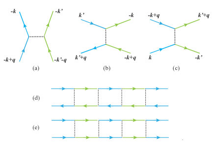
Figure 5: The (effective) particle-particle interaction may result in a small momentum (${\bf q}$) transfer via the direct (a), the diffuson or exchange (b), or the cooperon (c) channel. Successive small momentum transfer via the second (third) channel leads to a ladder diagram (d) ((e)), which is the prototype of the diffuson (cooperon) in the diagrammatic perturbation theory. The dashed line representing the interaction enforces two spatial coordinates involved to be identical, reflecting the $\delta$-correlation nature of disorders.

IV.1.2 Introduction of the supermatrix $Q$-field

The two exponents, $I_{1}\equiv\exp\left(-\frac{\Delta\omega^{4}}{2}\int^{\prime}\frac{d{\bf q}}{(2\pi)^{d}}\,J_{{\bf q}}J_{-{\bf q}}\right)$ and $I_{2}\equiv\exp\left\{\Delta\omega^{4}\int^{\prime}\frac{d{\bf q}}{(2\pi)^{d}}\,{\rm str}(M_{{\bf q}}M_{-{\bf q}})\right\}$, can be decoupled via the HS decoupling which transforms a quartic interaction into a quadratic one. The super-HS decoupling below for the quartic interaction of the supervector field was introduced by Efetov (see Refs. Efetov83 ; Efetov97 for a technical review and the original derivations). Here, we wish to adopt the treatments of Ref. Zirnbauer84 .

By inserting the identity:

$$1\equiv{\cal N}/{\cal N},\quad{\cal N}\equiv\int D[{\cal E}_{{\bf q}}]\exp\left\{-\frac{1}{2\Delta}\int^{\prime}\frac{d{\bf q}}{(2\pi)^{d}}{\cal E}_{{\bf q}}{\cal E}_{-{\bf q}}\right\}$$ (45)

into $I_{1}$, we obtain

$$I_{1}={\cal N}^{-1}\int D[{\cal E}_{{\bf q}}]\exp\left\{-\frac{1}{2\Delta}\int^{\prime}\frac{d{\bf q}}{(2\pi)^{d}}{\cal E}_{{\bf q}}{\cal E}_{-{\bf q}}\right\}\exp\left(-\frac{\Delta\omega^{4}}{2}\int^{\prime}\frac{d{\bf q}}{(2\pi)^{d}}\,J_{{\bf q}}J_{-{\bf q}}\right),$$ (46)

where ${\cal E}_{-{\bf q}}={\cal E}_{\bf q}^{*}$. Then, for the integral we make the change of variable: ${\cal E}_{{\bf q}}\rightarrow{\cal E}_{{\bf q}}+i\Delta\omega^{2}J_{{\bf q}}$ which does not affect the convergence. As a result,

$$I_{1}={\cal N}^{-1}\int D[{\cal E}_{{\bf q}}]\exp\left\{-i\omega^{2}\int^{\prime}\frac{d{\bf q}}{(2\pi)^{d}}{\cal E}_{-{\bf q}}J_{{\bf q}}-\frac{1}{2\Delta}\int^{\prime}\frac{d{\bf q}}{(2\pi)^{d}}{\cal E}_{{\bf q}}{\cal E}_{-{\bf q}}\right\}.$$ (47)

Therefore, we achieve the HS decoupling in the direct channel: on the right-hand side the action is linear in $J_{\bf q}$. Conjugate to the ‘external’ field structure $\sim\psi^{\dagger}K\psi$ which is a commuting variable (because Grassmannians appear in pairs), the decoupling field ${\cal E}_{\bf q}$ is a complex scalar field. This is the ordinary HS decoupling Altland .

For the exponent $I_{2}$, by inserting the unity:

$$1\equiv\int D[Q_{\bf q}]\exp\left\{-\Delta^{-1}\int^{\prime}\frac{d{\bf q}}{(2\pi)^{d}}\,{\rm str}(Q_{{\bf q}}Q_{-{\bf q}})\right\},$$ (48)

where the supermatrix $Q_{\bf q}$ has the same symmetry structure as the dyadic product $\psi\otimes\psi^{\dagger}K$, and the convergence is assumed, we obtain

$$I_{2}=\int D[Q_{\bf q}]\exp\left\{-\Delta^{-1}\int^{\prime}\frac{d{\bf q}}{(2\pi)^{d}}\,{\rm str}(Q_{{\bf q}}Q_{-{\bf q}})+\Delta\omega^{4}\int^{\prime}\frac{d{\bf q}}{(2\pi)^{d}}\,{\rm str}(M_{{\bf q}}M_{-{\bf q}})\right\}.$$ (49)

Making the variable transformation: $Q_{{\bf q}}\rightarrow Q_{{\bf q}}-\Delta\omega^{2}M_{{\bf q}}$, we find

$$I_{2}=\int D[Q_{\bf q}]\exp\left\{2\omega^{2}\int^{\prime}\frac{d{\bf q}}{(2\pi)^{d}}\,{\rm str}(M_{{\bf q}}Q_{-{\bf q}})-\Delta^{-1}\int^{\prime}\frac{d{\bf q}}{(2\pi)^{d}}\,{\rm str}(Q_{{\bf q}}Q_{-{\bf q}})\right\}.$$ (50)

This is the super-HS decoupling in the diffuson-cooperon channel: on the right-hand side the action is linear in $M_{\bf q}$. In contrast to Eq. (47), the super-HS decoupling in the diffuson-cooperon channel has a normalization factor of unity. This is a consequence of equal commuting (anticommuting) degrees of freedom which can be easily found to be $16$ by explicitly writing down the matrix elements of the dyadic product $\psi\otimes\psi^{\dagger}$.

Combining the HS decouplings (47) and (50), we have

$$e^{-\frac{\Delta\omega^{4}}{2}\,\int\left(\psi^{\dagger}K\psi\right)^{2}d{\bf r}}$$ (51)

$$= {\cal N}^{-1}\int D[{\cal E}_{{\bf q}}]\exp\left\{-i\omega^{2}\int^{\prime}\frac{d{\bf q}}{(2\pi)^{d}}\int\frac{d{\bf k}}{(2\pi)^{d}}{\cal E}_{-{\bf q}}\psi^{\dagger}_{{\bf k}}K\psi_{-{\bf k}+{\bf q}}-\frac{1}{2\Delta}\int^{\prime}\frac{d{\bf q}}{(2\pi)^{d}}{\cal E}_{{\bf q}}{\cal E}_{-{\bf q}}\right\}$$

$$\times \int D[Q_{{\bf q}}]\exp\left\{-2\omega^{2}\int^{\prime}\frac{d{\bf q}}{(2\pi)^{d}}\int\frac{d{\bf k}}{(2\pi)^{d}}\psi^{\dagger}_{{\bf k}}KQ_{-{\bf q}}\psi_{-{\bf k}+{\bf q}}-\Delta^{-1}\int^{\prime}\frac{d{\bf q}}{(2\pi)^{d}}{\rm str}Q_{{\bf q}}Q_{-{\bf q}}\right\}.$$

In the derivation above we have used the identity (181). Most importantly, by the HS decoupling we transfer the interaction – a quartic term – into an action quadratic in $\psi$. The price is the introduction of two new fields, the complex scalar field ${\cal E}_{{\bf q}}$ and the supermatrix field $Q_{{\bf q}}$.

Let us substitute Eq. (51) into Eq. (34). For the first line of Eq. (51), the first term in the exponent of the numerator is to locally renormalize the average refractive index, i.e., $\omega^{2}\rightarrow\omega^{2}(1+{\cal E}({\bf r}))$, which is negligible. Therefore, the normalization factor ${\cal N}$ and the functional integral over ${\cal E}_{{\bf q}}$ cancel. That is, the decoupling in the direct channel gives a trivial factor of unity and plays no roles. As a result, upon passing to the real space representation, we obtain

$$\exp\left\{-\frac{\Delta\omega^{4}}{2}\,\int\left(\psi^{\dagger}K\psi\right)^{2}\,d{\bf r}\right\}=\int D[Q]\exp\left\{-\int\left(2\omega^{2}\psi^{\dagger}KQ\psi+\Delta^{-1}{\rm str}Q^{2}\right)d{\bf r}\right\}.$$ (52)

Notice that the $Q$-field is composed of slow modes and therefore varies over a scale much larger than the mean free path. Thanks to Eq. (35) the exponent of the right-hand side is invariant under the global (in the sense that the transformation is uniform in space) gauge transformation: $\psi\rightarrow U\psi,\,Q\rightarrow U^{-1}QU,\,U\in G$.

Then, we insert Eq. (52) into Eq. (34). For the action is quadratic in $\psi$, we may integrate out this field exactly, obtaining (That to exchange the order of integration is legitimate is guaranteed by appropriate choice of the metric tensor $K$, see Sec. IV.1.3 for further discussions.)

$${\cal Z}=\int D[Q]e^{-F[Q]-F_{J}[Q]}.$$ (53)

Here, the action

$$F[Q]=\int d{\bf r}\,{\rm str}\left\{\Delta^{-1}Q^{2}-\frac{1}{2}\ln\left[-\nabla^{2}-\omega^{2}+\omega\tilde{\omega}^{+}\Lambda+2i\omega^{2}Q\right]\right\}.$$ (54)

$F_{J}[Q]$ is the source-dependent action whose details rely on specific physical observable used to characterize the system’s localization behavior and do not affect localization physics. Since we are interested in the general structure of the low-energy field theory in this section, we do not pay attention to its explicit form. Importantly, although the functional measure formally includes both $\psi^{\dagger}$ and $\psi$, the reality condition (38) reduces the independent degrees of freedom by one half, which leads to the pre-logarithmic factor $\frac{1}{2}$ in Eq. (54). Equations (53) and (54) cast physical observables into an expression in terms of the functional integral over the supermatrix field, $Q({\bf r})$. In the absence of the $\omega\tilde{\omega}^{+}\Lambda$ term and the external source namely $F_{J}[Q]$, the action in Eq. (53) is invariant under the global gauge transformation: $Q\rightarrow U^{-1}QU$ where $U\in G$ is homogeneous in space.

IV.1.3 Nonlinear supermatrix $\sigma$ model

We then consider the functional integral over the $Q$-field. Again we ignore the source term, $F_{J}[Q]$, for the same reasons as above. The program is first to find the saddle points (denoted as $Q_{0}$) of the action $F[Q]|_{\tilde{\omega}^{+}=0}$ and then to integrate out (Gaussian) fluctuations around them. Let us substitute $Q=Q_{0}+\delta Q$ into the action $F[Q]|_{\tilde{\omega}^{+}=0}$ and expand it in terms of the deviation, $\delta Q$. Demanding the linear term to vanish gives

$$Q_{0}({\bf r})=\frac{1}{2}\omega^{2}\Delta\mathcal{G}_{0}({\bf r},{\bf r};Q_{0}),\quad\mathcal{G}_{0}({\bf r},{\bf r}^{\prime};Q)\equiv i\langle{\bf r}|(-\nabla^{2}-\omega^{2}+2i\omega^{2}Q)^{-1}|{\bf r}^{\prime}\rangle.$$ (55)

The imaginary part of the matrix Green function $\mathcal{G}_{0}$ implies that it decays exponentially when the distance $|{\bf r}-{\bf r}^{\prime}|$ is greater than a characteristic length which, as we will see below, is the elastic mean free path. In Appendix B, we show that for low frequencies, i.e.,

$$\Delta\omega\nu(\omega)\ll 1\Leftrightarrow\omega\ll\Delta^{-1/d}$$ (56)

with $\nu(\omega)\sim\omega^{d-1}$ being the density of states of free photons, diagonalizing Eq. (55) leads to two saddle points, $\tilde{q}\Lambda$ and $\tilde{q}(-k\Lambda)$, uniform in space (the ‘mean field’ saddle points), where $\tilde{q}\equiv\frac{\pi}{4}\Delta\omega\nu(\omega)$. It is important to notice that these are not the complete solutions to Eq. (55). Indeed, this equation is invariant under the rotation, $Q_{0}\rightarrow T^{-1}Q_{0}T,\,T\in G$, and the two saddle points, $\tilde{q}\Lambda$ and $\tilde{q}(-k\Lambda)$, are connected via this rotation. Therefore, the solutions to Eq. (55) constitute a manifold,

$$Q=\tilde{q}\,T^{-1}\Lambda T.$$ (57)

As shown in Ref. Zirnbauer84 , enforced by the convergence of the functional integral over $\psi,\psi^{\dagger},Q$ and the analytic structure of the saddle point, the boson-boson (fermion-fermion) block in the fb-space is invariant under the non-compact (compact) group of transformations. This fixes the metric tensor (in its diagonal form),

$$K=\left(\begin{array}[]{cc}{\mathbbm{1}}^{\rm fb}&0\\ 0&\sigma_{3}^{\rm fb}\\ \end{array}\right)^{{\rm ar}}\otimes{\mathbbm{1}}^{\rm tr}.$$ (60)

Combined with Eqs. (35) and (39), this defines the symmetry group $G=UOSP(2,2|4)$ for the orthogonal ensemble Zirnbauer85 , which is a pseudounitary supergroup. The notation to the left (right) of ‘$|$’ stands for the metric in the bosonic (fermionic) sector: ‘$2,2$’ refers to the hyperbolic metric, $(+,+,-,-)$ and ‘$4$’ to the Euclidean metric, $(+,+,+,+)$. Importantly, there is a subgroup $H\subset G$ which is a direct product of two unitary groups, $UOSP(2|2)$, defined in the advanced-advanced and retarded-retarded block, respectively. Elements of $H$ generate rotation rendering $\Lambda$ invariant. In this sense, elements of $H$ may be considered to be identical. More precisely, in Eq. (57) $T$ takes the value from the coset space, i.e.,

$$T\in G/H=UOSP(2,2|4)/UOSP(2|2)\otimes UOSP(2|2).$$ (61)

As we will discuss in details in Sec. IV.3, breaking of this global continuous symmetry leads to gapless collective modes, the so-called Goldstone modes. It is these modes, known as diffusons and cooperons in the perturbative diagrammatic technique Woelfle80a ; Woelfle80 ; Larkin79 , and their interactions that carry the full information on localization physics. This will be established in the following sections. We now proceed to analyze the action of these modes.

Since we are interested in low-energy physics, the coupling between the $Q$-field spatial fluctuations and finite frequency ($\tilde{\omega}^{+}\neq 0$) effects is negligible, (The latter characterizes dynamic effects of fluctuations.) and they contribute separately to the effective action. To find the contribution of the former we set $\tilde{\omega}^{+}=0$. Recall that the first order term in the $\delta Q$-expansion vanishes. By keeping the expansion up to the second order we find the fluctuation action,

$$\int\frac{d{\bf q}}{(2\pi)^{d}}{\rm str}\left\{\omega^{4}\int\frac{d{\bf k}}{(2\pi)^{d}}{\cal G}_{0}\left({\bf k}+\frac{{\bf q}}{2},Q_{0}\right)\delta Q_{\bf q}{\cal G}_{0}\left({\bf k}-\frac{{\bf q}}{2},Q_{0}\right)\delta Q_{-{\bf q}}+\Delta^{-1}\delta Q_{\bf q}\delta Q_{-{\bf q}}\right\},$$ (62)

where we have passed to the Fourier representation: $\delta Q({\bf r})\rightarrow\delta Q_{{\bf q}}$ and ${\cal G}_{0}\left({\bf r},{\bf r}^{\prime},Q_{0}\right)\rightarrow{\cal G}_{0}\left({\bf k},Q_{0}\right)$. (Notice that according to Eq. (55), ${\cal G}_{0}\left({\bf r},{\bf r}^{\prime},Q_{0}\right)$ is translationally invariant, i.e., ${\cal G}_{0}\left({\bf r},{\bf r}^{\prime},Q_{0}\right)={\cal G}_{0}\left({\bf r}-{\bf r}^{\prime},Q_{0}\right)$.) Suppose first that $Q_{0}=\Lambda$. We see that fluctuations around it can be decomposed into two components: one commutes with it while the other anticommutes. Since the (anti)commutation relation is invariant under the global rotation, we may rotate $\Lambda$ to arbitrary $Q_{0}$ in the saddle point manifolds. At the same time, we obtain two fluctuation components, the longitudinal ($\delta Q_{\bf q}^{l}$) and transverse ($\delta Q_{\bf q}^{t}$) components: the former (latter) commutes (anticommutes) with $Q_{0}$. Physically, fluctuations along the transverse directions move $Q_{0}$ to somewhere the saddle point manifold (cf. Eqs. (57) and (61)), while fluctuations along the longitudinal directions bring $Q_{0}$ out of the saddle point manifold (see Appendix C for further explanations).

Let us substitute the decomposition into Eq. (62). Integrating out the longitudinal components, $\delta Q_{{\bf q}}^{l}$, gives a factor of unity. We are left with a functional integral over the transverse component, $\delta Q_{{\bf q}}^{t}$. Upon passing to real space, this gives the fluctuation action (see Appendix C for details),

$$\delta F_{1}\equiv\frac{\pi\nu D_{0}}{8}\int d{\bf r}{\rm str}\{\nabla(T({\bf r})^{-1}\Lambda T({\bf r}))\}^{2}.$$ (63)

Here, the transport mean free path determining the Boltzmann diffusion constant $D_{0}=l(\omega)/d$ is of Rayleigh-type John84 ; Edrei90 , i.e.,

$$l(\omega)=\frac{2}{\pi\Delta\omega^{2}\nu(\omega)}\sim\frac{1}{\Delta\omega^{d+1}}.$$ (64)

Therefore, we find that the inequality (56) is equivalent to the weak disorder limit, i.e.,

$$\omega l(\omega)\gg 1.$$ (65)

It implies that the transport mean free path $l(\omega)$ is much larger than the wavelength ${\mathchar 22\relax\mkern-10.0mu\lambda}$. Since we are interested in the large-scale physics, $\tilde{\omega}\lesssim D_{0}/l^{2}\sim l^{-1}$, the inequality (33) is guaranteed by (56). It is important to notice that here the weak disorder condition is established for low instead of high frequencies ($\omega$), in sharp contrast to electronic systems Efetov97 .

Next, we consider the contribution due to nonvanishing $\tilde{\omega}$. Keeping the $\tilde{\omega}$-expansion of the action (54) up to the first order, we find

$$\delta F_{2} \equiv -\frac{\omega\tilde{\omega}^{+}}{2}\int d{\bf r}{\rm str}\left\{\Lambda\langle{\bf r}|\left(-\nabla^{2}-\omega^{2}+2i\omega^{2}T^{-1}(\tilde{q}\Lambda)T\right)^{-1}|{\bf r}\rangle\right\}$$ (66)

$$= \frac{i\omega\tilde{\omega}^{+}}{2}\int d{\bf r}{\rm str}\left\{\Lambda{\cal G}_{0}\left({\bf r},{\bf r};T^{-1}(\tilde{q}\Lambda)T\right)\right\},$$

where $T$ is space-dependent. Ignoring spatial fluctuations of $T$ and using the saddle point equation (55), we simplify it to

$$\delta F_{2}=i(\omega\Delta)^{-1}\tilde{\omega}^{+}\int d{\bf r}{\rm str}\{\Lambda T({\bf r})^{-1}(\tilde{q}\Lambda)T({\bf r})\}.$$ (67)

Notice that $F[Q_{0}]|_{\tilde{\omega}^{+}=0}=0$. Finally, we reduce Eq. (53) to

$${\cal Z}=\int D[Q]e^{-F[Q]-F_{J}[Q]},\qquad Q({\bf r})\equiv T({\bf r})^{-1}\Lambda T({\bf r}),\qquad T({\bf r})\in G/H,$$ (68)

where the contributions to the action $F[Q]$ (To avoid using too many symbols we use the same notation as Eq. (54).) are $\delta F_{1,2}$, i.e.,

$$F[Q]\equiv\delta F_{1}+\delta F_{2}=\frac{\pi\nu(\omega)}{8}\,\int d{\bf r}{\rm str}\,\{D_{0}(\nabla Q)^{2}+2i\tilde{\omega}^{+}\Lambda Q\}.$$ (69)

This is the nonlinear supermatrix $\sigma$ model action.

Now let us briefly discuss the case where the time-reversal symmetry is broken (namely the unitary ensemble). In this case, the action (69) stays the same. The difference is the symmetry of the supermatrix $Q$. Indeed, the doubling introduced by time-reversal symmetry (in tr-space) is absent and the $T$-field is thereby a $4\times 4$ supermatrix defined in the ar- and fb-spaces. Consequently, the reality condition (39) does not play any role. (Correspondingly, the pre-logarithmic factor in the action (54) disappears.) The system’s symmetry is reduced, and Eq. (35) leads to the coset space $G/H=U(1,1|2)/U(1|1)\otimes U(1|1)$.

IV.1.4 Ultraviolet divergence and long-ranged disorders

Different from elastic waves, photons have arbitrarily small wavelength. Correspondingly, in high dimensions ($d>2$) the right-hand side of the saddle point equation (55) suffers ultraviolet divergence (cf. Eq. (188) and discussions on it in Appendix B). The divergence origins at that for large $\omega$ the $\delta$-correlated disorder is no longer a good approximation. Therefore, one may consider more realistic dielectric fluctuations namely long-ranged correlation of disorders described by Eq. (16) John83 . Then, a fundamental issue of extreme importance arises: does this kind of disorders affect the universality of Anderson transition of light? This was first investigated by John and Stephen John83 by using the replica field theory. The key is to understand whether the low-energy field theory of localization is robust against finite-ranged correlation of disorders. Below, we will derive the low-energy supersymmetric field theory for this kind of disorders. (The corresponding replica field theory was derived in Ref. John83 .) The program is very similar to that of deriving Eq. (69). Therefore, we will address the key differences and only present the final results.

First of all, all the differences stem from the fact that upon performing the disorder averaging, the effective interaction is non-local which is $\exp\left\{-\frac{\omega^{4}}{2}\int\Delta({\bf r}-{\bf r}^{\prime})\left(\psi^{\dagger}({\bf r})K\psi({\bf r})\right)\left(\psi^{\dagger}({\bf r}^{\prime})K\psi({\bf r}^{\prime})\right)d{\bf r}d{\bf r}^{\prime}\right\}$ (to be compared with the quartic term in Eq. (34)). As such, the supermatrix field in the super-HS decoupling must be non-local also, since it has the same structure as the dyadic product, i.e., $Q({\bf r},{\bf r}^{\prime})\sim\psi({\bf r})\otimes\psi^{\dagger}({\bf r}^{\prime})K$. Consequently, the super-HS decoupling is modified to

$$\exp\left\{-\frac{\omega^{4}}{2}\int\Delta({\bf r}-{\bf r}^{\prime})\left(\psi^{\dagger}({\bf r})K\psi({\bf r})\right)\left(\psi^{\dagger}({\bf r}^{\prime})K\psi({\bf r}^{\prime})\right)d{\bf r}d{\bf r}^{\prime}\right\}$$ (70)

$$= \int D[Q]\exp\left\{-\int\left(2\omega^{2}\psi^{\dagger}({\bf r})KQ({\bf r},{\bf r}^{\prime})\psi({\bf r}^{\prime})+\Delta^{-1}({\bf r}-{\bf r}^{\prime}){\rm str}Q({\bf r},{\bf r}^{\prime})Q({\bf r},{\bf r}^{\prime})\right)d{\bf r}d{\bf r}^{\prime}\right\}.$$

Similar to the derivation of Eq. (54), with the $\psi$ field integrated out, we obtain a functional integral over the supermatrix field $Q({\bf r},{\bf r}^{\prime})$, and its the saddle point equation is

$$Q_{0}({\bf r},{\bf r}^{\prime})=\frac{1}{2}\omega^{2}\Delta({\bf r}-{\bf r}^{\prime}){\cal G}_{0}({\bf r},{\bf r}^{\prime};Q_{0}),$$ (71)

where ${\cal G}_{0}$ has the same definition as that introduced in Eq. (55). Here, $Q_{0}({\bf r},{\bf r}^{\prime})$ must be understood as the matrix elements of an operator non-diagonal in real space and correspondingly, Eq. (71) as an operator equation. To proceed further we introduce the Wigner transformation defined as ${\cal Q}({\bf R},{\bf k})\equiv\int d({\bf r}-{\bf r}^{\prime})e^{-i{\bf k}\cdot({\bf r}-{\bf r}^{\prime})}Q({\bf r},{\bf r}^{\prime})$, with the center-of-mass coordinate ${\bf R}=({\bf r}+{\bf r}^{\prime})/2$. Loosely speaking, ${\bf R}$ and ${\bf k}$ respectively describe the position and momentum of photons. Wigner transforming Eq. (71), we reduce it to

$$\Delta^{-1}(i\nabla_{\bf k}){\cal Q}_{0}({\bf k})=\frac{1}{2}\omega^{2}{\cal G}_{0}({\bf k};{\cal Q}_{0}({\bf k})),$$ (72)

where ${\cal G}_{0}({\bf k};{\cal Q}_{0}({\bf k}))$ is the Wigner transformation of ${\cal G}_{0}$. This leads to a diagonal mean-field saddle point, $\tilde{q}(k)\Lambda$, and modifies the saddle point manifold to

$${\cal Q}({\bf k})=\tilde{q}(k)T^{-1}\Lambda T,\quad T\in G/H.$$ (73)

Here, $T$ depends neither on ${\bf k}$ nor on the center-of-mass coordinate ${\bf R}$, and $\tilde{q}(k)$ is a real positive function of $k$.

As before the fluctuation action results from the transverse fluctuations, $\delta Q^{t}({\bf R},{\bf k})\equiv[{\cal Q}_{0}({\bf k}),\delta T({\bf R},{\bf k})]$, around the saddle point ${\cal Q}_{0}({\bf k})$, where $\delta T({\bf R},{\bf k})$ parametrizes fluctuations in the coset space $G/H$. The fluctuation action is

$$\int\frac{d{\bf q}}{(2\pi)^{d}}\int\frac{d{\bf k}}{(2\pi)^{d}}{\rm str}\left\{\delta Q^{t}_{\bf q}({\bf k}){\hat{\cal H}}^{t}_{{\bf q}}\delta Q^{t}_{-{\bf q}}({\bf k})\right\},$$ (74)

with $\delta Q^{t}_{\bf q}({\bf k})$ being the Fourier transformation of $\delta Q^{t}({\bf R},{\bf k})$ with respect to ${\bf R}$. Here ${\hat{\cal H}}^{t}_{{\bf q}}$ is a ‘Hamiltonian’ depending on the ‘external parameter’ ${\bf q}$. In the ${\bf k}$-representation, it reads

$${\hat{\cal H}}^{t}_{{\bf q}}({\bf k})\equiv\Delta^{-1}(i\nabla_{\bf k})+\omega^{4}{\cal G}_{0}\left({\bf k}+\frac{{\bf q}}{2};{\cal Q}_{0}({\bf k})\right){\cal G}_{0}\left({\bf k}-\frac{{\bf q}}{2};-{\cal Q}_{0}({\bf k})\right),$$ (75)

where the first (second) term may be viewed as generalized kinetic energy (potential).

Different from the case of $\delta$-correlated disorders (cf. Appendix C), the integrand in Eq. (74) does not vanish at ${\bf q}\rightarrow 0$ in general. Instead, $\delta Q^{t}({\bf R},{\bf k})$ are composed of low- and high-lying modes. To single out the former we have to expand $\delta Q^{t}_{\bf q}({\bf k})$ in terms of the eigenfunctions of the Hamiltonian ${\hat{\cal H}}^{t}_{{\bf q}}({\bf k})$ denoted as $v_{l}({\bf k};{\bf q})$ which satisfies

$$\hat{\cal H}^{t}_{{\bf q}}({\bf k})v_{l}({\bf k};{\bf q})=\lambda_{l}({\bf q})v_{l}({\bf k};{\bf q})$$ (76)

with $\lambda_{l}({\bf q})$ being the eigenvalues. Here the subscript $l=0$ stands for the ‘ground state’ and $l=1,2,\cdots$ for the ‘excited states’. Following John and Stephen John83 one finds that for general expression of $\Delta(x)$, at ${\bf q}=0$ Eq. (72) leads to a unique ground state $v_{0}({\bf k};0)\propto\tilde{q}(k)$ with zero angular momentum. The ground state eigenvalue vanishes as $\lambda_{0}({\bf q})=c_{2}q^{2}$ in the limit: ${\bf q}\rightarrow 0$, and all the excitation modes $\lambda_{l\geq 1}({\bf q})$ are gapped. Here, the coefficient $c_{2}$ may be found by applying the Raileigh-Schrödinger perturbation theory to Eq. (76). Therefore, the low-lying transverse components must have the general form, $\delta Q^{t}({\bf R},{\bf k})=[{\cal Q}_{0}({\bf k}),\delta T({\bf R})]$. Substituting it into Eq. (74) and performing the hydrodynamic expansion, we obtain

$$\delta F_{1}=\frac{\pi\nu(\omega)D_{0}(\omega)}{8}\int d{\bf R}{\rm str}\{\nabla(T({\bf R})^{-1}\Lambda T({\bf R}))\}^{2},$$ (77)

where the density of states is given by

$$\nu(\omega)=-\frac{2\omega}{\pi}{\rm Im}\int\frac{d{\bf k}}{(2\pi)^{d}}\frac{1}{k^{2}-\omega^{2}+2i\omega^{2}\tilde{q}(k)}$$ (78)

and the (bare) conductivity $\nu(\omega)D_{0}(\omega)\propto c_{2}$. Equations (72) and (78) lead to the self-consistent Born approximation (or the ‘coherent potential approximation’ called by John and co-workers John83 ; John83a ) of the density of states.

The procedure of deriving the frequency contribution, $\delta F_{2}$, is similar to that of deriving the second term of Eq. (69). Now, Eq. (66) becomes

$$\delta F_{2} = \frac{i\omega\tilde{\omega}^{+}}{2}\int d{\bf R}\int\frac{d{\bf k}}{(2\pi)^{d}}{\rm str}\left\{\Lambda{\cal G}_{0}\left({\bf k};T^{-1}({\bf R})(\tilde{q}({\bf k})\Lambda)T({\bf R})\right)\right\}$$ (79)

$$= \frac{i\omega\tilde{\omega}^{+}}{2}\int d{\bf R}\int\frac{d{\bf k}}{(2\pi)^{d}}{\rm str}\left\{\Lambda T^{-1}({\bf R}){\cal G}_{0}\left({\bf k};\tilde{q}({\bf k})\Lambda\right)T({\bf R})\right\}$$

$$= \frac{i\pi\nu(\omega)\tilde{\omega}^{+}}{4}\int d{\bf R}{\rm str}\left\{\Lambda T^{-1}({\bf R})\Lambda T({\bf R})\right\},$$

where in deriving the last line we have used Eq. (78). From Eqs. (77) and (79) we conclude that the nonlinear supermatrix $\sigma$ model action (69) is valid even for finite-ranged disorders, provided that the Hamiltonian ${\hat{\cal H}}^{t}_{{\bf q}}$ has a unique isolated ground state. Notice that the explicit expression of $D_{0}(\omega)$ is generally changed.

IV.1.5 Possible generalizations

Several exact solutions for strong localization in weakly disordered wires have been obtained by using the nonlinear $\sigma$ model (69), notably, the correlation function defined in Eq. (1) in Q$1$D infinite wires Efetov83a , the first two moment of conductance Zirnbauer92 ; Zirnbauer94 and transmission distribution Frahm95 ; Rejaei96 ; Zirnbauer94 in finite wires coupled to ideal leads. These results have revealed a deep connection between the noncompactness inherited from the hyperbolic metric in the bosonic sector and strong localization. A further example is the anomalously localized states in diffusive open samples Muzykantskii95 . As mentioned above, the hyperbolic nature of the metric stems from (i) the convergence of functional integral and (ii) the analytic structure of saddle points. To build a localization theory incorporating linear gain effects Lai12 , one must inevitably treat both (i) and (ii), since now the sign of the convergence generating factor, $\delta$, is reversed, i.e., $\tilde{\omega}^{+}\rightarrow\tilde{\omega}^{-}$. As such, discussions parallel to those of Ref. Zirnbauer84 must be made cautiously, and modified theory may help to study many interesting phenomena such as the gain-absorption duality Zhang95 ; Beenakker96 .

It seems possible to generalize the present formalism to work out a first-principles theory for electromagnetic wave (vector wave) localization, a long-standing issue in studies of light localization. Reflecting the scheme outlined in this section, one may naturally enlarge the supervector field $\psi$ to accommodate the vector field structure. However, this step – right at the beginning of the entire field theory formulation – is by no means trivial. In fact, the additional field components are not trivially independent, and a crucial step would be to embed the constraint reflecting the transverse field character of electromagnetic waves into the functional integral formalism. Then, one may derive a low-energy field theory by following the above scheme.

IV.2 Field theory for open media

We have so far focused on infinite (bulk) media, where the low-energy theory (69) is translationally invariant. The presence of the air-medium interfaces breaks this symmetry. In this part, we will show that the $Q$-field is constrained on the interface. The low-energy field theory thereby obtained describes many exotic localization phenomena, which will be exemplified in Sec. V and VI. In fact, open meseoscopic electron systems (e.g., quantum disordered wires or small quantum dots coupled to ideal leads, superconducting-normetal hybridized structures, etc.) have been studied extensively (see Refs. Efetov97 ; Beenakker97 ; Altland98 for reviews). The effective field theory describing these systems has been worked out in Refs. Efetov97 ; Iida90 ; Zirnbauer94 ; Zirnbauer95 . All these works study physical observables such as the conductance or transmission. Whether localized open systems may exhibit macroscopic diffusion (a kind of hydrodynamic behavior) was not studied in these works. In addition, the systems considered there are in quasi one (e.g., quantum wires) or zero (e.g., quantum dots) dimensions.

In classical wave systems, the experimental setup is generally more complicated. For example, it may be in higher dimensions Maret06 ; Maret06b ; Hu09 . In addition, internal reflection may exist on the air-medium interface due to the refractive index mismatch Genack12 . The subjects to be investigated are more diverse. Besides of the physical observables mentioned above, particular attention has been paid to many other issues, e.g., time-resolved transmissions, coherent backscattering lineshape, and spatial resolution of localized modes. In Ref. Tian08 , the method developed for mesoscopic electronic devices Efetov97 ; Iida90 ; Zirnbauer94 ; Zirnbauer95 was first generalized to open classical wave systems to address a number of issues of classical wave propagation in random open media.

IV.2.1 The interface action

The propagation of classical waves in the random medium (the space supporting which is denoted as ${\cal V}_{+}$) is described by the effective Green functions, ${\cal G}^{R,A}_{\omega^{2}}({\bf r}\,,{\bf r}^{\prime}),\,{\bf r},{\bf r}^{\prime}\in{\cal V}_{+}$. These two Green functions differ from $G^{R,A}_{\omega^{2}}({\bf r}\,,{\bf r}^{\prime})$ only in the domain of ${\bf r},{\bf r}^{\prime}$. According to the definition (15), for $G^{R,A}_{\omega^{2}}({\bf r}\,,{\bf r}^{\prime})$ the variables ${\bf r},{\bf r}^{\prime}$ can be either in the air (The corresponding space is denoted as ${\cal V}_{-}$.) or the random medium ${\cal V_{+}}$. We also introduce an auxiliary Green functions, $g^{R,A}_{\omega^{2}}({\bf r}\,,{\bf r}^{\prime})$, defined in the air satisfying

$$(\omega_{\pm}^{2}-{\hat{H}})g^{R,A}_{\omega^{2}}({\bf r},{\bf r}^{\prime})=\delta({\bf r}-{\bf r}^{\prime})\,,\quad g^{R,A}_{\omega^{2}}({\bf r},{\bf r}^{\prime})|_{{\bf r}\,{\rm or}\,{\bf r}^{\prime}\in C}=0,\quad{\bf r},{\bf r}^{\prime}\in{\cal V}_{-},$$ (80)

where $C$ is the air-medium interface. To proceed further, we need to introduce a theorem due to Zirnbauer Zirnbauer95 and refined by Efetov Efetov97 , originally established for describing the coupling between leads and mesoscopic electronic devices. In the present context of classical wave systems, the theorem may be stated as follows:

(Zirnbauer-Efetov) The effective Green function ${\cal G}^{R,A}_{\omega^{2}}({\bf r}\,,{\bf r}^{\prime})$ (${\bf r}\,,{\bf r}^{\prime}\in{\cal V}_{+}$) solves

$$\left(\omega_{\pm}^{2}-{\hat{H}}\pm i{\hat{B}}\delta_{C}\right)\,{\cal G}^{R,A}_{\omega^{2}}({\bf r},{\bf r}^{\prime})=\delta({\bf r}-{\bf r}^{\prime})\,,\quad\nabla_{{\bf n}({\bf r})}{\cal G}^{R,A}_{\omega^{2}}({\bf r},{\bf r}^{\prime})\big{|}_{{\bf r}\in C} = 0\,,\quad{\bf r}\in C\,.$$ (81)

Here, ${\bf n}({\bf r})$ is the normal unit vector on the interface, pointing to ${\cal V}_{+}$, and the operator ${\hat{B}}$ is defined as

$$({\hat{B}}f)({\bf r})\equiv\int_{C}d{\bf r}^{\prime}\,{\rm Im}\,[B({\bf r},{\bf r}^{\prime})]f({\bf r}^{\prime})\,,\quad B({\bf r},{\bf r}^{\prime})=\nabla_{{\bf n}({\bf r})}\cdot\nabla_{{\bf n}({\bf r}^{\prime})}g^{R}_{\omega^{2}}({\bf r},{\bf r}^{\prime})\,,$$ (82)

with $f$ a test function on $\mathbb{R}^{d}$. Finally, the operator $\delta_{C}$ is defined as $\int d{\bf r}\delta_{C}\,f({\bf r})\equiv\int_{{\bf r}_{\perp}\in C}d{\bf r}_{\perp}f({\bf r}_{\perp})$ .

The theorem states that wave propagation in random media follows a modified microscopic equation. It differs from Eq. (15) in that the effective ‘Hamiltonian’ acquires a correction, the $i\hat{B}\delta_{C}$ term which is purely imaginary and located on the interface. The correction accounts for the wave energy leakage through the interface and therefore for the dissipative nature of quasi-normal modes. Correspondingly, by repeating the procedures of Sec. IV.1.2, (We refer readers to Appendix D for details.) we find that the action (69) acquires a correction, the interface action $F_{\rm int}[Q]$ given by

$$F_{\rm int}[Q]=-\frac{1}{4}\int d{\bf r}\delta_{C}\int_{|{\bf k}_{\perp}|\leq\omega}\frac{d^{d-1}{\bf k}_{\perp}}{(2\pi)^{d-1}}\,{\rm str}\ln\left(1+\frac{1-R_{{\bf k}_{\perp}}({\bf r})}{1+R_{{\bf k}_{\perp}}({\bf r})}\Lambda Q({\bf r})\right)$$ (83)

where the internal reflection coefficient $R_{{\bf k}_{\perp}}({\bf r})$ generally depends on the transverse momentum, ${\bf k}_{\perp}$. For simplicity, we ignore the ${\bf k}_{\perp}$-dependence of the internal reflection coefficient from now on, i.e., $R_{{\bf k}_{\perp}}\equiv R_{0}$. In other words, we shall not study the effect arising from that internal reflection depends on the angle which the ${\bf k}$-vector makes with the interface. Because both $R_{0}({\bf r})$ and $Q({\bf r})$ vary over a scale larger than $l$, in the limit $\omega l\gg 1$ one may further expand the logarithm and simplify the interface action to Tian08

$$F_{\rm int}[Q]=-\frac{N_{d-1}}{4}\int d{\bf r}\delta_{C}\,\frac{1-R_{0}({\bf r})}{1+R_{0}({\bf r})}\,{\rm str}[\Lambda Q({\bf r})],\quad N_{d-1}=\frac{\omega^{d-1}}{(2\sqrt{\pi})^{d-1}\frac{d-1}{2}\Gamma\left(\frac{d-1}{2}\right)},$$ (84)

where $(1-R_{0}({\bf r}))/(1+R_{0}({\bf r}))$ characterizes the strength of the air-medium ‘coupling’. (This interface action (84) differs slightly from that derived in Ref. Tian08 because internal reflection is small there.)

IV.2.2 Boundary condition satisfied by the $Q$-field

To proceed further we use the so-called boundary Ward identity Altland98 . It states that the functional integral representation of the local observable, $\int D[Q](\cdots)e^{-F[Q]-F_{\rm int}[Q]}$, with $(\cdots)$ depending on specific observables whose details are unimportant for further discussions, must be invariant under the infinitesimal boundary rotation: $Q\rightarrow e^{-\delta R}Qe^{\delta R}\approx Q-[\delta R,Q]$. Therefore, it is required that the resulting variation of the interface action identically vanishes,

$$\delta F_{\rm int}=\int d{\bf r}\delta_{C}{\rm str}\left\{\delta R\left(\frac{\pi\nu D_{0}}{2}Q\nabla_{{\bf n}({\bf r})}Q+\frac{N_{d-1}}{4}\frac{1-R_{0}}{1+R_{0}}[Q,\Lambda]\right)\right\}\equiv 0.$$ (85)

For $\delta R$ is arbitrary, it gives note_Ward

$$\left(2\zeta\,Q\nabla_{{\bf n}({\bf r})}Q+[Q,\Lambda]\right)\big{|}_{{\bf r}\in C}=0,$$ (86)

where $\zeta$ is given by

$$\zeta=\frac{\tilde{l}}{2}\frac{1+R_{0}}{1-R_{0}},\quad\tilde{l}\equiv\frac{\pi\nu D_{0}}{N_{d-1}}\sim l.$$ (87)

Equation (87) reproduces the well-known result for the extrapolation length obtained by completely different methods Zhu91 ; Lagendijk89 ; Genack93 . However, it should be stressed that the previous methods are valid only for diffusive samples, while the present theory is valid for both diffusive and localized samples. In the absence of internal reflection, i.e., $R_{0}=0$, Eq. (87) gives the value of $\frac{2}{3}\,l$ in three dimensions, in agreement with the result of Refs. Lagendijk00 ; Niuwenhuizen . This value is closed to the exact value $\approx 0.71l$, obtained by solving the radiative transfer equation Chandrasekhar ; Davison ; Hulst . (This small deviation is due to the simplification of $R_{{\bf k}_{\perp}}\equiv R_{0}$ made above. The exact value can be reproduced by the present field theory by retrieving the ${\bf k}_{\perp}$-dependence of the internal reflection coefficient.) In a study of one-dimensional $SS^{\prime}S$-superconductor structures Kupriyanov88 , Kuprianov and Lukichev derived a boundary condition for the Usadel equation Usadel70 ; Larkin77 similar to Eq. (86), in which the matrix Green function acts like the supermatrix $Q$-field.

Equation (86) is the boundary condition satisfied by the $Q$-field. Together with the nonlinear $\sigma$ model action (69) it lays down a foundation for quantitative analysis of wave localization in open media. The boundary constraint plays an essential role in a field-theoretic description of localization in the presence of the interplay between wave interference and wave energy leakage. It is valid no matter whether the sample is diffusive or localized. Noticing that $Q\nabla_{{\bf n}({\bf r})}Q$ mimics the boundary current, we find that Eq. (86) resembles the so-called ‘radiative boundary condition’. The latter has been used by many authors to implement the normal diffusion equation to study light propagation in diffusive samples Lagendijk89 ; Zhu91 , and was justified in the context of one-dimensional random walks Oppenheim72 . Indeed, one can show that it is a special case of the more general constraint (86).

IV.3 Spontaneous symmetry breaking and Goldstone modes

The supermatrix model (54) gives rise to spontaneous symmetry breaking, and the reduced action (69) characterizes the energy arising from proliferation of the low-lying Goldstone modes associated with broken continuous symmetries. To see this let us first recall a more familiar model namely the Heisenberg model of ferromagnetism Heisenberg28 ; Chaikin described by the following Hamiltonian (in unit of temperature),

$$\mathscr{H}[{\bf S}]=-J\sum_{\langle ij\rangle}{\bf S}_{i}\cdot{\bf S}_{j}-{\bf h}\cdot\sum_{i}{\bf S}_{i},\quad{\bf S}_{i}^{2}=1.$$ (88)

Here without loss of generality the magnitude of the spin ${\bf S}$ is constrained to unity, the coupling constant $J>0$, and ${\bf h}$ is the external magnetic field. In the absence of ${\bf h}$ the system is invariant under the global three-dimensional rotation giving the symmetry group $G=O(3)$. Below the critical temperature, this symmetry is broken and all the spins point to the same direction, say the north pole Chaikin . Hence the adjective ‘spontaneous’ follows. Although in general individual ground state (at ${\bf h}=0$) breaks the symmetry, all the ground states constitute a degenerate manifold and restores the full symmetry $G$. Now, an infinitesimal magnetic field ${\bf h}\rightarrow 0$ plays a remarkable role: it selects a particular ground state from this manifold. In the selected state all the spins are parallel to ${\bf h}$, since globally rotating this state costs infinite energy in the thermodynamic limit. This is the so-called spontaneous symmetry breaking, see Fig. 6 (a). Suppose that the ground state undergoes local rotation and the resulting spin configuration varies over a spatial scale $\sim q^{-1}$. The transformed state must have a larger energy. The energy increase diminishes as the rotation becomes uniform, i.e., $q\rightarrow 0$. That is, spatial fluctuations of spins generate soft modes in the sense that their energy vanishes as $q^{\nu}$ at $q\rightarrow 0$ where the exponent $\nu>0$, i.e., these soft modes are gapless. These gapless modes (sketched in Fig. 6 (b)) are the so-called Goldstone modes. However, it is important to notice that not all the inhomogeneous rotation costs energy. In fact, the ground state is invariant if the local transformation is generated by the two-dimensional group of rotation, $H=O(2)$, a subgroup of the full symmetry group $G=O(3)$. Therefore, the Goldstone modes are associated with the breaking of the continuous symmetry belonging to the coset space $G/H=O(3)/O(2)$ instead of the full symmetry group $G$ (cf. Fig. 6 (c)).

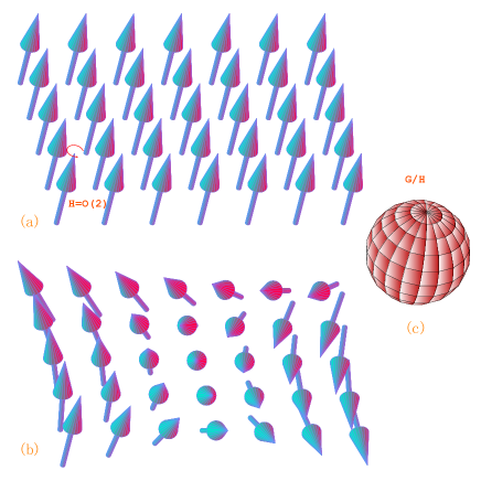
Figure 6: Spontaneous symmetry breaking in a Heisenberg ferromagnet. The ground state breaks the global rotational symmetry $G=O(3)$ (a). Collective fluctuations around this state, the Goldstone modes, are gapless (b). They are associated with the breaking of the symmetry $G/H=O(3)/O(2)\cong S^{2}$ (c).

The supermatrix $\sigma$ model bears a formal analogy to the Heisenberg ferromagnet. For the action (54), in the absence of the frequency term $\sim\omega\tilde{\omega}^{+}{\rm str}\Lambda Q$ it is invariant under the global gauge transformation: $Q\rightarrow U^{-1}QU$ where $U$ is a constant matrix belonging to the symmetry group $G$, which is $UOSP(2,2|4)$ for GOE systems and $U(1,1|2)$ for GUE systems. Each ‘ground state’, $Q_{0}$, solving the saddle point equation (55) breaks this continuous symmetry: in general, $U^{-1}Q_{0}U\neq Q_{0}$. Now, if we restore the frequency term, i.e., $\omega\tilde{\omega}^{+}\Lambda$ with $\tilde{\omega}\rightarrow 0$ in the matrix Green function ${\cal G}_{0}$ (cf. Eq. (55)), the system has a unique ‘ground state’ $\propto\Lambda$. In other words, the frequency (or the convergence-generating factor $\delta$ if $\tilde{\omega}=0$) term plays the role of the ‘external field’ and causes the spontaneous symmetry breaking.

Similar to Heisenberg ferromagnet this ‘ground state’ is invariant under the local gauge transformation: $Q_{0}\rightarrow U^{-1}({\bf r})Q_{0}U({\bf r})$ where $U({\bf r})\in H$ with $H=UOSP(2|2)\otimes UOSP(2|2)$ for GOE systems and $H=U(1|1)\otimes U(1|1)$ for GUE systems. Then, $T({\bf r})\in G/H$ describes the Goldstone modes and the action (69) describes the energy required for exciting low-lying modes. As expected $F[Q]|_{\tilde{\omega}^{+}=0}$ vanishes if $Q$ is homogeneous.

V Macroscopics of wave propagation in open media: general theory

In Ref. Tian07 , it was for the first time found at the full microscopic level that the diffusion coefficient in open media is position-dependent. However, very specific random media were studied in that work. Later, the microscopic approach used there was generalized to realistic random open media (see Sec. IV) and was used to systematically study transport of classical waves in these systems Tian08 ; Tian10 . Armed with the first-principles theory developed, it was found that the wave intensity correlation – a key characteristic of wave propagation – in open media is very different from that in infinite media Woelfle80a ; Woelfle80 ; Efetov83a . Specifically, such correlation function was found to obey Eq. (4) in the frequency ($\tilde{\omega}$) domain. Most strikingly, in Ref. Tian10 it was shown analytically and confirmed numerically that in the one-dimensional case, the static local (position-dependent) diffusion coefficient exhibits a novel scaling behavior. In this section, we shall establish the scaling theory in the more general case of slab open media in high dimensions.

From the technical viewpoint, the source of the difficulty can be seen in that even near the critical dimension the ordinary renormalization group scheme does not apply: one cannot replace the Boltzmann diffusion coefficient by the renormalized one obtained for infinite media because it does not account for effects arising from the openness of media such as resonances Lifshits79 ; Azbel83 ; Azbel83a . We therefore resort to calculating the wave intensity correlation by using the developed first-principles theory and then proceed to establish the macroscopic (or ‘hydrodynamic’, the term commonly adopted by condensed matter physicists) diffusion equation describing wave propagation. Restoring the source term and taking the corresponding derivatives of the partition function (53), we cast the correlation function (1) into a functional integral over the supermatrix field $Q({\bf r})$, i.e.,

$${\cal Y}({\bf r},{\bf r}^{\prime};\tilde{\omega})=\left(\frac{\pi\nu(\omega)}{8\omega}\right)^{2}\int D[Q]{\rm str}(A_{+}Q({\bf r})A_{-}Q({\bf r}^{\prime}))e^{-F[Q]}$$ (89)

for $\tilde{\omega}\ll\omega$, where $A_{\pm}=\sigma_{3}^{\rm fb}\otimes({\mathbbm{1}}\pm\sigma_{3}^{\rm ar})\otimes({\mathbbm{1}}-\sigma_{3}^{\rm tr})$. This expression is valid for both infinite media and finite-sized open media.

V.1 Wave propagation in infinite media

It is very illustrative to calculate Eq. (89) first for infinite media. In doing so, one may become familiar with perturbative calculations of the supersymmetric field theory, and appreciate – at the perturbative level – the main technical differences between infinite and finite-sized open media. We shall explain in detail the calculations for GOE systems and give the results for GUE systems directly.

V.1.1 Parametrization of the supermatrix $Q$

Notice the following identity,

$$T\equiv\left(\begin{array}[]{cc}T_{11}&T_{12}\\ T_{21}&T_{22}\\ \end{array}\right)^{\rm ar}=\left(\begin{array}[]{cc}T_{11}&0\\ 0&T_{22}\\ \end{array}\right)^{\rm ar}\left(\begin{array}[]{cc}1&T_{11}^{-1}T_{12}\\ T_{22}^{-1}T_{21}&1\\ \end{array}\right)^{\rm ar}\equiv\left(\begin{array}[]{cc}T_{11}&0\\ 0&T_{22}\\ \end{array}\right)^{\rm ar}(1+iW).$$ (98)

Upon inserting it into $Q$, we find

$$Q=(1+iW)^{-1}\Lambda(1+iW),\quad W=\left(\begin{array}[]{cc}0&B\\ kB^{\dagger}&0\\ \end{array}\right)^{\rm ar},$$ (101)

which is the so-called rational parametrization. The structure imposed on the $W$ matrix is fixed by two conditions. That is, $W$ anticommutes with $\Lambda$ and $Q^{\dagger}=KQK$ due to Eq. (35). The $4\times 4$ matrix $B$ can be parameterized as

$$B=\sum_{i=0}^{3}\left(\begin{array}[]{cc}a_{i}&i\sigma_{i}\\ \eta_{i}&ib_{i}\\ \end{array}\right)^{\rm fb}\otimes\sigma_{i}^{\rm tr},$$ (104)

where the entries of $a$’s and $b$’s ($\sigma$’s and $\eta$’s) are complex commuting (anticommuting) variables. They are not independent due to the constraint,

$$W^{\dagger}=-CW^{\rm T}C^{\rm T}$$ (105)

introduced by the condition (39), and the number of independent integral variables is reduced by one half. In Eq. (104), the subscript $i=0,3$ ($1,2$) stands for the diffuson (cooperon). An advantage of the rational parametrization is that the corresponding Jacobian (the so-called ‘Berezinian’) is unity. For perturbative calculations below, it is sufficient to take this as an exact mathematical theorem. We refer the reader interested in its proof to Ref. Efetov97 .

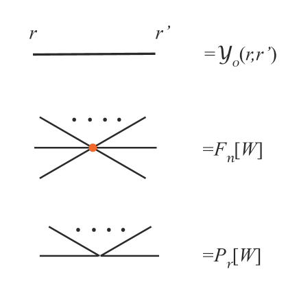
Figure 7: In the perturbation theory of the nonlinear supermatrix $\sigma$ model, each diagram is composed of the bare propagator (top) and the interaction vertexes (middle and bottom).

V.1.2 Wave interference corrections

For large $\tilde{\omega}$ we may expand Eq. (89) in terms of $W$. The action $F[Q]$ is given by $\sum_{n=1}^{\infty}F_{n}[W]$ with $F_{n}[W]\propto W^{2n}$. The pre-exponential factor leads to another $W$-expansion, $\sum_{r,s=0}^{\infty}{\rm str}(A_{+}P_{r}[W({\bf r})]A_{-}P_{s}[W({\bf r}^{\prime})])$, where $P_{r}[W]={\cal O}(W^{r})$. As a result,

$${\cal Y}({\bf r},{\bf r}^{\prime};\tilde{\omega})=\left(\frac{\pi\nu(\omega)}{8\omega}\right)^{2}\left\langle\sum_{r,s=0}^{\infty}{\rm str}(A_{+}P_{r}[W({\bf r})]A_{-}P_{s}[W({\bf r}^{\prime})])\sum_{m=0}^{\infty}\frac{1}{m!}\left(\sum_{n=2}^{\infty}F_{n}[W]\right)^{m}\right\rangle_{0},$$ (106)

where the average is defined as $\langle\cdot\rangle_{0}\equiv\int D[W](\cdot)\exp(-F_{1}[W])$, with $F_{1}[W]=-\frac{\pi\nu}{2}\int d{\bf r}{\rm str}(D_{0}(\nabla iW)^{2}-i\tilde{\omega}(iW)^{2})$. This perturbative expansion describes the interaction between diffusons and cooperons, and each term can be calculated by using Wick’s theorem with the help of the following contraction rules,

$$4\pi\nu\langle W({\bf r})MW({\bf r}^{\prime})\rangle_{0} = {\cal Y}_{0}({\bf r},{\bf r}^{\prime};\tilde{\omega})\left[({\rm str}M+{\bar{M}})-\Lambda({\rm str}(M\Lambda)+{\bar{M}}\Lambda)\right],$$

$$4\pi\nu\langle{\rm str}(W({\bf r})M){\rm str}(W({\bf r}^{\prime})M^{\prime})\rangle_{0} = {\cal Y}_{0}({\bf r},{\bf r}^{\prime};\tilde{\omega}){\rm str}((M-{\bar{M}})(M^{\prime}-\Lambda M^{\prime}\Lambda)),$$ (107)

with $\bar{M}=KCM^{\rm T}C^{\rm T}K$. The propagator, ${\cal Y}_{0}({\bf r},{\bf r}^{\prime};\tilde{\omega})$, solves the normal diffusion equation,

$$(-i{\tilde{\omega}}-D_{0}\nabla^{2}){\cal Y}_{0}({\bf r},{\bf r}^{\prime};{\tilde{\omega}})=\delta({\bf r}-{\bf r}^{\prime}),$$ (108)

which, importantly, is translationally invariant, i.e., ${\cal Y}_{0}({\bf r},{\bf r}^{\prime};\tilde{\omega})={\cal Y}_{0}({\bf r}-{\bf r}^{\prime},0;\tilde{\omega})$. The contraction rules can be proved straightforwardly by using the parametrization (101) and (104). With all the contractions made, each term in the expansion (106) can be represented by a diagram composed of the (bare) propagator ${\cal Y}_{0}({\bf r},{\bf r}^{\prime};\tilde{\omega})$ (representing the corresponding contraction), and the ‘interaction’ vertices $F_{n\geq 2}[W]$ and $P_{r}[W]$ (Fig. 7). The diagram is either reducible or irreducible, depending on whether it may be divided into two disconnected subdiagrams by cutting some bare propagator.

Let us start from the lowest order term (${\cal O}(W^{2})$) in Eq. (106), i.e.,

$$-\left(\frac{\pi\nu(\omega)}{4\omega}\right)^{2}\int D[W]e^{-F_{1}[W]}{\rm str}(A_{+}iW({\bf r})A_{-}iW({\bf r}^{\prime})).$$ (109)

With the help of the contraction rules (V.1.2) we find that at this perturbation level, the correlator ${\cal Y}({\bf r},{\bf r}^{\prime};\tilde{\omega})$ is identical to the bare correlator ${\cal Y}_{0}({\bf r},{\bf r}^{\prime};\tilde{\omega})$, which excludes all wave interference effects. The subleading term is ${\cal O}(W^{4})$ with all the irreducible diagrams given in Fig. 8. (Notice that $F_{n}[W]\propto W^{2n}={\cal O}(W^{2(n-1)})$ for $F_{1}[W]={\cal O}(1)$.) These terms contribute wave interference corrections to the bare correlator. More precisely, at this perturbation level the correlator is (see Appendix E for details)

$${\cal Y}_{0}({\bf r},{\bf r}^{\prime};\tilde{\omega})+\delta{\cal Y}_{1}({\bf r},{\bf r}^{\prime};\tilde{\omega})$$ (110)

$$= -\left(\frac{\pi\nu(\omega)}{4\omega}\right)^{2}\int D[W]e^{-F_{1}[W]}{\rm str}(A_{+}iW({\bf r})A_{-}iW({\bf r}^{\prime}))\left(1+\frac{\pi\nu}{2}\int d{\bf r}_{1}\delta D^{(1)}(\tilde{\omega}){\rm str}(\nabla iW({\bf r}_{1}))^{2}\right),$$

where

$$\delta D^{(1)}({\tilde{\omega}})=-\frac{D_{0}}{\pi\nu}{\cal Y}_{0}(0,0;{\tilde{\omega}}).$$ (111)

By re-exponentiating the last factor (which is equivalent to summing up all the reducible diagrams with the one-loop vertex) we rewrite Eq. (110) as

$${\cal Y}({\bf r},{\bf r}^{\prime};\tilde{\omega})\approx-\left(\frac{\pi\nu(\omega)}{4\omega}\right)^{2}\int D[W]e^{\frac{\pi\nu}{2}\int d{\bf r}_{1}{\rm str}(D(\tilde{\omega})(\nabla iW)^{2}-i\tilde{\omega}(iW)^{2})}{\rm str}(A_{+}iW({\bf r})A_{-}iW({\bf r}^{\prime})).$$ (112)

Comparing the Gaussian wight with that of Eq. (109), we find that wave interference renormalizes the bare diffusion coefficient, i.e., $D_{0}\rightarrow D(\tilde{\omega})=D_{0}+\delta D^{(1)}(\tilde{\omega})$, and $\delta D^{(1)}(\tilde{\omega})$ is the well-known weak localization correction Woelfle80a ; Woelfle80 ; Larkin79 namely Eq. (3). The correlator (112) solves the macroscopic equation (2).

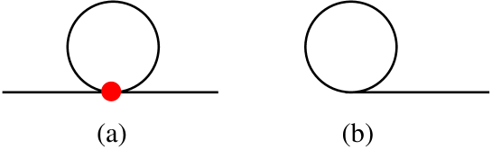
Figure 8: Diagrams give the leading order wave interference correction to the Boltzmann diffusion constant.

Importantly, the diagram (b) in Fig. 8 guarantees that the wave interference correction to the bare propagator ${\cal Y}_{0}$ vanishes when ${\cal Y}_{0}$ is homogeneous in space Tian08 (see also Appendix E for the proof). In general, the roles of the expansion of the pre-exponential factor are to conform with an exact Ward identity reflecting the energy conservation law,

$${\cal Y}({\bf r},{\bf r}^{\prime};{\tilde{\omega}})\stackrel{{\scriptstyle\nabla{\cal Y}=0}}{{=}}\frac{1}{-i\tilde{\omega}}.$$ (113)

This must be respected at all levels of the perturbation. In the diagrammatic perturbation theory, conforming to this identity necessitates the introduction of the well-known Hikami box Hikami81 .

For GUE systems the leading order weak localization correction (111) vanishes. This certainly does not imply the absence of interference effects in the weak (not strong) localization regime. The point is that wave interference (see Fig. 11 for example) can be much more complicated and quantitatively they give higher order weak localization corrections. It must be emphasized that these higher order corrections cannot be obtained by calculating reducible diagrams with one-loop vertex.

Let us now consider the terms $\sim{\cal O}(W^{6})$. The irreducible diagrams of this order are given in Fig. 9. (Recall that $F_{2}[W]={\cal O}(W^{2})$ and $F_{3}[W]={\cal O}(W^{4})$.) The derivation is similar to that of deriving $\delta D^{(1)}(\tilde{\omega})$ but is much more complicated. By using the contraction rules (V.1.2) one may show that for GOE systems the correction given by Fig. 9 (denoted as $\delta{\cal Y}_{2}({\bf r},{\bf r}^{\prime};\tilde{\omega})$) vanish, i.e.,

$$\delta D^{(2)}(\tilde{\omega})=0,\,{\rm for\,GOE}.$$ (114)

For GUE systems here we will emphasize the key points and only give the final result Tian12a . First of all, Fig. 9 (d) - (g) again conforms to the Ward identity (113). Secondly, $\delta{\cal Y}_{2}({\bf r},{\bf r}^{\prime};\tilde{\omega})$ consists of two contributions, i.e.,

$$\delta{\cal Y}_{2}({\bf r},{\bf r}^{\prime};\tilde{\omega}) = -\left(\frac{\pi\nu(\omega)}{4\omega}\right)^{2}\frac{\pi\nu D_{0}}{2}\int D[W]e^{-F_{1}[W]}{\rm str}(A_{+}iW({\bf r})A_{-}iW({\bf r}^{\prime}))\int d{\bf r}_{1}\!\!\int d{\bf r}_{2}{\rm str}\left(\nabla^{\alpha}iW({\bf r}_{1})\nabla^{\beta}iW({\bf r}_{2})\right)$$ (115)

$$\times\left[\frac{1}{2}\left(\frac{{\cal Y}_{0}({\bf r}_{1},{\bf r}_{2};{\tilde{\omega}})}{\pi\nu}\right)^{2}\delta({\bf r}_{1}-{\bf r}_{2})\delta_{\alpha\beta}+D_{0}\nabla^{\alpha}\nabla^{\beta}{\cal Y}_{0}({\bf r}_{1},{\bf r}_{2};{\tilde{\omega}})\left(\frac{{\cal Y}_{0}({\bf r}_{1},{\bf r}_{2};{\tilde{\omega}})}{\pi\nu}\right)^{2}\right].$$

The first contribution leads to a wave interference correction to $D_{0}$ which is local in space thanks to the factor $\delta({\bf r}_{1}-{\bf r}_{2})$, while the second one to a correction non-local in space. The non-locality arises from diagrams such as Fig. 9 (a). Because the system is isotropic, the crossing terms, $\sim\nabla^{\alpha}\nabla^{\beta},\,\alpha\neq\beta$, do not contribute upon integrating out the space coordinates. As a result, Eq. (115) is simplified to

$$\delta{\cal Y}_{2}({\bf r},{\bf r}^{\prime};\tilde{\omega}) = -\left(\frac{\pi\nu(\omega)}{4\omega}\right)^{2}\frac{\pi\nu D_{0}}{2}\int D[W]e^{-F_{1}[W]}{\rm str}(A_{+}iW({\bf r})A_{-}iW({\bf r}^{\prime}))\int d{\bf r}_{1}\!\!\int d{\bf r}_{2}{\rm str}\nabla iW({\bf r}_{1})\cdot\nabla iW({\bf r}_{2})$$ (116)

$$\times\left[\frac{1}{2}\left(\frac{{\cal Y}_{0}({\bf r}_{1},{\bf r}_{2};{\tilde{\omega}})}{\pi\nu}\right)^{2}\delta({\bf r}_{1}-{\bf r}_{2})+\frac{D_{0}}{d}\nabla^{2}{\cal Y}_{0}({\bf r}_{1},{\bf r}_{2};{\tilde{\omega}})\left(\frac{{\cal Y}_{0}({\bf r}_{1},{\bf r}_{2};{\tilde{\omega}})}{\pi\nu}\right)^{2}\right].$$

In the hydrodynamic limit the spatial and time derivatives in the macroscopic equation are decoupled. Taking this into account, Eq. (116) reduces to

$$\delta{\cal Y}_{2}({\bf r},{\bf r}^{\prime};\tilde{\omega}) \rightarrow -\left(\frac{\pi\nu(\omega)}{4\omega}\right)^{2}\frac{\pi\nu D_{0}}{2}\int D[W]e^{-F_{1}[W]}{\rm str}(A_{+}iW({\bf r})A_{-}iW({\bf r}^{\prime}))\int d{\bf r}_{1}\!\!\int d{\bf r}_{2}{\rm str}\nabla iW({\bf r}_{1})\cdot\nabla iW({\bf r}_{2})$$ (117)

$$\times\left[\frac{1}{2}\left(\frac{{\cal Y}_{0}({\bf r}_{1},{\bf r}_{2};{\tilde{\omega}})}{\pi\nu}\right)^{2}\delta({\bf r}_{1}-{\bf r}_{2})+\frac{1}{d}(D_{0}\nabla^{2}+i\tilde{\omega}){\cal Y}_{0}({\bf r}_{1},{\bf r}_{2};{\tilde{\omega}})\left(\frac{{\cal Y}_{0}({\bf r}_{1},{\bf r}_{2};{\tilde{\omega}})}{\pi\nu}\right)^{2}\right]$$

$$= -\left(\frac{\pi\nu(\omega)}{4\omega}\right)^{2}\int D[W]e^{-F_{1}[W]}{\rm str}(A_{+}iW({\bf r})A_{-}iW({\bf r}^{\prime}))\frac{\pi\nu}{2}\int d{\bf r}_{1}\delta D^{(2)}(\tilde{\omega}){\rm str}(\nabla iW({\bf r}_{1}))^{2},$$

where the wave interference correction to $D_{0}$ is local, read

$$\delta D^{(2)}(\tilde{\omega})=\left(\frac{1}{2}-\frac{1}{d}\right)D_{0}\left(\frac{{\cal Y}_{0}(0,0;{\tilde{\omega}})}{\pi\nu}\right)^{2},\,{\rm for\,GUE}.$$ (118)

At this perturbation level, the correlation function is ${\cal Y}={\cal Y}_{0}+\delta{\cal Y}_{1}+\delta{\cal Y}_{2}$ which solves the macroscopic diffusion equation (2), with the dynamic diffusion coefficient replaced by $D(\tilde{\omega})=D_{0}+\delta D^{(1)}(\tilde{\omega})+\delta D^{(2)}(\tilde{\omega})$. At the higher order perturbation level, Eq. (2) remains valid with $D(\tilde{\omega})$ including corresponding higher order corrections.

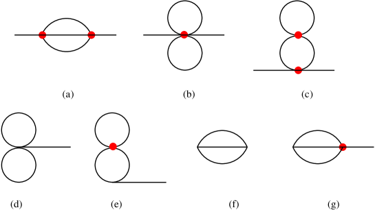
Figure 9: Diagrams give the subleading order wave interference correction to the Boltzmann diffusion constant.

Notice that there are two opposite contributions to $\delta D^{(2)}(\tilde{\omega})$, accounting for the factor $\frac{1}{2}$ and $-\frac{1}{d}$, respectively. The wave interference picture underlying the former Altshuler98 ; Tian04 (see also Fig. 11 below) may be related to the interesting phenomenon of coherent forward scattering Mueller12 . Importantly, the factor $(\frac{1}{2}-\frac{1}{d})$ ensures the renormalizability: approaching two dimensions (from below), this infinitesimal factor cancels one logarithmically diverging factor arising from ${\cal Y}_{0}(0,0;{\tilde{\omega}})$ and makes the two-loop correction diverge only logarithmically. Upon making the analytic continuation from dimensions below two to above, we find from Eqs. (111), (114) and (118) the well-known scaling equation for the dimensionless Thouless conductance $g(L_{\tilde{\omega}})=\pi\nu D_{0}L_{\tilde{\omega}}^{d-2}/\Omega_{d}$ with $L_{\tilde{\omega}}=\sqrt{D_{0}/{\tilde{\omega}}}$ and $\Omega_{d}$ the volume of $d$-dimensional unit sphere, i.e.,

$$\frac{d\ln g}{d\ln L_{\tilde{\omega}}}=\bigg{\{}\begin{array}[]{c}d-2-\frac{1}{g}+{\cal O}(\frac{1}{g^{3}}),\quad{\rm for\,GOE},\\ d-2-\frac{1}{2g^{2}}+{\cal O}(\frac{1}{g^{3}}),\quad{\rm for\,GUE}\end{array}$$ (121)

near the critical dimension Efetov97 ; Anderson79 .

We wish to make some remarks here. (i) In the presence of magneto-optical effects the one-loop weak localization may be fully suppressed. In this case, the critical theory is described by the second equation (121). This overcomes the notable difficulty of the self-consistent diagrammatic approach Woelfle80a ; Woelfle80 which cannot be used to study localization of GUE systems. This is a simple example showing the field theoretic approach to be a powerful technique in studies of localization in magneto-optical systems. (ii) The criticality described by the scaling equation is quantitatively accurate in $2+\epsilon$ ($\epsilon\equiv d-2$ which should not be confused with the dielectric constant) dimensions since the critical point $g^{*}={\cal O}(\epsilon^{-1})\gg 1$. One may extrapolate the results into three dimensions by setting $\epsilon=1$. In particular, we find that the Ioffe-Regel criterion is also valid for GUE systems. This may guide experimental search of light localization in magneto-optical systems. (iii) In combination with Eq. (64) this criterion predicts that there is a mobility edge separating low-frequency extended states and high-frequency localized states. (iv) In low dimensions ($d<2$), the dimensionless conductance decreases as the frequency $\tilde{\omega}$ is lowered. In this case, all the higher order irreducible diagrams are important. Similar to the above analysis, these give local corrections to the Boltzmann constant. This implies the validity of the macroscopic equation (2) for low $\tilde{\omega}$. However, obtaining the explicit form of $D(\tilde{\omega})$ is beyond the perturbation scheme and one must resort to non-perturbative treatments of the supersymmetric nonlinear $\sigma$ model. This indeed has been done by Efetov and Larkin Efetov83a in the Q$1$D case. (v) According to the exact (non-perturbative) solution given in Ref. Efetov83a , in Q$1$D the localization length $\xi\sim\nu(\omega)D_{0}(\omega)$. This implies that the localization length diverges as $\omega^{-2}$ in the limit $\omega\rightarrow 0$. Notice that this scaling law is universal (but the coefficient not): it is the same for both GOE and GUE systems. (vi) In two dimension the localization length diverges exponentially in the low-frequency limit. The behavior depends on system’s symmetry: $\ln\xi\sim\omega^{-2}$ for GOE systems and $\ln\xi\sim\omega^{-4}$ for GUE systems. The latter results from the infinitesimal factor of $(\frac{1}{2}-\frac{1}{d})$.

V.2 Wave propagation in open media

We now consider the case of open media and investigate how the results above are modified. Let us begin with a pictorial illustration in terms of the supermatrix field of the main difference between infinite and finite-sized open media. We then substantiate the picture with explicit calculations of the wave intensity correlator.

V.2.1 A pictorial illustration

For simplicity let us consider the discrete space lattice (with the lattice constant set to unity). In this case, the nonlinear $\sigma$ model action (69) is written as

$$F[Q]=-\nu D_{0}\sum_{\langle ij\rangle}{\rm str}Q_{i}Q_{j}+\frac{\pi\nu i\tilde{\omega}^{+}}{4}\sum_{i}{\rm str}\Lambda Q_{i},\quad Q_{i}^{2}=1,$$ (122)

where $i$ stands for the lattice site and the summation is over all the nearest neighbors, $\langle ij\rangle$. Comparing Eqs. (88) and (122) we find that these two models bear a firm analogy summarized in Table 1. Notice that the supermatrix structure of $Q$ as well as the supertrace operation is irrelevant for present discussions.

Identifying this analogy, we may translate some well-known facts regarding the ferromagnetic system Chaikin to the present supermatrix $\sigma$ model. For the ferromagnetic system, if the temperature is sufficiently low, spins tend to align in parallel as a result of the so-called spontaneous symmetry breaking. In the presence of the external magnetic field ${\bf h}$ they are all parallel to the magnetic field. Such an ordered phase is the ferromagnetic phase accompanied by long-ranged order. Namely, the spatial correlation of two spins does not vanish when their distance approaches infinity. If the temperature is sufficiently high, spins strongly fluctuate in space and the average magnetization is zero. Such a disordered phase is the paramagnetic phase. In this phase, a nonvanishing average magnetization can be triggered only by an external magnetic field. Unlike the ferromagnetic phase, the spin-spin correlation decays exponentially when the distance exceeds the correlation length. At some critical temperature a transition from the ferromagnetic to paramagnetic phase occurs, accompanied by large spin fluctuations.

This scenario has an analogy in the supersymmetric nonlinear $\sigma$ model. As mentioned above, the supermatrix $Q$ field mimics the spin. In high dimensions ($d>2$), the metallic phase – the ‘ferromagnetic phase’ – is formed, if disorders are weak enough (large $\nu D_{0}$), in which the ‘spins’ $Q$ tend to align. In the presence of $\tilde{\omega}$ they all point towards ‘north pole’, $\Lambda$. ‘Spin’ fluctuations in space characterize diffusive modes (diffuson and cooperon) and their interactions, and long-range order is manifested in the spatial extension of wave functions. In this ordered phase, ‘spin’ fluctuations are weak characterizing a metal suffering weak localization. If disorder is strong enough (small coupling constant $g_{0}$) or in low dimensions ($d\leq 2$), the system is in the insulator phase – the ‘paramagnetic phase’ – where the ‘spin’ $Q$ fluctuates strongly in space. In this disordered phase, the correlation of the ‘spin’ $Q$ falls exponentially at large distances with the ‘correlation length’ being the localization length $\xi$. This is manifested in the exponential localization of wave functions. As we have seen from the scaling theory (121), in dimension $d>2$, a metal-insulator transition is triggered by lowering the coupling constant $g_{0}$: this is the analogy of (thermodynamic) ferromagnetic-paramagnetic transition. We wish to point out that the above supermatrix - spin analogy should not be carried too far: notably, the supermatrix $Q$ field does not play the role of the order parameter in the Anderson transition Efetov97 . In fact, the average ‘magnetization’, $k\Lambda Q$, does not vanish in both phases. Physically, this is so because the density of states is not critical in the Anderson transition.

(For simplicity, below we focus on the static case, i.e., ${\tilde{\omega}}=0$.) Open media (without internal reflection) differ from infinite media in that outside the medium, the ‘spin’ $Q$ is fixed, pointing towards ‘north pole’ $\Lambda$ (the red arrows in Fig. 10). Due to the ‘ferromagnetic’ coupling, near the boundary the ‘spin’ $Q$ tends to align with $\Lambda$. As the distance to the interface increases, the $Q$-field fluctuations becomes stronger (Fig. 10). Since such fluctuations characterize wave interference, the interference strength increases as waves propagate from the interface to the sample center. Since homogeneous wave interference effects lead to a spatially homogeneous diffusion coefficient, $D(\tilde{\omega})$, in infinite media, one may naturally expect that in open media a local diffusion coefficient $D({\bf r};\tilde{\omega})$ results.

Table 1: Ferromagnet-supermatrix $\sigma$ model analogy

	Heisenberg ferromagnet	supermatrix $\sigma$ model
system’s energy	$\mathscr{H}[{\bf S}]$	$F[Q]$
spin	$S_{i}$	$Q_{i}$
constraint	$S_{i}^{2}=1$	$Q_{i}^{2}=1$
coupling constant	$J$	$\nu D_{0}$
magnetic field	${\bf h}$	$-\frac{\pi\nu i\tilde{\omega}^{+}}{4}\Lambda$
ordered phase	ferromagnet	metal
disordered phase	paramagnet	insulator

V.2.2 Local diffusion equation and single parameter scaling of $D({\bf r};\tilde{\omega})$

Let us first consider the boundary constraint. The role of the second term of Eq. (86) is to align $Q$ to $\Lambda$. Indeed, if we ignore for the moment the first term and substitute into it the parametrization (101), we find $W({\bf r}\in C)=0$, i.e., $Q({\bf r}\in C)=\Lambda$. For $\zeta$ much smaller than the inverse of the typical value of the boundary derivative $Q\nabla_{{\bf n}({\bf r})}Q$ which is $\sim{\cal O}({\rm min}(L,\xi))$, we may keep the leading order expansion in $W$, obtaining

$$(\zeta\nabla_{{\bf n}({\bf r})}-1)W=0.$$ (123)

This implies that $W$ – if extended to the air from the random medium – would decay exponentially for distances to the interface much larger than $\zeta$. In other words, the Goldenstone modes tend to penetrate into the air for a distance $\sim\zeta$. This translates the canonical physical interpretation of the extrapolation length into the field theoretical language. More precisely, for $\zeta\ll{\rm min}(\xi,L)$, the boundary constraint (86) is simplified to

$$Q|_{{\bf r}\in C^{\prime}}=\Lambda,$$ (124)

where $C^{\prime}$ is the trapping plane outside the medium and of a distance $\zeta$ to the interface $C$. Then, effect of the simplified boundary condition (124) is to enlarge the size of the medium by a thickness of $\zeta$, which is well known for diffusive media Niuwenhuizen .

It should be emphasized that the boundary condition (124) also applies to the localized system, provided the condition $\zeta\ll\xi$ is met. This implies that the common wisdom Niuwenhuizen for a diffusive (slab) sample – that its effective thickness is larger than its actual thickness by $2\zeta$ – can be extended even to a localized sample. Most importantly, such common wisdom should not be carried to the case of strong internal reflection where $\zeta\gtrsim{\rm min}(\xi,L)$. In this case, the perturbative expansion for Eq. (86) ceases to work and Eq. (124) breaks down.

In this review, we are interested in the simplest case in which internal reflection is absent. In this case, $\zeta\sim l$ is much smaller than any other macroscopic scale. For this reason, we may ignore the slight difference of $2\zeta$ between the effective and actual thickness of the sample, and from now on set $C^{\prime}=C$. We then repeat the procedures of Sec. V.1 for deriving Eq. (2). A summary of the essential differences from Sec. V.1 in the final results is as follows: (i) the propagator ${\cal Y}_{0}$ is no longer translationally invariant, i.e., ${\cal Y}_{0}({\bf r},{\bf r}^{\prime};\tilde{\omega})\neq{\cal Y}_{0}({\bf r}-{\bf r}^{\prime},0;\tilde{\omega})$. The translational symmetry is broken by the boundary condition: ${\cal Y}_{0}({\bf r}\in C,{\bf r}^{\prime};\tilde{\omega})=0$ which is a result of Eq. (124). (ii) Because of (i), the probability density ${\cal Y}_{0}({\bf r},{\bf r};\tilde{\omega})$ is no longer homogeneous, but rather, depends on the position ${\bf r}$ explicitly. (iii) Up to two loops the weak localization correction is

$$\delta D({\bf r};\tilde{\omega})=D_{0}\left[-\frac{{\cal Y}_{0}({\bf r},{\bf r};\tilde{\omega})}{\pi\nu}+C\left(\frac{1}{2}-\frac{1}{d}\right)\left(\frac{{\cal Y}_{0}({\bf r},{\bf r};{\tilde{\omega}})}{\pi\nu}\right)^{2}\right].$$ (125)

which as a result of (ii), is no longer homogeneous. Here, $C$ is zero (unity) for GOE (GUE) systems. The first term was also obtained in Ref. Skipetrov08 by the refined diagrammatic perturbation theory. (iv) Remarkably, the correlator ${\cal Y}$ solves Eq. (4) instead of Eq. (2), with the local diffusion coefficient given by

$$D({\bf r},{\tilde{\omega}})=D_{0}+\delta D({\bf r};{\tilde{\omega}}).$$ (126)

For ${\bf r}$ being at the sample center, sending $L$ to infinity (so that effects arising from interfaces do not play any role), we recover ordinary single parameter scaling equation (121) from Eq. (125) for $d$ near the critical dimension.

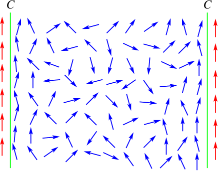
Figure 10: The supermatrix $Q$ and the supersymmetric nonlinear $\sigma$ model mimic the spin and the Heisenberg model of ferromagnetism, respectively. The ‘spin’ $Q$ is frozen on the transparent interface (red), and fluctuations increase inside the medium (blue).

Most strikingly, Eq. (125) shows that the local diffusion coefficient depends on ${\bf r}$ (as well as $\tilde{\omega}$) via the scaling factor $\lambda({\bf r};{\tilde{\omega}})=(\pi\nu)^{-1}{\cal Y}_{0}({\bf r},{\bf r};\tilde{\omega})$. In fact, such a dependence persists to higher orders. This shows that the local diffusion coefficient exhibits novel single parameter scaling, i.e.,

$$\frac{D({\bf r};{\tilde{\omega}})}{D_{0}}=D_{\infty}(\lambda({\bf r};{\tilde{\omega}})),$$ (127)

where $D_{\infty}(\lambda)$ is some scaling function depending on both symmetries and dimensions. It is important that the novel scaling (127) is valid also for large $\lambda$, the non-perturbative regime. This scaling, as we will see in the next section, is the key component in the description of macroscopic wave transport through one-dimensional open localized media. It is missed by the SCLD model Lagendijk00 . We emphasize that the inability of the SCLD model to capture this scaling is intrinsic to the phenomenological assumption of one-loop self-consistency in open media, but not to the VW theory Woelfle80a ; Woelfle80 which is formulated for infinite systems. Indeed, if we set ${\bf r}$ to the sample center and send $L$ to infinity, the scaling factor diverges as $\ln{\tilde{\omega}}$ (${\tilde{\omega}}^{-1/2}$) in two (one) dimensions, and the VW theory captures these infrared divergences and was designed for the purpose of (partly) summing up these divergences.

The diffusion coefficient (126) and the local diffusion equation (4) have important implications. (For media without internal reflection,) localization effects are absent on the interface, i.e., $D({\bf r}\in C;\tilde{\omega})=D_{0}$, which is robust against wave interference. In particular, there is no boundary layer which scales in the same way as the diffusion constant in an infinite medium, as was assumed by the earlier phenomenological model Berkovits87 . As indicated by Eq. (125), this arises from the inhomogeneity of wave interference effects in open media. Near the interface, wave interference characterized by ${\cal Y}_{0}({\bf r},{\bf r};\tilde{\omega})$ is largely diminished due to wave energy leakage through the interface.

V.2.3 Origin of the novel scaling

It should be stressed that the novel scaling (127) applies to the local diffusion coefficient and therefore describes the unconventional hydrodynamic behavior of wave propagation in open media. It is fundamentally different from the ordinary single parameter scaling theory of the Thouless conductance Anderson79 , which provides no information on how wave energies flow from one point to the other inside the medium. As we will see in Sec. VI.3, the former leads to the latter and contains significantly more information on wave transport. Now, let us discuss the origin of the novel scaling. First of all, optical paths may self-intersect, forming a loop. It is well known that because of the time-reversal symmetry two optical paths may counterpropagate along this loop and interfere constructively with each other, leading to the (one-loop) weak localization correction Altshuler83 ; Bergmann84 homogeneous in space (Fig. 11, upper left). In the presence of open interfaces, the interference picture is modified. That is, wave energies leak out the system through the interfaces (Fig. 11, upper right) and as such, at time $t$ the probability for a path to return to the vicinity (of size $\sim{\mathchar 22\relax\mkern-10.0mu\lambda}^{d-1}dt$) of its departure point explicitly depends on the departure point ${\bf r}$: the returning probability is $\sim{\cal Y}_{0}({\bf r},{\bf r}^{\prime}={\bf r};t){\mathchar 22\relax\mkern-10.0mu\lambda}^{d-1}dt$ and increases as ${\bf r}$ moves into the medium. Here, ${\cal Y}_{0}({\bf r},{\bf r}^{\prime};t)$ is the inverse Fourier transform of ${\cal Y}_{0}({\bf r},{\bf r}^{\prime};{\tilde{\omega}})$. Since wave interference enhances the backscattering probability, the diffusion coefficient is suppressed by an amount

$$\frac{\delta D^{(1)}({\bf r};{\tilde{\omega}})}{D_{0}}\sim-{\mathchar 22\relax\mkern-10.0mu\lambda}^{d-1}\int dte^{i{\tilde{\omega}}t}{\cal Y}_{0}({\bf r},{\bf r};t)\sim-\lambda({\bf r};{\tilde{\omega}}).$$ (128)

As waves penetrate deeper inside the medium, more complicated wave interference effects take place. For example, optical paths tend to return to the vicinity of its departure point more (say $n$) times (e.g., Fig. 11, lower panel) Altshuler98 ; Tian04 , with a probability $\sim({\mathchar 22\relax\mkern-10.0mu\lambda}^{d-1})^{n}\int_{t_{1}>t_{2}>\cdots>t_{n-1}}dt_{1}dt_{2}\cdots dt_{n-1}{\cal Y}_{0}({\bf r},{\bf r};t-t_{1}){\cal Y}_{0}({\bf r},{\bf r};t_{1}-t_{2})\cdots{\cal Y}_{0}({\bf r},{\bf r};t_{n-1})$. Two paths taking these loops as their routes pass the $n$ loops in different orders. Having (almost) the same phases, they also interfere constructively. This results in a higher order wave interference correction,

$$\frac{\delta D^{(n)}({\bf r};{\tilde{\omega}})}{D_{0}} \sim ({\mathchar 22\relax\mkern-10.0mu\lambda}^{d-1})^{n}\int dte^{i{\tilde{\omega}}t}\int_{t_{1}>t_{2}>\cdots>t_{n-1}}dt_{1}dt_{2}\cdots dt_{n-1}{\cal Y}_{0}({\bf r},{\bf r};t-t_{1}){\cal Y}_{0}({\bf r},{\bf r};t_{1}-t_{2})\cdots{\cal Y}_{0}({\bf r},{\bf r};t_{n-1})$$ (129)

$$\sim \left(\lambda({\bf r};{\tilde{\omega}})\right)^{n}.$$

Thus, the position ${\bf r}$ enters into all the wave interference corrections via the position-dependent return probability, which justifies the novel scaling. It is important that for $n\geq 2$, the two optical paths, though passing the loops in different orders, may propagate along every loop in the same direction (clockwise or anticlockwise). Such constructive interference picture does not require time-reversal symmetry, and is key to establishing both the local diffusion and novel scaling in GUE systems.

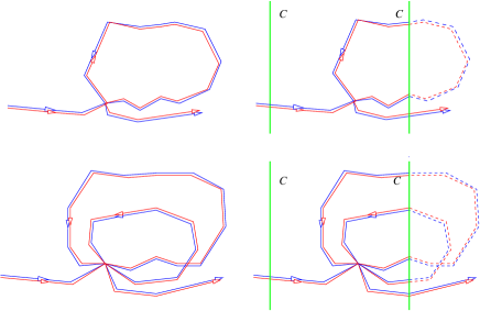
Figure 11: Left: examples of interference picture in infinite media. Right: in open media, wave interference is suppressed because wave energies leak out of the system (dashed line). Upper: interference picture underlying one-loop weak localization. Lower: examples of more complicated interference picture. The green line, $C$, stands for the air-medium interface.

V.2.4 Unconventional Ohm’s law

The existence of the local diffusion coefficient leads to an interesting phenomenon – the unconventional Ohm’s law in the steady state ($\tilde{\omega}=0$). Indeed, if the transverse plane of the slab is infinite, the local diffusion coefficient is homogeneous in the transverse direction. As a result, $D({\bf r};\tilde{\omega}=0)=D(x;\tilde{\omega}=0)\equiv D(x)$, where $x$ is the longitudinal coordinate $x$. In the steady states, the system may sustain a uniform macroscopic current in the longitudinal direction, $j$, going through the slab. An intensity profile across the sample, $I(x)$, which is uniform in the transverse direction is thereby built up. Eq. (4) gives the local Fick’s law,

$$j=-D(x)\partial_{x}I(x),$$ (130)

according to which the intensity bias across the sample is $I(L)-I(0)=-j\int_{0}^{L}\frac{dx}{D(x)}$. Since the ensemble-averaged transmission $\langle T(L)\rangle\propto j/(I(L)-I(0))$, we find

$$\langle T(L)\rangle^{-1}\sim\int_{0}^{L}\frac{dx}{D(x)}.$$ (131)

It suggests that the total resistance of the system, $\langle T(L)\rangle^{-1}$, is the integration of the infinitesimal resistance, $\frac{dx}{D(x)}$. In this sense, it is similar to the familiar Ohm’s law. However, it should be emphasized that in sharp contrast to the ordinary Ohm’s law, the resistivity $D^{-1}(x)$ is no longer inhomogeneous in space. In particular, we will see in the next section that for localized samples $D^{-1}(x)$ may increase by many orders of magnitude as the position changes from the interface to the midpoint, and it is the dramatic enhancement of $D^{-1}(x)$ near the sample center that leads the system to exhibit a global localization behavior namely the exponential decay of the average transmission in the sample length. (For diffusive samples, such position-dependence is weak and does not lead to any interesting phenomena other than the scaling $\langle T(L)\rangle\sim 1/L$.) For this reason, we term Eq. (131) ‘unconventional Ohm’s law’. Such law was first conjectured in Ref. Lagendijk00 . The microscopic justification of Eq. (4) puts this important conjecture on a firm level.

VI Local diffusion in one dimension

In the one-dimensional case, the asymptotic behavior of the scaling function $D_{\infty}(\lambda)$ at large $\lambda$ has been found analytically Tian10 , which will be discussed in this section. In this case, the macroscopic diffusion equation (4) is simplified to

$$(-i\tilde{\omega}-\partial_{x}D(x;\tilde{\omega})\partial_{x}){\cal Y}(x,x^{\prime};\tilde{\omega})=\delta(x-x^{\prime}),$$ (132)

which is implemented with the boundary condition,

$${\cal Y}(x,x^{\prime};\tilde{\omega})|_{x=0\,{\rm or}\,L}=0$$ (133)

due to transparent interfaces. Single parameter scaling (127) is simplified to

$$\frac{D(x;{\tilde{\omega}})}{D_{0}}=D_{\infty}(\lambda(x;{\tilde{\omega}})),$$ (134)

and the scaling factor to

$$\lambda(x;\tilde{\omega})\equiv\frac{{\cal Y}_{0}(x,x;\tilde{\omega})}{\pi\nu}=\frac{L}{\xi}\frac{\cosh\sqrt{\omega^{*}}-\cosh(\sqrt{\omega^{*}}(1-2x/L))}{2\sqrt{\omega^{*}}\sinh\sqrt{\omega^{*}}},$$ (135)

with ${\omega^{*}}\equiv-i\tilde{\omega}L^{2}/D_{0}$. Throughout this section the ‘effective’ local density of states is the product of the local density of states and the cross-sectional area of Q$1$D samples, $S$, and we denote it as $\nu$ also in order to simplify notations. The localization length $\xi\sim\nu D_{0}$ Efetov83a . We emphasize that Eqs. (132)-(135) are valid for both GOE and GUE systems.

Below, we will study in details the static case for which $\tilde{\omega}=0$. We will present analytic results for the local diffusion coefficient, $D(x)\equiv D(x,\tilde{\omega}=0)$ and then compare them with the results obtained from numerical simulations. As we will see, the analytic prediction of $D(x)$ is entirely confirmed by numerical simulations. Thus, the novel scaling of the local diffusion coefficient fully captures disorder-induced high transmission states (resonances) dominating long-time wave transport. As such, the seemingly contradictory properties of wave propagation, namely the local character of macroscopic diffusive behavior and non-local character of resonances, are unified. Here, by ‘local’ it means that Fick’s law is valid everywhere in space, while by ‘non-local’ that resonances result from that waves propagate back and forth between two interfaces.

VI.1 Static local diffusion coefficient

For $\tilde{\omega}=0$, Eqs. (134) and (135) are further simplified to

$$D(x)/D_{0}=D_{\infty}(\lambda(x)),\quad\lambda(x;\tilde{\omega}=0)\equiv\lambda(x)=x(L-x)/(L\xi).$$ (136)

To proceed further, we introduce a new scaling function,

$${\cal G}(\lambda)\equiv\lambda^{-1}D_{\infty}(\lambda).$$ (137)

The single parameter scaling (136) gives the Gell-Mann–Low equation,

$$\frac{d\ln{\cal G}}{d\ln\lambda}=\beta({\cal G}),$$ (138)

with the $\beta$-function depending only on ${\cal G}$.

For ${\cal G}\gg 1$, according to Eq. (125) the $\beta$-function is expressed in terms of the $1/{\cal G}$-expansion,

$$\beta({\cal G})=-1+\frac{c_{1}}{\cal G}+\frac{c_{2}}{{\cal G}^{2}}+\cdots,\quad{\cal G}\gg 1.$$ (139)

For GOE (GUE) systems, the nonvanishing subleading term is $\sim{\cal G}^{-1}$ (${\cal G}^{-2}$), and the corresponding coefficient $c_{1}\,(c_{2})$ is negative which arises from the inhomogeneous leading weak localization correction. As such, Eqs. (138) and (139) bear an analogy to the ordinary single parameter scaling theory (121): the scaling function ${\cal G}$ here plays the role of the ‘Thouless conductance’, $g$, and $\lambda$ of the ‘size’, $L_{\tilde{\omega}}$. Identifying this analogy, one may follow Ref. Anderson80 to extrapolate the Gell-Mann–Low function into the regime of small ${\cal G}$ and obtain

$$\beta({\cal G})=\ln{\cal G},\quad{\cal G}\ll 1.$$ (140)

In fact, this non-perturbative $\beta$-function has been justified by using the exact solution of the correlator (89) for special coset space leading to $Q\in{\bf GMat}(3,2|\Lambda)$ Zirnbauer91 ; Tian07 . On the other hand, it has been well established Efetov97 ; Zirnbauer91 ; Zirnbauer92 that provided strong Q$1$D localization exists, its properties are insensitive to the symmetry of $Q$. The latter only affects the numerical coefficient in the analytic formula of the localization length Efetov83a ; Zirnbauer91 . Since introducing this exact solution requires very advanced mathematical knowledge namely Fourier analysis on a hyperbolic supermanifold with constant curvature Zirnbauer91 ; Hueffmann90 ; Zirnbauer92 which is far beyond the reach of the present review, we shall not discuss it further. Instead, we will present the numerical confirmation of the non-perturbative $\beta$-function (140) as well as a straightforward physical interpretation below.

Notice that single parameter scaling (136) is valid for all the sample lengths (larger than the transport mean free path). Therefore, we may send $L\rightarrow\infty$ and the sample becomes semi-infinite. In this case, the scaling factor $\lambda$ has a simple form of $x/\xi$. On the other hand, the probability for waves to to penetrate into the sample of a distance $x\gg\xi$ is exponentially small $\sim e^{-x/\xi}$ Lifshits79 ; Azbel83 ; Azbel83a ; Freilikher03 . Therefore, $D(x)$ decays exponentially for $x\gg\xi$, i.e., $D(x)/D_{0}\sim e^{-x/\xi}$. This leads to a large-$\lambda$ asymptotic scaling function, $D_{\infty}(\lambda)\sim e^{-\lambda}$. Equation (140) is thereby reproduced and thanks to the universality of Eq. (136), is independent of the sample length.

The novel single parameter scaling theory namely Eqs. (138) and (140) – for the local diffusion coefficient – gives a very remarkable prediction for the local diffusion coefficient deep inside the localized sample, namely Eq. (6). The result (solid lines in Fig. 4) is contrary to the result of SCLD Lagendijk00 : instead of simply decaying exponentially from the interface (dashed lines in Fig. 4), inside the sample $D(x)$ acquires an enhancement factor of $e^{x^{2}/(L\xi)}$, which drastically reduces the falloff of $D(x)$ into the sample. Such a dramatic enhancement is also valid in one dimension where the localization length is of the order of the transport mean free path.

VI.2 Numerical evidence of the novel scaling

Numerical experiments on the spatially resolved wave intensity across a randomly layered medium were performed in Ref. Tian10 by adopting the method of Ref. Zhang09 . The random medium with layer thickness $a$ is embedded in an air background. The relative permittivity at each layer fluctuates independently, and is uniformly distributed in the interval $[1-\sigma,1+\sigma]$ (the so-called ‘rectangular distribution’), where $\sigma$ measures the degree of randomness of the system and is set to $0.7$ in numerical experiments. The air-medium interfaces are transparent. Then, a plane wave of (angular) frequency $\omega$ is excited, and two frequencies, $\omega=1.65c/a$ and $0.72c/a$, are considered, where we have restored wave velocity in air. For each $\omega$, two million dielectric disordered configurations are realized for different sample lengths. Then, for each disordered configuration, the standard transfer matrix method is used to calculate the transmission coefficient $T$ and wave field $E(x)$, from which one obtains the ensemble-averaged current $j\equiv\langle T\rangle$ and wave intensity profile $I(x)\equiv\langle|E(x)|^{2}\rangle$. Since the current across the sample is uniform in steady state, by further presuming the local Fick’s law namely Eq. (130) one may compute $D(x)$.

The numerical results of the local diffusion coefficient are shown in Fig. 4 (squares and circles) for five different sample lengths. In the limit $L\rightarrow\infty$, $D(x)$ decays exponentially from the interface (dotted line). This confirms the large ${\cal G}$-asymptotic of the $\beta$-function namely Eq. (140). Most importantly, data points for different frequencies, $1.65c/a$ (squares) and $0.72c/a$ (circles), overlap which indicates that the scaling behavior is universal independent of the microscopic parameters of media. The universal curves are in excellent agreement with those predicted by Eq. (6) (solid lines). Obviously, except in the small regime near the interfaces, the results from simulations are significantly larger than those obtained by the prediction of the SCLD model (dashed lines) and the deviation is more and more prominent as the ratio $L/\xi$ increases.

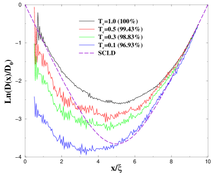
Figure 12: Local diffusion breaks down upon removing a small portion of high-transmission ($T>T_{c}$) states from the original ensemble. The source is placed at $x=0$. (from Ref. Tian10 with reproduction permission from C. S. Tian, S. K. Cheung, and Z. Q. Zhang $\copyright$ The American Physical Society)

VI.3 Roles of high transmission states

Dynamic studies of wave transport through localized samples Zhang09 have shown that the long-time transport in these systems is dominated by rare long-lived modes with high transmission coefficients (see Sec. II.2.1). This indicates that in the strongly localized regime far-reaching consequences may arise from the Lyapunov exponent fluctuations. To see this let us start from a semi-quantitative analysis. A basic prediction of the SCLD model Lagendijk00 is as follows that for localized samples $D(x)$ is a sum of two symmetric exponential decays truncated at the sample mid-point (see the dotted line in Fig. 4 which represents the left truncated exponential decay). This result may be written as

$$D(x)\sim\int_{0}^{\infty}d\gamma P(\gamma)e^{-\gamma{\rm min}(x,\,L-x)},\quad P(\gamma)=\delta(\gamma-\xi^{-1})$$ (141)

for $x$ sufficiently away from the interfaces, i.e., ${\rm min}(x,\,L-x)\gg\xi$. Importantly, the above distribution $P(\gamma)$ reflects the absence of fluctuations in the Lyapunov exponent. But this is correct only if the sample length is infinite. (That is, a semi-infinite sample is considered.) For finite-sized localized samples, the distribution $P(\gamma)$ is given by Eq. (8) instead. Replacing the Dirac distribution in Eq. (141) with the distribution (8) we reproduce the correct result for $D(x)$ namely Eq. (6), i.e.,

$$D(x) \sim \int_{0}^{\infty}d\gamma\,e^{-\frac{\xi L}{4}\left(\gamma-\xi^{-1}\right)^{2}}e^{-\gamma{\rm min}(x,\,L-x)}$$ (142)

$$\sim e^{-L/(4\xi)}\int_{0}^{\infty}d\gamma\,e^{-\frac{\xi L}{4}\gamma^{2}+\gamma|L/2-x|}\sim e^{-\frac{x(L-x)}{L\xi}}.$$

This clearly shows that the SCLD model completely ignores the fluctuations of the Lyapunov exponent. Interestingly, the second line in Eq. (142) shows that the integral is dominated by $\gamma\sim|1-2x/L|\xi^{-1}$. In particular, for $x$ closed to the sample center, the integral is dominated by the small $\gamma$ tail of the distribution $P(\gamma)$. This suggests that the significant enhancement of the local diffusion coefficient from the exponential decay near the sample center is deeply rooted in the rare high transmission states.

In Ref. Tian10 , the roles of high transmission states in the static transport are studied numerically, and data leading to results shown in Fig. 4 are further analyzed. First of all, $\ln T$ follows the normal distribution (8) Beenakker97 ; Anderson80 , with the average $\approx-L/\xi$ and variance $\approx 2L/\xi$. Then, to investigate the role of high transmission states a small portion of them (with transmission $T>T_{c}$) are removed from the original ensemble ($\omega=1.65c/a$ and $L/\xi=10$). Most of removed states are singly localized states, and the remainder (with a small portion) are necklace states Pendry94 . $D(x)/D_{0}$ is re-computed for the new ensemble. As shown in Fig. 12, even when the fraction of states removed is as small as $0.6\%$ (solid line, in red), the result deviates drastically from the original one (solid line, in black) and is asymmetric. This signals the breakdown of local diffusion and indicates that rare high-transmission states are intrinsic to local diffusion and novel scaling.

Substituting Eq. (6) into Eq. (131), we find

$$\langle T(L)\rangle\sim e^{-L/(4\xi)}.$$ (143)

We see that the dramatic enhancement of the resistivity near the sample center leads the system to exhibit a global localization behavior namely the exponential decay of the average transmission in the sample length, as we mentioned above. On the other hand, from the normal distribution of $P(\gamma)$ it follows that

$$\frac{d\langle\ln T(L)\rangle}{dL}=-\xi^{-1}.$$ (144)

Eqs. (143) and (144) show that (for both GOE and GUE systems,) the localization lengths obtained by the arithmetic and geometrical means of $T(L)$ differ by a factor of $4$. This factor arises from the rare disorder-induced resonant transmission, and previously was discovered for the conductance distribution Beenakker97 .

VII Conclusion

How do classical electromagnetic waves propagate through random open media? This is a long-standing fundamental issue in Anderson localization. One might expect that like many complex systems propagation of waves in random media bears the microscopic and macroscopic description simultaneously. The former is built upon the eigenmodes of the Maxwell equation which provide complete information on wave scattering (hence the term ‘microscopic’), while the latter describes the system in terms of a single macroscopic variable – the average energy density. It satisfies some macroscopic (generalized) diffusion equation which is valid only on the scale much larger than the mean free path (hence the term ‘macroscopic’). For open media, the microscopic description of waves can be traded to the superposition of excited quasi-normal modes. In contrast, the rational of the macroscopic description especially for strongly localized open media has been an open question explored by many researchers and had largely not been established as yet. This review is devoted to substantial recent progress achieved in the macroscopic (or ‘hydrodynamic’ called by condensed matter physicists) description of wave propagation in random open media.

We reviewed the recently developed first-principles theory for classical wave localization in open media Tian08 ; Tian10 that justifies unconventional macroscopic wave diffusion in these systems. In essence, it describes localization physics in terms of an effective action of the supermatrix $Q$ field. The theory differs crucially from the supersymmetric field theory of (electron) localization in infinite systems in the air-medium coupling action introduced by wave energy leakage through the interface. The latter breaks the translational symmetry of the low-energy field theory and constrains the supermatrix field by some boundary conditions. We showed at a pedagogical level how to use this theory to explicitly calculate the wave intensity profile and to establish a macroscopic description of wave propagation at a firm level.

We reviewed highly unconventional macroscopic wave diffusion in open media. This is described by a linear macroscopic equation – the local diffusion equation. It differs from the normal diffusion equation in that the diffusion coefficient is inhomogeneous in space. Most importantly, it was discovered in Ref. Tian10 that the local diffusion coefficient exhibits novel single parameter scaling. That is, it depends on the distance to the interface via a scaling factor proportional to the returning probability density, and the universal scaling function depends on both the system’s symmetry and dimensionality. In the static case (steady state), the scaling function in one dimensions has been found analytically giving the explicit analytic expression for the static local diffusion coefficient. These results are fully confirmed by numerical simulations. This suggests a profound new concept which is contrary to previous expectations. That is, the resonant transmission – formed in the scale of system’s size – does not wash out Fick’s law (thereby macroscopic diffusion) which is valid locally in space; rather, it results in novel scaling of the local diffusion coefficient which plays a decisive role in the long-time transport of localized waves.

From the practical view point, the novel scaling of the diffusion coefficient (127) and the local diffusion equation (4) are sufficient for theoretical analysis of many experimental measurements involving the averaged wave energy density. Such approach based on the macroscopic equation has the great advantage of technical simplicity over its sophisticated microscopic theory. In this case, one has to find the scaling function of the local diffusion coefficient by other methods (e.g., numerical simulations or fitting experimental data), and this is a relatively simple task.

We wish to mention some important directions in future studies. While the novel scaling of local diffusion coefficient has been shown to generally exist in the slab geometry in arbitrary dimensions, the non-perturbative scaling function remains to be worked out explicitly, and this could have far-reaching consequences. In fact, the dynamic local diffusion coefficient is related to a number of important issues. These include time-resolved transmissions Maret06 ; Zhang09 , the statistics of quasi-normal modes Genack11 , dynamic single parameter scaling Zhang09 , anomalously localized states and dynamic conductance Muzykantskii95 , etc.. Furthermore, the local diffusion coefficient (both dynamic and static) in high dimensions may help to reveal new physics due to the strong interplay between the openness of the medium and criticality. Indeed, we have seen that the novel scaling already leads to highly non-trivial results in one dimensions. That is, the localization length given by the mean transmission is four times larger than the typical localization length. We naturally expect that its effects in high dimensions might be even more interesting. Whether and to what extent the novel scaling of local diffusion coefficient affects the size-dependence of the conductance near Anderson transition? How does it lead to the pulsed wave decay on the output interface? These questions are fully open.

In this review, we have focused on ideal optical systems ignoring internal reflections at the boundary and absorption (gain) in the bulk. In experiments, these can have significant effects. Interestingly, there have been experimental and analytic evidence Tian12 showing that the common wisdom in optics – adding the extrapolation length to the sample length Niuwenhuizen – breaks down. The interplay between internal reflection and wave interference may lead to very rich localization behavior. The other issue, effects of (linear) absorption and gain in random media has received considerable attention John84 ; John85 ; Lai12 ; Kroha05 ; Kroha06 , but these works deal with infinite media. As far as realistic optical devices or experimental environments are concerned, one often deals with open media and this will lead to intriguing phenomena (for examples, see Refs. Genack06 ; Deysh05 ; Cao10 ; Zhang95 ; Beenakker96 ). A fundamental problem therefore is how these factors interact with localization and unconventional macroscopic diffusion.

The supersymmetric field theory reviewed here is formulated for scalar wave systems. As mentioned above, more complete studies of localization of classical electromagnetic waves will require a formulation for vector wave systems. What will be the symmetry of the supermatrix $Q$ and its low-energy action then? To what extent will the vector nature modify the macroscopics of localized waves in open media? These important questions are central to studies of light localization and largely unexplored. Throughout this review, we have focused on classical wave systems. In principle, the macroscopics reviewed here exists in electronic systems as well. As far as the latter is concerned, it is well known that the Anderson transition is classified into ten symmetry classes Altland96 . Of particular interests is the sympletic class. For this symmetry class, an intriguing phenomenon intrinsic to the openness of the system was discovered some time ago Zirnbauer92 . That is, even though an infinite Q$1$D disordered wire exhibits strong localization Efetov83a , the localization behavior is dramatically changed as long as the system is open (namely coupled to ideal leads): the conductance decreases to a constant instead of zero as the sample length goes to infinity. It is therefore conceivable that the symmetry may affect profoundly the behavior of the local diffusion coefficient.

Finally, we emphasize that throughout this review we consider only ensemble averaged observables. The theory reviewed here provides no information on individual disorder configurations. The resonant properties of individual disorder configurations in the localized regime can be studied by other approaches (see, e.g., Refs. Freilikher03 ; Freilikher04 ; Freilikher12 and references therein).

Appendix A The basics of Grassmann algebra and supermathematics

This Appendix includes some preliminary definitions and basic theorems of Grassmann algebra and supermathematics which are required for following (most) technical details of this review. We do not aim at a complete introduction to mathematical foundation of the supersymmetric field theory, for which we refer readers to Refs. Zirnbauer96 ; Efetov83 ; Efetov97 ; Berezin ; Berezin61 ; Berezin87 ; Zirnbauer85 ; Zirnbauer97 ; Zinn-Justin .

Grassmann algebra. The Grassmann algebra ${\cal A}$ (over complex $\mathbb{C}$) is an algebra constructed from $n$ generators $\chi_{i}$. These generators – the so-called Grassmannians – satisfy the anticommuting relation, i.e.,

$$\chi_{i}\chi_{j}+\chi_{j}\chi_{i}=0,\quad\forall{i,\,j}.$$ (145)

From this definition it follows that $\chi_{i}^{k}=0$ if the integer $k\geq 2$. This gives an important theorem: all elements in the Grassmann algebra ${\cal A}$ are first degree polynomials in each generator $\chi_{i}$. In other words, a generic function, $f(\chi_{1},\chi_{2},\cdots,\chi_{n})$, must be constructed from $2^{n}$ monomials, $\chi_{1}^{\alpha_{1}}\chi_{2}^{\alpha_{2}}\cdots\chi_{n}^{\alpha_{n}}$, where the power $\alpha_{k}$ takes the value of either $0$ or $1$, i.e.,

$$f(\chi_{1},\chi_{2},\cdots,\chi_{n})=\sum_{\{\alpha_{k}\}}c_{\alpha_{1}\alpha_{2}\cdots\alpha_{n}}\chi_{1}^{\alpha_{1}}\chi_{2}^{\alpha_{2}}\cdots\chi_{n}^{\alpha_{n}},$$ (146)

with the coefficient $c_{\alpha_{1}\alpha_{2}\cdots\alpha_{n}}\in\mathbb{C}$.

Define the reflection:

$$P(\chi_{i})=-\chi_{i}.$$ (147)

Then, a monomial of degree $k$ has a parity $(-1)^{k}$ for $P(\chi_{i_{1}}\chi_{i_{2}}\cdots\chi_{i_{k}})=(-1)^{k}\chi_{i_{1}}\chi_{i_{2}}\cdots\chi_{i_{k}}$. This divides the Grassmann algebra into two parts, ${\cal A}={\cal A}^{+}\cup{\cal A}^{-},\,{\cal A}^{+}\cap{\cal A}^{-}=\emptyset$, where ${\cal A}^{+}$ (${\cal A}^{-}$) has even (odd) parity, constructed from monomials of even (odd) number degree and therefore composed of commuting (anticommuting) elements. The former is a subalgebra in ${\cal A}$ whose elements are similar to ordinary complex numbers.

The complex conjugate operation (adjoint) of the Grassmann algebra is defined by

$$(\chi_{i})^{*}=\chi_{i}^{*},\quad(\chi_{i}^{*})^{*}=-\chi_{i},\quad(\chi_{i}\chi_{j})^{*}=\chi_{i}^{*}\chi_{j}^{*}.$$ (148)

The ‘$-$’ sign in the second relation makes $\chi_{i}^{*}\chi_{i}$ act like a ‘real number’, i.e., $(\chi_{i}^{*}\chi_{i})^{*}=\chi_{i}^{*}\chi_{i}$. Note that $\chi_{i}^{*}$ is independent of $\chi_{i}$ and as such, the complex conjugate of the Grassmann algebra is purely a formal definition.

Calculus in the Grassmann algebra. Eq. (146) allows us to introduce the partial derivative with respect to the generator $\chi_{i}$. Because any elements in the Grassmann algebra ${\cal A}$, which are functions of the generators, can be written as Eq. (146), we may move $\chi_{i}$ to the left for each term, obtaining

$$f=f_{0}+\chi_{i}f_{1},$$ (149)

where the coefficients $f_{0,1}$ are $\chi_{i}$-independent. Then, the left partial derivative with respect to $\chi_{i}$ is defined as

$$\frac{\partial f}{\partial\chi_{i}}\equiv f_{1}.$$ (150)

(The right partial derivative can be introduced in the similar way.) It is important that in moving $\chi_{i}$ to the left, a fermion sign is left due to the anticommuting relation (145). It is easy to check that the partial derivative defined by Eq. (150) is a nilpotent operator, i.e., $(\partial/\partial\chi_{i})^{2}=0$. Furthermore, if we consider $\chi_{i}$ as an operator acting on ${\cal A}$ via left-multiplication, then the nilpotent operator $\partial/\partial\chi_{i}$ and the operator $\chi_{i}$ constitute the Clifford algebra,

$$\chi_{i}\chi_{j}+\chi_{j}\chi_{i}=0,\quad\frac{\partial}{\partial\chi_{i}}\frac{\partial}{\partial\chi_{j}}+\frac{\partial}{\partial\chi_{j}}\frac{\partial}{\partial\chi_{i}}=0,\quad\chi_{i}\frac{\partial}{\partial\chi_{j}}+\frac{\partial}{\partial\chi_{j}}\chi_{i}=\delta_{ij}.$$ (151)

For Grassmann algebra, the integration operation is defined as the (left) derivative. More precisely, the single variable integration is defined as

$$\int fd\chi_{i}\equiv\frac{\partial}{\partial\chi_{i}}f,$$ (152)

while the multiple variable integration as

$$\int fd\chi_{k}\cdots d\chi_{1}\equiv\frac{\partial}{\partial\chi_{k}}\cdots\frac{\partial}{\partial\chi_{1}}f.$$ (153)

In fact, this formal definition satisfies the properties of the ordinary definite integral. To see this let us denote the integration defined in Eq. (152) as $I$. First of all, it is obviously a linear operator, $I[f_{1}+f_{2}]=I[f_{1}]+I[f_{2}]$ for $f_{1,2}\in{\cal A}$. Secondly, because the partial derivative is a nilpotent operator, we have $I[\partial f/\partial\chi_{i}]=0$ implying that the integral of a total derivative vanishes and $\partial I[f]/\partial\chi_{i}=0$ implying that a definite integral is a constant. Thirdly, if $f^{\prime}$ is $\chi_{i}$-independent, we have $I[ff^{\prime}]=I[f]f^{\prime}$: the overall factor can be pulled out of the integral (from the right). Finally, if we make the replacement $\chi_{i}\rightarrow\chi_{i}+\eta_{i}$, with $\eta_{i}$ a constant Grassmannian, the integral remains the same implying $d\chi_{i}=d(\chi_{i}+\eta_{i})$.

Gaussian integrals with Grassmannians. In this review we are interested in the case where the generator $\chi_{i}$ and its adjoint $\chi_{i}^{*}$ ($i=1,2,\cdots,n$) appear in pairs. Consider an invertible $n\times n$ matrix, $M$, with the entries $M_{ij}\in\mathbb{C}$. By Taylor expanding $e^{-\chi^{*}_{i}M_{ij}\chi_{j}}$ and using Eq. (153), one finds an important identity,

$$\int e^{-\chi^{*}_{i}M_{ij}\chi_{j}}d\chi^{*}_{1}d\chi_{1}\cdots d\chi^{*}_{n}d\chi_{n}={\rm det}M.$$ (154)

This is in sharp contrast to the Gaussian integral over ordinary complex variables, $S_{i}^{*},S_{i},i=1,2,\cdots,n$, which is

$$\int e^{-S^{*}_{i}M_{ij}S_{j}}\frac{dS^{*}_{1}dS_{1}}{\pi}\cdots\frac{dS^{*}_{n}dS_{n}}{\pi}=({\rm det}M)^{-1}.$$ (155)

Importantly, the difference of the power of the determinant, $\pm 1$, on the right-hand side of Eqs. (154) and (155) reflect different rules of the change of variables for Grassmiannians and complex variables. Indeed, the linear transformations: $\chi^{\prime}\equiv M\chi$ and $S^{\prime}\equiv MS$ lead to $d\chi_{n}\cdots d\chi_{1}=\det M\,d\chi^{\prime}_{n}\cdots d\chi^{\prime}_{1}$ while $dS_{n}\cdots dS_{1}=(\det M)^{-1}\,dS^{\prime}_{n}\cdots dS^{\prime}_{1}$. By using Eq. (154), we obtain another important identity:

$$({\rm det}M)^{-1}\int\chi_{i}\chi^{*}_{j}e^{-\chi_{i}^{*}M_{ij}\chi_{j}}d\chi^{*}_{1}d\chi_{1}\cdots d\chi^{*}_{n}d\chi_{n}=(M^{-1})_{ij}.$$ (156)

The supervector and the supermatrix. A supervector $\phi$ is composed of an $n$-anticommuting component vector $\chi$ and an $m$-commuting component vector $S$, (We shall consider the case of $n=m$.)

$$\phi\equiv\left(\begin{array}[]{c}\chi\\ S\\ \end{array}\right),\quad\chi=\left(\begin{array}[]{c}\chi_{1}\\ \vdots\\ \chi_{n}\\ \end{array}\right),\quad S=\left(\begin{array}[]{c}S_{1}\\ \vdots\\ S_{n}\\ \end{array}\right),$$ (165)

where $\chi_{i}$ ($S_{i}$) are anticommuting (commuting) variables. All such supervectors constitute a linear space, $\Phi_{n,n}$. The transpose of the supervector $\phi$ is defined by

$$\phi^{\rm T}\equiv(\chi_{1}\cdots\chi_{n}S_{1}\cdots S_{n}),$$ (166)

while its Hermitian conjugate by

$$\phi^{\dagger}\equiv(\chi^{*}_{1}\cdots\chi^{*}_{n}S^{*}_{1}\cdots S^{*}_{n}).$$ (167)

The inner product on the supervector space $\Phi_{n,n}$ is defined by

$$(\phi,\phi^{\prime})\equiv\phi^{\dagger}\phi^{\prime}=\sum_{i=1}^{n}\chi^{*}_{i}\chi^{\prime}_{i}+\sum_{i=1}^{n}S^{*}_{i}S^{\prime}_{i},\quad\forall\phi,\,\phi^{\prime}\in\Phi_{n,n}.$$ (168)

The norm $\sqrt{(\phi,\phi)}$ defines the ‘length’ of a supervector $\phi$.

The linear transformation on the supervector space $\Phi_{n,n}$ is described by a supermatrix, $M$, which transfers anticommuting (fermionic) into commuting (bosonic) components and vice versa. It has the following structure,

$$M\equiv\left(\begin{array}[]{cc}M_{\rm FF}&M_{\rm FB}\\ M_{\rm BF}&M_{\rm BB}\\ \end{array}\right)^{\rm fb},$$ (171)

with the superscript ‘fb’ standing for the fermion-boson space accounting for the supervector structure defined in the first relation of Eq. (165). Here, $M_{\rm FF}$, $M_{\rm BB}$, $M_{\rm FB}$, and $M_{\rm BF}$ are $n\times n$ matrices. Furthermore, the entries of diagonal (off-diagonal) blocks, $M_{\rm BB},\,M_{\rm FF}$ ($M_{\rm BF},\,M_{\rm FB}$), are commuting (anticommuting) variables belonging to ${\cal A}^{+}$ (${\cal A}^{-}$). The supermatrix product is defined as usual.

The transpose of the supermatrix is defined by $({\rm M\phi})^{\rm T}\phi^{\prime}\equiv\phi^{\rm T}M^{\rm T}\phi^{\prime},\,\forall\phi,\,\phi^{\prime}\in\Phi_{n,n}$. This gives

$$M^{\rm T}=\left(\begin{array}[]{cc}M_{\rm FF}^{\rm T}&-M_{\rm BF}^{\rm T}\\ M_{\rm FB}^{\rm T}&M_{\rm BB}^{\rm T}\\ \end{array}\right)^{\rm fb},$$ (174)

where the ‘$-$’ sign in the upper right block arises from the anticommuting relation, and for each block $M_{\alpha\alpha^{\prime}}$ the transpose is defined as usual. By the definition one may easily check that for two supermatrices, $M,\,M^{\prime}$,

$$(MM^{\prime})^{\rm T}=M^{\prime\rm T}M^{\rm T},$$ (175)

$$(M\phi)^{\rm T}=\phi^{\rm T}M^{\rm T}.$$ (176)

The Hermitian conjugate of the supermatrix is defined by $({\rm M\phi},\phi^{\prime})\equiv(\phi,M^{\dagger}\phi^{\prime}),\,\forall\phi,\,\phi^{\prime}\in\Phi_{n,n}$. This gives $M^{\dagger}=(M^{\rm T})^{*}$. The pseudounitary transformation can be defined as such $U$ that conserves the metric tensor $K$, i.e., $(U\phi,KU\phi^{\prime})\equiv(\phi,K\phi^{\prime})$ or $U^{\dagger}KU=K$. If $K=\mathbbm{1}$, then $U$ becomes unitary. Using the identity (175) and the third relation in Eq. (148), we have

$$(MM^{\prime})^{\dagger}=M^{\prime\dagger}M^{\dagger}.$$ (177)

By using Eq. (174) and the second relation in Eq. (148), we have

$$(M^{\dagger})^{\dagger}=M,$$ (178)

which should be contrasted with $(M^{\rm T})^{\rm T}=\sigma_{3}^{\rm fb}M\sigma_{3}^{\rm fb}$.

For the supermatrix, we introduce the supertrace, denoted as ‘str’,

$${\rm str}M\equiv{\rm tr}M_{\rm FF}-{\rm tr}M_{\rm BB},$$ (179)

where ‘tr’ stands for the normal trace. (This differs from that defined in some other references, e.g., Refs. Zirnbauer84 ; Zirnbauer05 , by a minus sign.) By using the definition, it is easy to check the following relations,

$${\rm str}(MM^{\prime})={\rm str}(M^{\prime}M)$$ (180)

and

$$(\phi,M\phi^{\prime})=-{\rm str}(M\phi^{\prime}\otimes\phi^{\dagger}).$$ (181)

The superdeterminant is defined by

$$\ln{\rm sdet}M\equiv{\rm str}\ln M,$$ (182)

which is the direct generalization of the well-known identity $\ln\det(\cdot)={\rm tr}\ln(\cdot)$. This gives

$${\rm sdet}M\equiv{\rm det}(M_{\rm FF}-M_{\rm FB}M_{\rm BB}^{-1}M_{\rm BF})({\rm det}M_{\rm BB})^{-1}.$$ (183)

By the definition we have

$${\rm sdet}(MM^{\prime})={\rm sdet}\,M{\rm sdet}M^{\prime}.$$ (184)

By using Eqs. (174) and (183), we can show

$${\rm sdet}\,M^{\rm T}={\rm sdet}\,M.$$ (185)

Gaussian integrals with supervectors. Given the supermatrix $M$, we have the following Gaussian integral over the supervector,

$$\int e^{-\phi^{\dagger}M\phi}d\phi^{\dagger}d\phi={\rm sdet}M,$$ (186)

where the measure $d\phi^{\dagger}d\phi\equiv\prod_{i=1}^{n}d\chi_{i}^{*}d\chi_{i}\prod_{i=1}^{m}\frac{dS_{i}^{*}dS_{i}}{\pi}$, and

$$({\rm sdet}M)^{-1}\int\phi_{i}\phi^{*}_{j}e^{-\phi^{\dagger}M\phi}d\phi^{\dagger}d\phi=(M^{-1})_{ij}.$$ (187)

In Eq. (187), if the pre-exponential factor is a product of $\phi$’s with the number $>2$, then the ordinary Wick theorem holds. The only difference is that exchanging Grassmannians leads to a fermionic sign. It is very important that here, we have assumed the convergence of the integral, i.e., ${\rm Re}\,S^{\dagger}M_{\rm BB}S>0$.

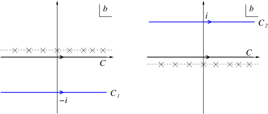
Figure 13: Contour deformation for the integral over the matrix element $b_{1t,1t}$ (left) and $b_{2t,2t}$ (right).

Appendix B The diagonal mean-field saddle points

In this Appendix we will find the diagonal solutions to the saddle point equation (55), i.e., $Q_{0}={\rm diag}\,\{q_{i}\}$. (Recall that the index $i=m\alpha t$.) Substituting $Q_{0}$ into Eq. (55) gives

$$q_{i} = \frac{1}{2}i\omega^{2}\Delta\int\frac{d{\bf k}}{(2\pi)^{d}}\frac{1}{{\bf k}^{2}-\omega^{2}+2i\omega^{2}q_{i}}=\frac{1}{2}i\omega^{2}\Delta\int_{0}^{\infty}dk\nu(k)\frac{1}{k^{2}-\omega^{2}+2i\omega^{2}q_{i}}$$ (188)

$$= \frac{1}{4}i\omega^{2}\Delta\int_{-\infty}^{\infty}dk\nu(|k|)\frac{1}{k^{2}-\omega^{2}+2i\omega^{2}q_{i}}.$$

Notice that depending on the dimension this integral may suffer ultraviolet divergence. In this case, since the wavelength of photons has no lower bound, one may cure this divergence by multiplying the integrand by a factor $e^{\pm i\delta\zeta}$, where the ‘$+$’(‘$-$’) sign corresponds to ${\rm Re}q_{i}<0\,(>0)$, and send the positive infinitesimal $\delta$ to zero in the end. (A more physical way of curing this divergence is to introduce more realistic disorders as discussed in Sec. IV.1.4. In any case, this divergence only enters into the renormalization of the background value of the refractive index which is unimportant for present discussions.) In the limit $\Delta\omega\nu(\omega)\ll 1$ this transcendental equation is solvable, giving

$$q_{i}=\pm|{\rm Re}\,q_{i}|+i{\rm Im}\,q_{i},\quad|{\rm Re}\,q_{i}|=\frac{\pi}{4}\Delta\omega\nu(\omega)+o(\Delta\omega\nu(\omega)),\,{\rm Im}\,q_{i}=o(\Delta\omega\nu(\omega)).$$ (189)

That is,

$$q_{i}=\frac{\pi}{4}\Delta\omega\nu(\omega)\lambda_{i}=\tilde{q}\lambda_{i},\quad\lambda_{i}=\pm 1.$$ (190)

At the first glance, Eq. (190) gives $2^{8}=256$ solutions. But this is not true. First of all, due to the charge conjugation symmetry, $Q=CKQ^{\rm T}KC^{\rm T}$ that inherits from the reality condition (38),

$$\lambda_{m\alpha 1}=\lambda_{m\alpha 2}.$$ (191)

Secondly, for the functional integral (53) to converge, it is necessary that $Q_{m{\rm B}t,m{\rm B}t}$ is purely imaginary. Therefore, the saddle points (190) do not belong to this manifold. To solve this problem, in integrating out the matrix elements $Q_{m{\rm B}t,m{\rm B}t}$, we deform the integral contour such that (i) no singularities of the action $F[Q]$ are encountered, and (ii) the new contour passes $q_{1{\rm B}t}=+\tilde{q}$ ($\lambda_{1{\rm B}t}=+1$) and $q_{2{\rm B}t}=-\tilde{q}$ ($\lambda_{2{\rm B}t}=-1$), where the ‘$+$’ (‘$-$’) sign accounts for the analytic structure of the advanced (retarded) Green function. To ensure the condition (i) we should first look for the singularities of the integrand of the partition function (53). According to the definitions (182) and (183), they are the zeros of ${\rm det}(-\nabla^{2}-\omega^{2}+\omega\tilde{\omega}^{+}\sigma_{3}^{\rm ar}\otimes{\mathbbm{1}}^{\rm tr}+2i\omega^{2}Q_{\rm BB})$. Defining $Q_{\rm BB}=ib$, we find that for the integral over the diagonal entries, $b_{1t,1t}\in\mathbb{R}$, the singularities lie at the line ${\rm Im}b_{1t,1t}=\delta>0$. (Recall that $\tilde{\omega}^{+}=\tilde{\omega}+i\delta$.) Taking this into account, we deform the contour, $C$, into $C_{1}$ that passes through $b_{1t,1t}=-i\tilde{q}$, corresponding to $\lambda_{1{\rm B}t}=1$ (Fig. 13, left). Similarly, for the integral over the diagonal entries, $b_{2t,2t}$, the singularities lie at the line ${\rm Im}b_{2t,2t}=\delta<0$. Therefore, we deform the contour into $C_{2}$ that passes through $b_{2t,2t}=i\tilde{q}$, corresponding to $\lambda_{2{\rm B}t}=-1$ (Fig. 13, right). For the other cases, i.e., $\lambda_{1{\rm B}t}=-1$ and (or) $\lambda_{2{\rm B}t}=1$, to perform the corresponding contour deformation must cross the singularities. Such saddle points are unphysical and must be discarded. Thus, we have

$$\lambda_{1{\rm B}t}=-\lambda_{2{\rm B}t}=1.$$ (192)

Taking Eqs. (191) and (192) into account, now we have only four possibilities namely $\lambda_{1{\rm F}1}=\lambda_{1{\rm F}2}=\pm 1$ and $\lambda_{2{\rm F}1}=\lambda_{2{\rm F}2}=\pm 1$. Integrating out fluctuations around the saddle points with $\lambda_{1{\rm F}t}=\lambda_{2{\rm F}t}$ leads to a negligible small factor because the bosonic and fermionic degrees of freedom do not compensate. Therefore, the two saddle points of $\lambda_{1{\rm F}t}=\lambda_{2{\rm F}t}$ do not play any roles. Finally, only two saddle points out of $256$ possibilities are left: $\Lambda$ and $-k\Lambda$. Andreev and Altshuler discovered Altshuler95 ; Altshuler96 that both are the stationary points of the action (69). The former (latter) determines the perturbative (non-perturbative) part of the level correlator in finite closed systems.

Appendix C Derivation of the fluctuation action

The neighborhood of $Q_{0}=T_{0}^{-1}(\tilde{q}\Lambda)T_{0}$ in the supermatrix space can be parametrized by $Q_{0}+\delta Q=(T_{0}(1+\delta T))^{-1}(\tilde{q}\Lambda+\delta\Lambda)(T_{0}(1+\delta T))$. Here $\delta T$ and $\delta\Lambda$ parametrize fluctuations in the coset space and eigenvalues, respectively. Expanding $\delta T$ and $\delta\Lambda$, we obtain the fluctuation $\delta Q\approx T_{0}^{-1}\delta\Lambda T_{0}+[Q_{0},\delta T]$. It is easy to see that the first (second) term (anti)commutes with $Q_{0}$. Therefore, the former (latter) may be identified as $\delta Q^{l}$ ($\delta Q^{t}$). In other words, the eigenvalue fluctuations generate the longitudinal components while the fluctuations in the coset space generate the transverse components. The former violates the nonlinear constraint (i.e., $Q^{2}$ is a constant matrix) and thereby brings $Q_{0}$ out of the saddle point manifold.

In the remainder of this Appendix we derive the fluctuation (63). Upon the substitution of the decomposition $\delta Q_{\bf q}=\delta Q_{\bf q}^{l}+\delta Q_{\bf q}^{t}$, we simplify Eq. (62) to

$$\int\frac{d{\bf q}}{(2\pi)^{d}}{\rm str}\left({\cal H}_{\bf q}^{l}\delta Q_{\bf q}^{l}\delta Q_{-{\bf q}}^{l}+{\cal H}_{\bf q}^{t}\delta Q_{\bf q}^{t}\delta Q_{-{\bf q}}^{t}\right),$$ (193)

$${\cal H}_{\bf q}^{l}\equiv\Delta^{-1}+\omega^{4}\int\frac{d{\bf k}}{(2\pi)^{d}}{\cal G}_{0}\left({\bf k}+\frac{{\bf q}}{2},Q_{0}\right){\cal G}_{0}\left({\bf k}-\frac{{\bf q}}{2},Q_{0}\right),$$

$${\cal H}_{\bf q}^{t}\equiv\Delta^{-1}+\omega^{4}\int\frac{d{\bf k}}{(2\pi)^{d}}{\cal G}_{0}\left({\bf k}+\frac{{\bf q}}{2},Q_{0}\right){\cal G}_{0}\left({\bf k}-\frac{{\bf q}}{2},-Q_{0}\right).$$

To simplify the action of the longitudinal components, we notice

$$\int\frac{d{\bf k}}{(2\pi)^{d}}{\cal G}_{0}\left({\bf k}+\frac{{\bf q}}{2},Q_{0}\right){\cal G}_{0}\left({\bf k}-\frac{{\bf q}}{2},Q_{0}\right)=\int\frac{d{\bf k}}{(2\pi)^{d}}{\cal G}_{0}\left({\bf k}+\frac{{\bf q}}{2},T_{0}^{-1}(\tilde{q}\Lambda)T_{0}\right){\cal G}_{0}\left({\bf k}-\frac{{\bf q}}{2},T_{0}^{-1}(\tilde{q}\Lambda)T_{0}\right)$$ (194)

$$= T_{0}^{-1}\left[\int\frac{d{\bf k}}{(2\pi)^{d}}{\cal G}_{0}\left({\bf k}+\frac{{\bf q}}{2},\tilde{q}\Lambda\right){\cal G}_{0}\left({\bf k}-\frac{{\bf q}}{2},\tilde{q}\Lambda\right)\right]T_{0}$$

$$= T_{0}^{-1}{\rm diag}\left\{\int\frac{d{\bf k}}{(2\pi)^{d}}{\cal G}_{0}\left({\bf k}+\frac{{\bf q}}{2},\tilde{q}\lambda_{i}\right){\cal G}_{0}\left({\bf k}-\frac{{\bf q}}{2},\tilde{q}\lambda_{i}\right)\right\}T_{0},$$

where in deriving the last line, we have used the fact that $\Lambda={\rm diag}\,\{\lambda_{i}\}$ with $\lambda_{1\alpha t}=-\lambda_{2\alpha t}=1$. Because

$$\int\frac{d{\bf k}}{(2\pi)^{d}}{\cal G}_{0}\left({\bf k}+\frac{{\bf q}}{2},\tilde{q}\lambda_{i}\right){\cal G}_{0}\left({\bf k}-\frac{{\bf q}}{2},\tilde{q}\lambda_{i}\right)\approx\int\frac{d{\bf k}}{(2\pi)^{d}}{\cal G}_{0}\left({\bf k},\tilde{q}\lambda_{i}\right){\cal G}_{0}\left({\bf k},\tilde{q}\lambda_{i}\right)$$ (195)

$$= \frac{1}{2}\int_{-\infty}^{\infty}dk\nu(|k|)\frac{1}{(k^{2}-\omega^{2}+2i\omega^{2}\tilde{q}\lambda_{i})^{2}}=0,$$

we have ${\cal H}_{\bf q}^{l}=\Delta^{-1}$. Here, the same ultraviolet regularization as Eq. (188) was used.

To simplify the action of the transverse components, we notice

$$\int\frac{d{\bf k}}{(2\pi)^{d}}{\cal G}_{0}\left({\bf k}+\frac{{\bf q}}{2},Q_{0}\right){\cal G}_{0}\left({\bf k}-\frac{{\bf q}}{2},-Q_{0}\right)$$ (196)

$$= T_{0}^{-1}{\rm diag}\left\{\int\frac{d{\bf k}}{(2\pi)^{d}}{\cal G}_{0}\left({\bf k}+\frac{{\bf q}}{2},\tilde{q}\lambda_{i}\right){\cal G}_{0}\left({\bf k}-\frac{{\bf q}}{2},-\tilde{q}\lambda_{i}\right)\right\}T_{0}$$

$$= -T_{0}^{-1}{\rm diag}\left\{\int\frac{d{\bf k}}{(2\pi)^{d}}\frac{1}{[({\bf k}+{\bf q}/2)^{2}-\omega^{2}+2i\omega^{2}\tilde{q}\lambda_{i}][({\bf k}-{\bf q}/2)^{2}-\omega^{2}-2i\omega^{2}\tilde{q}\lambda_{i}]}\right\}T_{0}.$$

Since the integral over ${\bf k}$ is dominated by the shell of $|{\bf k}|\approx\omega$, we have $|{\bf k}\cdot{\bf q}|\gg|{\bf q}|^{2}$. As a result, ${\cal H}_{\bf q}^{t}$ is simplified to

$${\cal H}_{\bf q}^{t} = \Delta^{-1}-\omega^{4}T_{0}^{-1}{\rm diag}\left\{\int\frac{d{\bf k}}{(2\pi)^{d}}\frac{1}{[{\bf k}^{2}+{\bf k}\cdot{\bf q}-\omega^{2}+2i\omega^{2}\tilde{q}\lambda_{i}][{\bf k}^{2}-{\bf k}\cdot{\bf q}-\omega^{2}-2i\omega^{2}\tilde{q}\lambda_{i}]}\right\}T_{0}$$ (197)

$$\approx \Delta^{-1}-\Delta^{-1}T_{0}^{-1}{\rm diag}\left\{\int\frac{d\Omega_{d}}{\Omega_{d}}\frac{1}{1-i\frac{2}{\pi\Delta\omega^{2}\nu(\omega)}{\hat{n}}\cdot{\bf q}}\right\}T_{0}$$

$$= \Delta^{-1}\left\{1-\int\frac{d\Omega_{d}}{\Omega_{d}}\frac{1}{1-i\frac{2}{\pi\Delta\omega^{2}\nu(\omega)}{\hat{n}}\cdot{\bf q}}\right\}$$

$$\approx \Delta^{-1}\left\{1-\left[1-\frac{1}{d}\left(\frac{2}{\pi\Delta\omega^{2}\nu(\omega)}\right)^{2}{\bf q}^{2}\right]\right\}=\frac{1}{d\Delta}\left(\frac{2}{\pi\Delta\omega^{2}\nu(\omega)}\right)^{2}{\bf q}^{2},$$

where ${\hat{n}}$ is the unit vector in the $d$-dimensional unit sphere of volume $\Omega_{d}$.

Substituting Eq. (197) into Eq. (C) gives

$$\Delta^{-1}\left(\int\frac{d{\bf q}}{(2\pi)^{d}}{\rm str}\{\delta Q_{\bf q}^{l}\delta Q_{-{\bf q}}^{l}\}+\frac{1}{d}\left(\frac{2}{\pi\Delta\omega^{2}\nu(\omega)}\right)^{2}\int\frac{d{\bf q}}{(2\pi)^{d}}|{\bf q}|^{2}{\rm str}\{{\delta Q}^{t}_{{\bf q}}{\delta Q}^{t}_{-{\bf q}}\}\right).$$ (198)

Upon inserting this action into the partition function (53), we may integrate out the longitudinal components, $\delta Q_{{\bf q}}^{l}$. Such a Gaussian integral is unity because the degrees of freedom of commuting and anticommuting variables compensate each other. The remaining action is a functional of the transverse components only which is

$$\frac{1}{d\Delta}\left(\frac{2}{\pi\Delta\omega^{2}\nu(\omega)}\right)^{2}\int d{\bf r}{\rm str}(\nabla{\delta Q}^{t}({\bf r}))^{2}.$$ (199)

Since $(Q_{0}+\delta Q^{t}({\bf r}))$ stays inside the manifold defined by Eq. (57), we have $\nabla{\delta Q}^{t}({\bf r})=\tilde{q}\nabla(T^{-1}({\bf r})\Lambda T({\bf r}))$. Eq. (199) then gives the fluctuation action (63).

Appendix D Derivation of the interface action

In this Appendix, we will derive the interface action $F_{\rm int}[Q]$ with the help of the Zirnbauer-Efetov theorem. Formally, Eq. (81) differs from Eq. (15) only in the non-Hermitian part of the effective Hamiltonian, i.e., $\pm i{\hat{B}}\delta_{C}$. Therefore, we may repeat the procedures of Sec. IV.1.2. As a result,

$$F_{\rm int}[Q]=-\frac{1}{2}\,{\rm str}_{{\bf r}}\ln\,\left(1-{\hat{B}}\Lambda{\cal G}_{0}\right),$$ (200)

where the supertrace ‘${\rm str}_{{\bf r}}$’ includes the integral over the spatial coordinates. Near the interface we may choose locally the coordinate system as ${\bf r}\equiv({\bf r}_{\perp},z)$ where the first $(d-1)$ coordinates give the projection to the interface $C$ and the last one the distance to the interface. Note that the $z$-axis points towards the random medium. As shown in Sec. IV.1.3, (inside the random medium) the matrix Green function ${\cal G}_{0}$ exponentially decays in space with a characteristic length of the order of the mean free path. Moreover, both $Q$ and the dielectric field vary over a scale much larger than the mean free path. Taking these into account, we find

$${\cal G}_{0}({\bf r},{\bf r}^{\prime};Q({\bf r}^{\prime}))\approx\frac{2}{\pi i}\int\frac{d^{d-1}{\bf k}_{\perp}}{(2\pi)^{d-1}}\int_{0}^{\infty}dk\frac{e^{i{\bf k}_{\perp}\cdot({\bf r}_{\perp}-{\bf r}^{\prime}_{\perp})}\cos(kz)\cos(kz^{\prime})}{(\omega({\bf r}^{\prime}))^{2}-|{\bf k}_{\perp}|^{2}-k^{2}+i\frac{\omega({\bf r}^{\prime})}{l({\bf r}^{\prime})}Q({\bf r}^{\prime})},\quad{\bf r},{\bf r}^{\prime}\in{\cal V}_{+}.$$ (201)

Here, $(\omega({\bf r}))^{2}=\omega^{2}(1+\overline{\epsilon({\bf r})})$, with $(1+\overline{\epsilon({\bf r})})$ the local average refractive index near the interface which generally causes the internal reflection. Because $\omega({\bf r})$ locally depends on the average refractive index, from Eq. (64) we find that near the interface the mean free path $l$ generally acquires a ${\bf r}$-dependence also.

On the other hand, the Green function $g^{R}_{\omega^{2}}({\bf r},{\bf r}^{\prime})$ is

$$g_{\omega^{2}}^{R}({\bf r},{\bf r}^{\prime})=\frac{2}{\pi}\int\frac{d^{d-1}{\bf k}_{\perp}}{(2\pi)^{d-1}}\int_{0}^{\infty}dk\frac{e^{i{\bf k}_{\perp}\cdot({\bf r}_{\perp}-{\bf r}_{\perp}^{\prime})}\,\sin(kz)\sin(kz^{\prime})}{\omega^{2}-{\bf k}_{\perp}^{2}-k^{2}+i0^{+}},\quad{\bf r},{\bf r}^{\prime}\in{\cal V}_{-}.$$ (202)

Substituting it into Eq. (82) gives

$$({\hat{B}}f)\,({\bf r}_{\perp})=\int\frac{d^{d-1}{\bf k}_{\perp}}{(2\pi)^{d-1}}\int d^{d-1}{\bf r}_{\perp}^{\prime}\,\sqrt{\omega^{2}-|{\bf k}_{\perp}|^{2}}\,e^{i{\bf k}_{\perp}\cdot({\bf r}_{\perp}-{\bf r}_{\perp}^{\prime})}\,f({\bf r}_{\perp}^{\prime})\,.$$ (203)

Let us insert Eqs. (201) and (203) into Eq. (200). As a result,

$$F_{\rm int}[Q]=-\frac{1}{2}\int d{\bf r}_{\perp}\int_{|{\bf k}_{\perp}|\leq\omega}\frac{d^{d-1}{\bf k}_{\perp}}{(2\pi)^{d-1}}\,{\rm str}\ln\left(1+\alpha_{{\bf k}_{\perp}}({\bf r})\,\Lambda Q({\bf r})\right),$$ (204)

where the coefficient

$$\alpha_{{\bf k}_{\perp}}({\bf r})=\sqrt{\frac{\omega^{2}-|{\bf k}_{\perp}|^{2}}{\omega^{2}\left(1+\overline{\epsilon({\bf r})}\right)-|{\bf k}_{\perp}|^{2}}}.$$ (205)

In deriving Eq. (204) we have adopted the trick used in Appendix C. That is, we made the local gauge transformation so that $Q({\bf r})$ becomes diagonal, and after integrating out $k$ we rotated the diagonal matrix back to $Q({\bf r})$. Eq. (204) can be rewritten as Eq. (83) Tian08 , where the internal reflection coefficient is

$$R_{{\bf k}_{\perp}}({\bf r})=\left|\frac{1-\alpha_{{\bf k}_{\perp}}({\bf r})}{1+\alpha_{{\bf k}_{\perp}}({\bf r})}\right|^{2},$$ (206)

in agreement with the well-known result Landau .

Appendix E Derivation of Eq. (110)

First of all, we have

$$F_{2}[W] = \frac{\pi\nu}{2}\int d{\bf r}{\rm str}\left(-2D_{0}(\nabla iW)^{2}(iW)^{2}+i\tilde{\omega}(iW)^{4}\right)$$ (207)

$$= \frac{\pi\nu}{2}\int d{\bf r}{\rm str}\left(2D_{0}\left(\nabla^{2}iW(iW)^{3}+\left(\nabla iWiW\right)^{2}+\left(\nabla iW\right)^{2}(iW)^{2}\right)+i\tilde{\omega}(iW)^{4}\right),$$

where in deriving the second line we have used the integral by parts. Let us substitute it into the expansion (106). This leads to the leading wave interference correction to the bare correlator $\delta{\cal Y}_{1}({\bf r},{\bf r}^{\prime};\tilde{\omega})$. The latter has five nonvanishing contributions, i.e., $\delta{\cal Y}_{1}({\bf r},{\bf r}^{\prime};\tilde{\omega})=\delta{\cal Y}_{1a}+\delta{\cal Y}_{1b}+\delta{\cal Y}_{1c}+\delta{\cal Y}_{1d}+\delta{\cal Y}_{1e}$. The first term is

$$\delta{\cal Y}_{1a}\equiv-\left(\frac{\pi\nu(\omega)}{4\omega}\right)^{2}\left\langle{\rm str}A_{+}iW({\bf r})A_{-}(iW({\bf r}^{\prime}))^{3}+{\rm str}A_{+}(iW({\bf r}))^{3}A_{-}iW({\bf r}^{\prime})\right\rangle_{0}$$ (208)

corresponding to the diagram given in Fig. 8 (b). The other terms are

$$\delta{\cal Y}_{1b} \equiv \left(\frac{\pi\nu(\omega)}{4\omega}\right)^{2}\pi\nu D_{0}\int d{\bf r}_{1}\left\langle{\rm str}A_{+}iW({\bf r})A_{-}iW({\bf r}^{\prime}){\rm str}\nabla^{2}iW({\bf r}_{1})(iW({\bf r}_{1}))^{3}\right\rangle_{0},$$

$$\delta{\cal Y}_{1c} \equiv \left(\frac{\pi\nu(\omega)}{4\omega}\right)^{2}\frac{i\pi\nu\tilde{\omega}}{2}\int d{\bf r}_{1}\left\langle{\rm str}A_{+}iW({\bf r})A_{-}iW({\bf r}^{\prime}){\rm str}(iW({\bf r}_{1}))^{4}\right\rangle_{0},$$

$$\delta{\cal Y}_{1d} \equiv \left(\frac{\pi\nu(\omega)}{4\omega}\right)^{2}\pi\nu D_{0}\int d{\bf r}_{1}\left\langle{\rm str}A_{+}iW({\bf r})A_{-}iW({\bf r}^{\prime}){\rm str}(\nabla iW({\bf r}_{1})iW({\bf r}_{1}))^{2}\right\rangle_{0},$$

$$\delta{\cal Y}_{1e} \equiv \left(\frac{\pi\nu(\omega)}{4\omega}\right)^{2}\pi\nu D_{0}\int d{\bf r}_{1}\left\langle{\rm str}A_{+}iW({\bf r})A_{-}iW({\bf r}^{\prime}){\rm str}(\nabla iW({\bf r}_{1}))^{2}(iW({\bf r}_{1}))^{2}\right\rangle_{0}$$ (209)

given by Fig. 8 (a).

For $\delta{\cal Y}_{1b}$ let us now make the first contraction by using the rules (V.1.2) and start from the $W$-factor acted by the operator $\nabla^{2}$. There are three possibilities, leading to

$$\delta{\cal Y}_{1b} = \left(\frac{\pi\nu(\omega)}{4\omega}\right)^{2}\pi\nu D_{0}\int d{\bf r}_{1}\Bigg{\{}\left\langle{\rm str}A_{+}iW({\bf r})A_{-}\mathord{\leavevmode\hbox to14.28pt{\vbox to13.5pt{\text{[drawing]}}}}({\bf r}^{\prime}){\rm str}\nabla^{2}\mathord{\leavevmode\hbox to14.28pt{\vbox to13.5pt{\text{[drawing]}}}}({\bf r}_{1})(iW({\bf r}_{1}))^{3}\leavevmode\hbox to0.4pt{\vbox to4.83pt{\text{[drawing]}}}\right\rangle_{0} iW iW$$ (210)

$$+\left\langle{\rm str}A_{+}\mathord{\leavevmode\hbox to14.28pt{\vbox to13.5pt{\text{[drawing]}}}}({\bf r})A_{-}iW({\bf r}^{\prime}){\rm str}\nabla^{2}\mathord{\leavevmode\hbox to14.28pt{\vbox to13.5pt{\text{[drawing]}}}}({\bf r}_{1})(iW({\bf r}_{1}))^{3}\leavevmode\hbox to0.4pt{\vbox to4.83pt{\text{[drawing]}}}\right\rangle_{0} iW iW iW iW$$

$$+\left\langle{\rm str}A_{+}iW({\bf r})A_{-}iW({\bf r}^{\prime}){\rm str}\nabla^{2}\mathord{\leavevmode\hbox to14.28pt{\vbox to13.5pt{\text{[drawing]}}}}({\bf r}_{1})iW({\bf r}_{1})\mathord{\leavevmode\hbox to14.28pt{\vbox to13.5pt{\text{[drawing]}}}}({\bf r}_{1})iW({\bf r}_{1})\leavevmode\hbox to0.4pt{\vbox to4.83pt{\text{[drawing]}}}\right\rangle_{0}\Bigg{\}}=\delta{\cal Y}^{\prime}_{1b}+\delta{\cal Y}^{\prime\prime}_{1b}, iW iW$$

where

$$\delta{\cal Y}^{\prime}_{1b} = \left(\frac{\pi\nu(\omega)}{4\omega}\right)^{2}D_{0}\int d{\bf r}_{1}\big{\{}\nabla^{2}(-{\cal Y}_{0}({\bf r}_{1},{\bf r}^{\prime};\tilde{\omega}))\left\langle{\rm str}A_{+}iW({\bf r})A_{-}(iW({\bf r}_{1}))^{3}\right\rangle_{0}$$

$$+\nabla^{2}(-{\cal Y}_{0}({\bf r}_{1},{\bf r};\tilde{\omega}))\left\langle{\rm str}A_{+}(iW({\bf r}_{1}))^{3}A_{-}iW({\bf r}^{\prime})\right\rangle_{0}\big{\}},$$

$$\delta{\cal Y}^{\prime\prime}_{1b} = \left(\frac{\pi\nu(\omega)}{4\omega}\right)^{2}D_{0}\int d{\bf r}_{1}\left\langle{\rm str}A_{+}iW({\bf r})A_{-}iW({\bf r}^{\prime}){\rm str}\nabla^{2}\mathord{\leavevmode\hbox to14.28pt{\vbox to13.5pt{\text{[drawing]}}}}({\bf r}_{1})iW({\bf r}_{1})\mathord{\leavevmode\hbox to14.28pt{\vbox to13.5pt{\text{[drawing]}}}}({\bf r}_{1})iW({\bf r}_{1})\leavevmode\hbox to0.4pt{\vbox to4.83pt{\text{[drawing]}}}\right\rangle_{0}. iW iW iW iW$$ (211)

Likewise, we have

$$\delta{\cal Y}_{1c} = \left(\frac{\pi\nu(\omega)}{4\omega}\right)^{2}i\pi\nu\tilde{\omega}\int d{\bf r}_{1}\Bigg{\{}\left\langle{\rm str}A_{+}iW({\bf r})A_{-}\mathord{\leavevmode\hbox to14.28pt{\vbox to13.5pt{\text{[drawing]}}}}({\bf r}^{\prime}){\rm str}\mathord{\leavevmode\hbox to14.28pt{\vbox to13.5pt{\text{[drawing]}}}}({\bf r}_{1})(iW({\bf r}_{1}))^{3}\leavevmode\hbox to0.4pt{\vbox to4.83pt{\text{[drawing]}}}\right\rangle_{0} iW iW$$ (212)

$$+\left\langle{\rm str}A_{+}\mathord{\leavevmode\hbox to14.28pt{\vbox to13.5pt{\text{[drawing]}}}}({\bf r})A_{-}iW({\bf r}^{\prime}){\rm str}\mathord{\leavevmode\hbox to14.28pt{\vbox to13.5pt{\text{[drawing]}}}}({\bf r}_{1})(iW({\bf r}_{1}))^{3}\leavevmode\hbox to0.4pt{\vbox to4.83pt{\text{[drawing]}}}\right\rangle_{0}\Bigg{\}} iW iW$$

$$= \left(\frac{\pi\nu(\omega)}{4\omega}\right)^{2}i\tilde{\omega}\int d{\bf r}_{1}\big{\{}(-{\cal Y}_{0}({\bf r}_{1},{\bf r}^{\prime};\tilde{\omega}))\left\langle{\rm str}A_{+}iW({\bf r})A_{-}(iW({\bf r}_{1}))^{3}\right\rangle_{0}$$

$$+(-{\cal Y}_{0}({\bf r}_{1},{\bf r};\tilde{\omega}))\left\langle{\rm str}A_{+}(iW({\bf r}_{1}))^{3}A_{-}iW({\bf r}^{\prime})\right\rangle_{0}\big{\}},$$

$$\delta{\cal Y}_{1d} = \delta{\cal Y}_{1d}^{\prime}+\delta{\cal Y}_{1d}^{\prime\prime},$$

$$\delta{\cal Y}^{\prime}_{1d} = \left(\frac{\pi\nu(\omega)}{4\omega}\right)^{2}\pi\nu D_{0}\int d{\bf r}_{1}\left\langle{\rm str}A_{+}iW({\bf r})A_{-}iW({\bf r}^{\prime}){\rm str}\nabla iW({\bf r}_{1})\mathord{\leavevmode\hbox to14.28pt{\vbox to13.5pt{\text{[drawing]}}}}({\bf r}_{1})\nabla iW({\bf r}_{1})\mathord{\leavevmode\hbox to14.28pt{\vbox to13.5pt{\text{[drawing]}}}}({\bf r}_{1})\leavevmode\hbox to0.4pt{\vbox to4.83pt{\text{[drawing]}}}\right\rangle_{0}, iW iW iW iW$$

$$\delta{\cal Y}^{\prime\prime}_{1d} = \left(\frac{\pi\nu(\omega)}{4\omega}\right)^{2}\pi\nu D_{0}\int d{\bf r}_{1}\left\langle{\rm str}A_{+}iW({\bf r})A_{-}iW({\bf r}^{\prime}){\rm str}\nabla\mathord{\leavevmode\hbox to14.28pt{\vbox to13.5pt{\text{[drawing]}}}}({\bf r}_{1})iW({\bf r}_{1})\nabla\mathord{\leavevmode\hbox to14.28pt{\vbox to13.5pt{\text{[drawing]}}}}({\bf r}_{1})iW({\bf r}_{1})\leavevmode\hbox to0.4pt{\vbox to4.83pt{\text{[drawing]}}}\right\rangle_{0}, iW iW iW iW$$ (213)

and

$$\delta{\cal Y}_{1e} = \left(\frac{\pi\nu(\omega)}{4\omega}\right)^{2}2\pi\nu D_{0}\int d{\bf r}_{1}\left\langle{\rm str}A_{+}iW({\bf r})A_{-}iW({\bf r}^{\prime}){\rm str}\nabla iW({\bf r}_{1})\nabla\mathord{\leavevmode\hbox to14.28pt{\vbox to13.5pt{\text{[drawing]}}}}({\bf r}_{1})iW({\bf r}_{1})\mathord{\leavevmode\hbox to14.28pt{\vbox to13.5pt{\text{[drawing]}}}}({\bf r}_{1})\leavevmode\hbox to0.4pt{\vbox to4.83pt{\text{[drawing]}}}\right\rangle_{0} iW iW iW iW$$ (214)

$$= -\left(\frac{\pi\nu(\omega)}{4\omega}\right)^{2}\pi\nu D_{0}\int d{\bf r}_{1}\bigg{\langle}{\rm str}A_{+}iW({\bf r})A_{-}iW({\bf r}^{\prime})$$

$$\times{\rm str}\left(iW({\bf r}_{1})\nabla^{2}\mathord{\leavevmode\hbox to14.28pt{\vbox to13.5pt{\text{[drawing]}}}}({\bf r}_{1})iW({\bf r}_{1})\mathord{\leavevmode\hbox to14.28pt{\vbox to13.5pt{\text{[drawing]}}}}({\bf r}_{1})\leavevmode\hbox to0.4pt{\vbox to4.83pt{\text{[drawing]}}}+iW({\bf r}_{1})\nabla\mathord{\leavevmode\hbox to14.28pt{\vbox to13.5pt{\text{[drawing]}}}}({\bf r}_{1})iW({\bf r}_{1})\nabla\mathord{\leavevmode\hbox to14.28pt{\vbox to13.5pt{\text{[drawing]}}}}({\bf r}_{1})\leavevmode\hbox to0.4pt{\vbox to4.83pt{\text{[drawing]}}}\right)\bigg{\rangle}_{0}. iW iW iW iW$$

Here, we have used the integral by parts to obtain the second equality of Eq. (214).

By using the definition of the bare propagator (108), we find

$$\delta{\cal Y}_{1a}+\delta{\cal Y}_{1b}^{\prime}+\delta{\cal Y}_{1c}=0$$ (215)

which is a result of the energy conservation law (cf. Eq. (113)). Furthermore, $\delta{\cal Y}_{1b}^{\prime\prime}+\delta{\cal Y}_{1d}^{\prime\prime}+\delta{\cal Y}_{1e}=0$. As a result, $\delta{\cal Y}_{1}({\bf r},{\bf r}^{\prime};\tilde{\omega})=\delta{\cal Y}_{1d}^{\prime}$. Applying the contraction rules (V.1.2) to Eq. (E) and taking into account ${\bar{W}}=W$, we simplify $\delta{\cal Y}_{1d}^{\prime}$ to

$$\delta{\cal Y}^{\prime}_{2d}=\frac{1}{2}\left(\frac{\pi\nu(\omega)}{4\omega}\right)^{2}D_{0}\int d{\bf r}_{1}{\cal Y}_{0}({\bf r}_{1},{\bf r}_{1};\tilde{\omega})\left\langle{\rm str}A_{+}iW({\bf r})A_{-}iW({\bf r}^{\prime}){\rm str}(\nabla iW({\bf r}_{1}))^{2}\right\rangle_{0},$$ (216)

which gives the second term of Eq. (110).

References

- (1) Fifty Years of Anderson localization, ed. E. Abrahams (World Scientific, Singapore, 2010).
- (2) F. Evers and A. D. Mirlin, Rev. Mod. Phys. 80, 1355 (2008).
- (3) P. W. Anderson, Phys. Rev. 109, 1492 (1958).
- (4) S. John, H. Sompolinsky, and M. J. Stephen, Phys. Rev. B 27, 5592 (1983).
- (5) S. John and M. J. Stephen, Phys. Rev. B 28, 6358 (1983).
- (6) S. John, Phys. Rev. Lett. 53, 2169 (1984).
- (7) S. John, Phys. Rev. B 31, 304 (1985).
- (8) P. W. Anderson, Philos. Mag. B 52, 505 (1985).
- (9) P. Sheng, Scattering and localization of classical waves in random media (World Scientific, Singapore, 1990).
- (10) P. Sheng, Introduction to wave scattering, localization, and mesoscopic phenomena (Academic Press, New York, 1995).
- (11) A. Lagendijk, B. van Tiggelen, and D. S. Wiersma, Physics Today 62, 24 (2009).
- (12) D. S. Wiersma, P. Bartolini, A. Lagendijk, R. Righini, Nature 390, 671 (1997).
- (13) D. S. Wiersma, P. Bartolini, A. Lagendijk, R. Righini, Nature 398, 207 (1999).
- (14) F. Scheffold, R. Lenke, R. Tweer, G. Maret, Nature 398, 206 (1997).
- (15) A. A. Chabanov, M. Stoytchev, and A. Z. Genack, Nature (London) 404, 850 (2000).
- (16) C. Toninelli, E. Vekris, G. A. Ozin, S. John, D. S. Wiersma, Phys. Rev. Lett. 101, 123901 (2008).
- (17) T. Schwartz, G. Bartal, S. Fishman, and M. Segev, Nature 446, 52 (2007);
- (18) K. Yu. Bliokh, Yu. P. Bliokh, V. Freilikher, A. Z. Genack, B. Hu, and P. Sebbah, Phys. Rev. Lett. 97, 243904 (2006).
- (19) M. Stözer, P. Gross, C. M. Aegerter, G. Maret, Phys. Rev. Lett. 96, 063904 (2006).
- (20) C. M. Aegerter, M. Stözer, S. Fiebig, W. Bührer, and G. Maret, J. Opt. Soc. Am. A 24, A23 (2007).
- (21) Z. Q. Zhang, A. A. Chabanov, S. K. Cheung, C. H. Wong, and A. Z. Genack, Phys. Rev. B 79, 144203 (2009).
- (22) J. Wang, A. A. Chabanov, D. Y. Lu, Z. Q. Zhang, and A. Z. Genack, Phys. Rev. B 81, 241101 (R) (2010).
- (23) O. I. Lobkis and R. L. Weaver, J. Acoust. Soc. Am. 124, 3528 (2008).
- (24) H. Hu, A. Strybulevych, J. H. Page, S.E. Skipetrov, and B.A. van Tiggelen, Nature Physics 4, 945 (2008).
- (25) J. Billy, V. Josse, Z. Zuo, A. Bernard, B. Hambrecht, P. Lugan, D. Clment, L. Sanchez-Palencia, P. Bouyer, and A. Aspect, Nature 453, 891 (2008).
- (26) G. Roati, C. D’Errico, L. Fallani, M. Fattori, C. Fort, M. Zaccanti, G. Modugno, M. Modugno, and M. Inguscio, Nature 453, 895 (2008).
- (27) H. Cao, Y. G. Zhao, S. T. Ho, E. W. Seelig, Q. H. Wang, and R. P. H. Chang, Phys. Rev. Lett. 82, 2278 (1999).
- (28) D. S. Wiersma, Nature Physics 4, 359 (2008).
- (29) S. John, Phys. Rev. Lett. 58, 2486 (1987).
- (30) P. Sebbah, B. Hu, J. M. Klosner, and A. Z. Genack, Phys. Rev. Lett. 96, 183902 (2006).
- (31) J. Wang and A. Z. Genack, Nature 471, 345 (2011).
- (32) Z. Shi and A. Z. Genack, Phys. Rev. Lett. 108, 043901 (2012).
- (33) O. N. Dorokhov, Pis’ma Zh. Eksp. Teor. Fiz. 36, 259 (1982) [JETP Lett. 36, 318 (1982)].
- (34) P. A. Mello, P. Pereyra, and N. Kumar, Ann. Phys. (N.Y.) 181, 290 (1988).
- (35) K. M. Frahm, Phys. Rev. Lett. 74, 4706 (1995).
- (36) B. Rejaei, Phys. Rev. B 53, R13235 (1996).
- (37) A. Lamacraft, B. D. Simons, and M. R. Zirnbauer, Phys. Rev. B 70, 075412 (2004).
- (38) A. Altland, A. Kamenev, and C. Tian, Phys. Rev. Lett. 95, 206601 (2005).
- (39) A. A. Chabanov, Z. Q. Zhang, and A. Z. Genack, Phys. Rev. Lett. 90, 203903 (2003).
- (40) S. K. Cheung, X. Zhang, Z. Q. Zhang, A. A. Chabanov, and A. Z. Genack, Phys. Rev. Lett. 92, 173902 (2004).
- (41) D. S. Wiersma, P. Bartolini, A. Lagendijk, and R. Righini, (London) 390, 671 (1997).
- (42) F. Scheffold, R. Lenke, R. Tweer, and G. Maret, Nature (London) 398, 206 (1999).
- (43) C. M. Aegerter and G. Maret, Progress in Optics 52, (2009).
- (44) D. J. Thouless, Phys. Rep. 13, 93 (1974).
- (45) E. Abrahams, P. W. Anderson, D. Licciardello, and T. V. Ramakrishnan, Phys. Rev. Lett. 42, 673 (1979).
- (46) P. W. Anderson, D. J. Thouless, E. Abrahams, and D. S. Fisher, Phys. Rev. B 22, 3519 (1980).
- (47) M. E. Gertsenshtein, and V. B. Vasil’ev, Teor. Veroyatn. Primen. 4, 424 (1959); 5, 3(E) (1959) [Theor. Probab. Appl. 4, 391 (1959); 5, 340(E) (1959)].
- (48) I. M. Lifshits, and V. Y. Kirpichenkov, Zh. Eksp. Teor. Fiz. 77, 989 (1979) [Sov. Phys. JETP 50, 499 (1979)].
- (49) M. Ya. Azbel, Phys. Rev. B 28, 4106 (1983).
- (50) M. Ya. Azbel, Solid State Commun. 45, 527 (1983).
- (51) K. Yu. Bliokh, Yu. P. Bliokh, V. Freilikher, S. Savel’ev, and F. Nori , Rev. Mod. Phys. 80, 1201 (2008).
- (52) V. Milner and A. Z. Genack, Phys. Rev. Lett. 94, 073901 (2005).
- (53) I. V. Shadrivov, K. Y. Bliokh, Y. P. Bliokh, V. Freilikher, and Y. S. Kivshar, Phys. Rev. Lett. 104, 123902 (2010).
- (54) A. D. Mirlin, Phys. Rep. 326, 259 (2000).
- (55) A. D. Mirlin, in Proceedings of the international school of physics “Enrico Fermi” Course CXLIII, ed. G. Casati, I. Guarneri, and U. Smilansky (IOS Press, Amsterdam, 2000).
- (56) R. Pnini and B. Shapiro, Phys. Rev. E 54, 1032R (1996).
- (57) Y. V. Fyodorov, Pis’ma Zh. Eksp. Teor. Fiz. 78, 286 (2003) [JETP Letters 78, 250 (2003)].
- (58) E. S. C. Ching, P. T. Leung, W. M. Suen, S. S. Tong, and K. Young, Rev. Mod. Phys. 70, 1545 (1998).
- (59) G. H. Watson, P. A. Fleury, and S. L. McCall, Phys. Rev. Lett. 58, 945 (1987).
- (60) J. M. Drake and A. Z. Genack, Phys. Rev. Lett. 63, 259 (1989).
- (61) R. Berkovits and M. Kaveh, Phys. Rev. B 36, 9322 (1987).
- (62) I. Edrei and M. J. Stephen, Phys. Rev. B 42, 110 (1990).
- (63) R. Berkovits and M. Kaveh, J. Chem. Soc. Dalton Trans. 2, 307 (1990).
- (64) B. A. van Tiggelen, A. Lagendijk, and D. S. Wiersma, Phys. Rev. Lett. 84, 4333 (2000).
- (65) S. E. Skipetrov and B. A. van Tiggelen, Phys. Rev. Lett. 92, 113901 (2004).
- (66) S. E. Skipetrov and B. A. van Tiggelen, Phys. Rev. Lett. 96, 043902 (2006).
- (67) C. Tian, Phys. Rev. B 77, 064205 (2008).
- (68) N. Cherroret and S. E. Skipetrov, Phys. Rev. E 77, 046608 (2008).
- (69) C. S. Tian, S. K. Cheung, and Z. Q. Zhang, Phys. Rev. Lett. 105, 263905 (2010).
- (70) B. Payne, A. Yamilov, and S. E. Skipetrov, Phys. Rev. B 82, 024205 (2010).
- (71) B. Payne, J. Andreasen, H. Cao, and A. Yamilov, Phys. Rev. B 82, 104204 (2010).
- (72) D. Vollhardt and P. Wolfle, Phys. Rev. Lett. 45, 482 (1980).
- (73) D. Vollhardt and P. Wölfle, Phys. Rev. B 22, 4666 (1980).
- (74) D. Vollhardt and P. Wölfle, in Electronic Phase Transitions, ed. W. Hanke and Yu. V. Kopaev (North-Holland, Amsterdam, 1992).
- (75) P. Wölfle, and D. Vollhardt, in Ref. Abrahams10 .
- (76) L. P. Gorkov, A. I. Larkin, and D. E. Khmelnitskii, Pis’ma Zh. Eksp. Teor. Fiz. 30, 248 (1979) [JETP Lett. 30, 228 (1979)].
- (77) J. Kroha, C. M. Soukoulis, and P. Wölfle, Phys. Rev. B 47, 11093 (1993).
- (78) H. T. Nieh, L. Chen, and P. Sheng, Phys. Rev. E 57, 1145 (1998).
- (79) T. R. Kirkpatrick, Phys. Rev. B 31, 5746 (1985).
- (80) I. M. Suslov, arXiv: 1204.5169.
- (81) H. T. Nieh, P. Sheng, and X. B. Wang, Phys. Lett. A 246, 542 (1998).
- (82) I. M. Suslov, Zh. Eksp. Teor. Fiz. 108, 1686 (1995) [J. Exp. Theor. Phys. 81, 925 (1995)].
- (83) Z. Y. Lai and O. Zaitsev, Phys. Rev. A 85, 043838 (2012).
- (84) F. Wegner, Z. Phys. B 35, 207 (1979).
- (85) L. Schäfer, and F. Wegner, Z. Phys. B: Condens. Matter 38, 113 (1980).
- (86) K. B. Efetov, A. I. Larkin, and D. E. Khmeniskii, Sov. Phys. JETP 52, 568 (1980).
- (87) A. Kamenev and A. Levchenko, Adv. Phys. 58, 197 (2009).
- (88) K. B. Efetov, Supersymmetry in Disorder and Chaos (Cambridge University Press, Cambridge, England, 1997).
- (89) J. J. M. Verbaarschot and M. R. Zirnbauer, Ann. Phys. (N.Y.) 158, 78 (1984).
- (90) C. W. J. Beenakker, Rev. Mod. Phys. 69, 731 (1997).
- (91) V. Ya. Chernyak, K. I. Grigoshin, E. I. Ogievetsky, and V. M. Agranovich, Solid. State. Commun. 84, 209 (1992).
- (92) K. B. Efetov, Zh. Eksp. Teor. Fiz. 82, 872 (1982) [Sov. Phys. JETP 55, 514 (1982)].
- (93) K. B. Efetov, Adv. Phys. 32, 53 (1983).
- (94) K. B. Efetov and A. I. Larkin, Zh. Eksp. Teor. Fiz. 85, 764 (1983) [Sov. Phys. JETP 58, 444 (1983)].
- (95) Z. R. Zirnbauer, Comm. Math. Phys. 141, 503 (1991).
- (96) A. Hüffmann, J. Phys. A 23, 5733 (1990).
- (97) Z. R. Zirnbauer, Phys. Rev. Lett. 69, 1584 (1992).
- (98) A. D. Mirlin, A. Müller-Groeling, and M. R. Zirnbauer, Ann. Phys. 236, 325 (1994).
- (99) N. F. Mott and W. D. Twose, Adv. Phys. 10, 107 (1961).
- (100) A. A. Abrikosov and I. A. Ryzhkin, Adv. Phys. 27, 147 (1978).
- (101) V. L. Berezinskii and L. P. Gor’kov, Zh. Eksp. Teor. Fiz. 77, 249 (1979) [Sov. Phys. - JETP 50, 1209 (1979)].
- (102) S. Hikami, Phys. Rev. B 24, 2671 (1981).
- (103) S. Chandrasekhar, Radiative Transfer (Dover, New York, 1960).
- (104) M. C. W. van Rosum and Th. M. Niuwenhuizen, Rev. Mod. Phys. 71, 313 (1999).
- (105) B. L. Altshuler, A. G. Aronov, D. E. Khmelnitskii, and A. I. Larkin, in Quantum theory of solids, ed. I. M. Lifshits (MIR Publishers, Moscow, 1983).
- (106) G. Bergmann, Phys. Rept. 101, 1 (1984).
- (107) A. A. Golubentsev, Zh. Eksp. Teor. Fiz. 86, 47 (1984) [Sov. Phys.-JETP 59, 26 (1984)].
- (108) M. P. Van Albada and A. Lagendijk, Phys. Rev. Lett. 55, 2692 (1985).
- (109) P. E. Wolf and G. Maret, Phys. Rev. Lett. 55, 2696 (1985).
- (110) E. Akkermans, P. E. Wolf, and R. Maynard, Phys. Rev. Lett. 56, 1471 (1986).
- (111) V. L. Berezinskii, Zh. Eksp. Teor. Fiz. 65, 1251 (1973) [Sov. Phys. JETP 38, 620 (1974)].
- (112) A. F. Ioffe, and A. R. Regel, Prog. Semicond. 4, 237 (1960).
- (113) F. Wegner, Z. Phys. B 25, 327 (1976).
- (114) B. Chirikov and D. Shepelyansky, Scholarpedia 3, 3550 (2008).
- (115) S. Fishman, Scholarpedia 5, 9816 (2010).
- (116) C. Tian and A. Altland, New J. Phys. 12, 043043 (2010).
- (117) C. Tian, A. Altland, and M. Garst, Phys. Rev. Lett. 107, 074101 (2011).
- (118) F. L. Moore, J. C. Robinson, C. F. Bharucha, B. Sundaram, and M. G. Raizen, Phys. Rev. Lett. 75, 4598 (1995).
- (119) J. Chab, G. Lemari, B. Graud, D. Delande D, P. Szriftgiser, and J. C. Garreau, Phys. Rev. Lett. 101, 255702 (2008).
- (120) G. Lemari, H. Lignier, D. Delande, P. Szriftgiser, and J. C. Garreau, Phys. Rev. Lett. 105, 090601 (2010).
- (121) A. Lagendijk, B. Vreeker, and P. de Vries, Phys. Lett. A 136, 81 (1989).
- (122) J. X. Zhu, D. J. Pine, and D. A. Weitz, Phys. Rev. A 44, 3948 (1991).
- (123) J. H. Li, A. A. Lisyansky, T. D. Cheung, D. Livdan, and A. Z. Genack, Europhys. Lett. 22, 675 (1993).
- (124) Y. Imry, Y. Gefen, and D. Bergman, Phys. Rev. B 26, 3436 (1982).
- (125) E. Abrahams and P. A. Lee, Phys. Rev. B 33, 683 (1986).
- (126) A. Altland, B. D. Simons, and D. Taras-Semchuk, Adv. Phys. 49, 3 (2000).
- (127) K. B. Efetov, Zh. Eksp. Teor. Fiz. 82, 872 (1982) [Sov. Phys. JETP 55, 514 (1982)].
- (128) K. B. Efetov, Zh. Eksp. Teor. Fiz. 82, 833 (1982) [Sov. Phys. JETP 56, 467 (1982)].
- (129) F. C. MacKintosh and S. John, Phys. Rev. B 37, 1884 (1988).
- (130) L. D. Landau, E. M. Lifshitz and L. P. Pitaevskii, Electrodynamics of continuous media (Butterworth-Heinemann, 1984).
- (131) F. MacKintosh, and S. John, Phys. Rev. B 40, 2383 (1989).
- (132) B. A. van Tiggelen, R. Maynard, and T. M. Nieuwenhuizen, Phys. Rev. E 53, 2881 (1996).
- (133) A. Altland and B. D. Simons, Condensed matter field theory, 2nd. ed. (Cambridge University Press, United Kindom, 2011).
- (134) A. A. Abrikosov, L. P. Gor’kov, and I. Ye. Dzyaloshinskii, Quantum field theoretical methods in statistical physics (Pergamon Press, Oxford, 1965).
- (135) G. Parisi and N. Sourlas, Phys. Rev. Lett. 43, 744 (1979).
- (136) A. J. McKane, Phys. Lett. A 76, 33 (1980).
- (137) F. Wegner, Z. Physik 49, 297 (1983).
- (138) J.E. Bunder, K. B. Efetov, V. E. Kravtsov, O. M. Yevtushenko, and M. R. Zirnbauer, J. Stat. Phys. 129, 809 (2007).
- (139) J. J. M. Verbaarschot, H. A. Weidenmüller, and M. R. Zirnbauer, Phys. Rep. 129, 367 (1985).
- (140) B. A. Muzykantskii and D. E. Khmelnitskii, Phys. Rev. B 51, 5480 (1995).
- (141) Z. Q. Zhang, Phys. Rev. B 52, 7960 (1995).
- (142) J. C. J. Paasschens, T. S. Misirpashaev, and C. W. J. Beenakker, Phys. Rev. B 54, 11887 (1996).
- (143) B. A. Muzykantskii and D. E. Khmelnitskii, Pis’ma Zh. Eksp. Teor. Fiz. 62, 68 (1995) [JETP Lett. 62, 76 (1995)].
- (144) A. V. Andreev, B. D. Simons, O. Agam, and B. L. Altshuler, Nucl. Phys. B 482, 536 (1996).
- (145) B. D. Simons, O. Agam, and A. V. Andreev, J. Math. Phys. 38, 1982 (1997).
- (146) Supersymmetry and trace formulae: chaos and disorder, ed. I. V. Lerner, J. P. Keating, and D. E. Khmelnitskii, Vol. 370 of NATO Advanced Studies Institute Series B: Physics (Kluwer Academic Press, Dordrecht, 1999).
- (147) S. Iida, H. A. Weidenmüller, and J. A. Zuk, Ann. Phys. 200, 219 (1990).
- (148) M. R. Zirnbauer, Nucl. Phys. A 560, 95 (1993).
- (149) C. M. Aegerter, M. Störzer, and G. Maret, Europhys. Lett. 75, 562 (2006).
- (150) This result corrects a mistake made in the original paper Tian08 . However, it does not affect the main result of that paper.
- (151) B. Davison and J. B. Sykes, Neutron transport theory (Oxford, New York, 1957).
- (152) H. C. van de Hulst, Multiple Light Scattering, Vols. 1 and 2 (Academic, New York, 1980).
- (153) M. Yu. Kupriyanov and V. F. Lukichev, Zh. Eksp. Teor. Fiz. 94, 139 (1988) [Sov. Phys.-JETP 67, 1163 (1988)].
- (154) K. D. Usadel, Phys. Rev. Lett. 25, 507 (1970).
- (155) A. I. Larkin and Yu. V. Ovchinnikov, Sov. Phys.-JETP 46, 155 (1977).
- (156) N.G. van Kampen and I. Oppenheim, J. Math. Phys. 13, 842 (1972).
- (157) W. Heisenberg, Z. Physik 49, 619 (1928).
- (158) P. M. Zaikin and T. C. Lubensky, Principles of condensed matter physics (Cambridege University Press, Cambridge, UK, 1995).
- (159) C. Tian, Pis’ma Zh. Eksp. Teor. Fiz. 86, 651 (2007) [JETP Lett. 86, 566 (2007)].
- (160) C. Tian, unpublished note.
- (161) R. A. Smith, I. V. Lerner, and B. L. Altshuler, Phys. Rev. B 58, 10343 (1998).
- (162) C. Tian and A. Larkin, Phys. Rev. B 70, 035305 (2004).
- (163) T. Karpiuk, N. Cherroret, K. L. Lee, B. Gremaud, C. A. Müller, and C. Miniatura, arXiv:1204.3451.
- (164) J. B. Pendry, Adv. Phys. 43, 461 (1994).
- (165) O. N. Dorokhov, Zh. Eksp. Teor. Fiz. 85, 1040 (1983) [Sov. Phys. JETP 58, 606 (1983)].
- (166) X. J. Cheng, C. S. Tian, and A. Z. Genack, in preparation.
- (167) A. Lubatsch, J. Kroha, and K. Busch, Phys. Rev. B 71, 184201 (2005).
- (168) R. Frank, A. Lubatsch, and J. Kroha, Phys. Rev. B 73, 245107 (2006).
- (169) L. I. Deych, A. Yamilov, and A. A. Lisyansky, Phys. Rev. B 64, 024201 (2001).
- (170) B. Payne, H. Cao, and A. Yamilov, Physica B 405, 3012 (2010).
- (171) A. Altland, and M. R. Zirnbauer, Phys. Rev. B 55, 1142 (1997).
- (172) K. Yu. Bliokh, Yu. P. Bliokh, and V. D. Freilikher, J. Opt. Soc. Am. B 21, 113 (2004).
- (173) Yu. Bliokh, E. I. Chaikina, N. Lizrraga, and E. R. Mndez, V. Freilikher, and F. Nori, Phys. Rev. B 86, 054204 (2012).
- (174) F. A. Berezin, The method of second quantization (Academic Press, New York, 1965).
- (175) F. A. Berezin, Dokl. Akad. Nauk SSR 137, 31 (1961).
- (176) F. A. Berezin, Introduction to Superanalysis (Reidel, Dordrecht, 1987).
- (177) M. R. Zirnbauer, J. Math. Phys. 37, 4986 (1996).
- (178) M. R. Zirnbauer, J. Math. Phys. 38, 2007 (1997).
- (179) J. Zinn-Justin, Quantum field theory and critical phenomena, 3rd. ed. (Clarendon Press, Oxford, United Kindom, 1996).
- (180) A. V. Andreev and B. L. Altshuler, Phys. Rev. Lett. 75, 902 (1995).
- (181) A. V. Andreev and B. L. Altshuler, J. Math. Phys. 37, 4968 (1996).