Constraining the cometary flux through the asteroid belt during the late heavy bombardment

In the Nice model, the late heavy bombardment (LHB) is related to an orbital instability of giant planets which causes a fast dynamical dispersion of a transneptunian cometary disk. We study effects produced by these hypothetical cometary projectiles on main-belt asteroids. In particular, we want to check whether the observed collisional families provide a lower or an upper limit for the cometary flux during the LHB.

We present an updated list of observed asteroid families as identified in the space of synthetic proper elements by the hierarchical clustering method, colour data, albedo data and dynamical considerations and we estimate their physical parameters. We selected $12$ families which may be related to the LHB according to their dynamical ages. We then used collisional models and N-body orbital simulations to gain insight into the long-term dynamical evolution of synthetic LHB families over $4\,{\rm Gyr}$. We account for the mutual collisions between comets, main-belt asteroids, and family members, the physical disruptions of comets, the Yarkovsky/YORP drift in semimajor axis, chaotic diffusion in eccentricity/inclination, or possible perturbations by the giant-planet migration.

Assuming a “standard” size-frequency distribution of primordial comets, we predict the number of families with parent-body sizes $D_{\rm PB}\geq 200\,{\rm km}$ – created during the LHB and subsequent $\simeq 4\,{\rm Gyr}$ of collisional evolution – which seems consistent with observations. However, more than 100 asteroid families with $D_{\rm PB}\geq 100\,{\rm km}$ should be created at the same time which are not observed. This discrepancy can be nevertheless explained by the following processes: i) asteroid families are efficiently destroyed by comminution (via collisional cascade), ii) disruptions of comets below some critical perihelion distance ($q\lesssim 1.5\,{\rm AU}$) are common.

Given the freedom in the cometary-disruption law, we cannot provide stringent limits on the cometary flux, but we can conclude that the observed distribution of asteroid families does not contradict with a cometary LHB.

1 Introduction

The late heavy bombardment (LHB) is an important period in the history of the solar system. It is often defined as the process that made the huge but relatively young impact basins (a 300 km or larger diameter crater) on the Moon like Imbrium and Orientale. The sources and extent of the LHB, however, has been undergoing recent revisions. In the past, there were two end-member schools of thought describing the LHB. The first school argued that nearly all lunar basins, including the young ones, were made by impacting planetesimals left over from terrestrial planet formation (Neukum et al. 2001, Hartmann et al. 2000, 2007; see Chapman et al. 2007 for a review). The second school argued that most lunar basins were made during a spike of impacts that took place near 3.9 Ga (e.g., Tera et al. 1974, Ryder et al. 2000).

Recent studies, however, suggest that a compromise scenario may be the best solution: the oldest basins were mainly made by leftover planetesimals, while the last 12–15 or so lunar basins were created by asteroids driven out of the primordial main belt by the effects of late giant-planet migration (Tsiganis et al. 2005, Gomes et al. 2005, Minton & Malhotra 2009, Morbidelli et al. 2010, Marchi et al. 2012, Bottke et al. 2012). This would mean the LHB is limited in extent and does not encompass all lunar basins. If this view is correct, we can use studies of lunar and asteroid samples heated by impact events, together with dynamical modelling work, to suggest that the basin-forming portion of the LHB lasted from approximately 4.1–4.2 to 3.7–3.8 billion years ago on the Moon (Bogard 1995, 2011, Swindle et al. 2009, Bottke et al. 2012, Norman & Nemchin 2012).

The so-called ‘Nice model’ provides a coherent explanation of the origin of the LHB as an impact spike or rather a “sawtooth” (Morbidelli et al. 2012). According to this model, the bombardment was triggered by a late dynamical orbital instability of the giant planets, in turn driven by the gravitational interactions between said planets and a massive transneptunian disk of planetesimals (see Morbidelli 2010 for a review). In this scenario, three projectile populations contributed to the LHB: the comets from the original transneptunian disk (Gomes et al. 2005), the asteroids from the main belt (Morbidelli et al. 2010) and those from a putative extension of the main belt towards Mars, inwards of its current inner edge (Bottke et al. 2012). The last could have been enough of a source for the LHB, as recorded in the lunar crater record (Bottke et al. 2012), while the asteroids from the current main belt boundaries would have only been a minor contributor (Morbidelli et al. 2010).

The Nice model, however, predicts a very intense cometary bombardment of which there seems to be no obvious traces on the Moon. In fact, given the expected total mass in the original transneptunian disk (Gomes et al. 2005) and the size distribution of objects in this disk (Morbidelli et al. 2009), the Nice model predicts that about $5\times 10^{4}$ km-size comets should have hit the Moon during the LHB. This would have formed 20 km craters with a surface density of $1.7\times 10^{-3}$ craters per km². But the highest crater densities of 20 km craters on the lunar highlands is less than $2\times 10^{-4}$ (Strom et al. 2005). This discrepancy might be explained by a gross overestimate of the number of small bodies in the original transneptunian disk in Morbidelli et al. (2009). However, all impact clast analyses of samples associated to major LHB basins (Kring and Cohen 2002, Tagle 2005) show that also the major projectiles were not carbonaceous chondrites or similar primitive, comet-like objects.

The lack of evidence of a cometary bombardment of the Moon can be considered as a fatal flaw in the Nice model. Curiously, however, in the outer solar system we see evidence of the cometary flux predicted by the Nice model. Such a flux is consistent with the number of impact basins on Iapetus (Charnoz et al. 2009), with the number and the size distribution of the irregular satellites of the giant planets (Nesvorný et al. 2007, Bottke et al. 2010) and of the Trojans of Jupiter (Morbidelli et al. 2005), as well as with the capture of D-type asteroids in the outer asteroid belt (Levison et al., 2009). Moreover, the Nice model cometary flux is required to explain the origin of the collisional break-up of the asteroid (153) Hilda in the 3/2 resonance with Jupiter (located at $\simeq 4$ AU, i.e. beyond the nominal outer border of the asteroid belt at $\simeq 3.2$ AU; Brož et al. 2011).

Missing signs of an intense cometary bombardment on the Moon and the evidence for a large cometary flux in the outer solar system suggest that the Nice model may be correct in its basic features, but most comets disintegrated as they penetrated deep into the inner solar system.

To support or reject this possibility, this paper focusses on the main asteroid belt, looking for constraints on the flux of comets through this region at the time of the LHB. In particular we focus on old asteroid families, produced by the collisional break-up of large asteroids, which may date back at the LHB time. We provide a census of these families in Section 2.

In Section 3, we construct a collisional model of the main belt population. We show that, on average, this population alone could not have produced the observed number of families with $D_{\rm PB}=200$–400 km. Instead, the required number of families with large parent bodies is systematically produced if the asteroid belt was crossed by a large number of comets during the LHB, as expected in the Nice model (see Section 4). However, for any reasonable size distribution of the cometary population, the same cometary flux that would produce the correct number of families with $D_{\rm PB}=200$–400 km would produce too many families with $D_{\rm PB}\simeq 100$ km relative to what is observed. Therefore, in the subsequent sections we look for mechanisms that might prevent detection of most of these families.

More specifically, in Sec. 5 we discuss the possibility that families with $D_{\rm PB}\simeq 100$ km are so numerous that they cannot be identified because they overlap with each other. In Sec. 6 we investigate their possible dispersal below detectability due to the Yarkovsky effect and chaotic diffusion. In Sec. 7 we discuss the role of the physical lifetime of comets. In Sec. 8 we analyse the dispersal of families due to the changes in the orbits of the giant planets expected in the Nice model. In Sec. 9 we consider the subsequent collisional comminution of the families. Of all investigated processes, the last one seems to be the most promising for reducing the number of visible families with $D_{\rm PB}\simeq 100$ km while not affecting the detectability of old families with $D_{\rm PB}=200$–400 km.

Finally, in Section 10 we analyse a curious portion of the main belt, located in a narrow semi-major axis zone bounded by the 5:2 and 7:3 resonances with Jupiter. This zone is severely deficient in small asteroids compared to the other zones of the main belt. For the reasons explained in the section, we think that this zone best preserves the initial asteroid belt population, and therefore we call it the “pristine zone”. We checked the number of families in the pristine zone, their sizes, and ages and we found that they are consistent with the number expected in our model invoking a cometary bombardment at the LHB time and a subsequent collisional comminution and dispersion of the family members.

The conclusions follow in Section 11.

2 A list of known families

Although several lists of families exist in the literature (Zappalá et al. 1995, Nesvorný et al. 2005, Parker et al. 2008, Nesvorný 2010), we are going to identify the families once again. The reason is that we seek an upper limit for the number of old families that may be significantly dispersed and depleted, while the previous works often focussed on well-defined families. Moreover, we need to calculate several physical parameters of the families (such as the parent-body size, slopes of the size-frequency distribution, a dynamical age estimate if not available in the literature) which are crucial for further modelling. Last but not least, we use more precise synthetic proper elements from the AstDyS database (Knežević & Milani 2003, version Aug 2010) instead of semi-analytic ones.

We employed a hierarchical clustering method (HCM, Zappalá et al. 1995) for the initial identification of families in the proper element space $(a_{\rm p},e_{\rm p},\sin I_{\rm p})$, but then we had to perform a lot of manual operations, because i) we had to select a reasonable cut-off velocity $v_{\rm cutoff}$, usually such that the number of members $N(v_{\rm cutoff})$ increases relatively slowly with increasing $v_{\rm cutoff}$. ii) The resulting family should also have a “reasonable” shape in the space of proper elements, which should somehow correspond to the local dynamical features. iii) We checked taxonomic types (colour indices from the Sloan DSS MOC catalogue version 4, Parker et al. 2008), which should be consistent among family members. We can recognise interlopers or overlapping families this way. iv) Finally, the size-frequency distribution should exhibit one or two well-defined slopes, otherwise the cluster is considered uncertain.

Our results are summarised in online Tables 1–3 and the positions of families within the main belt are plotted in Figure 1. Our list is “optimistic”, so that even not very prominent families are included here.

families	background

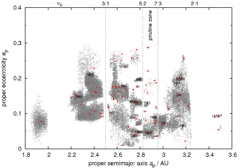
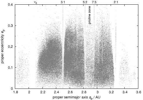
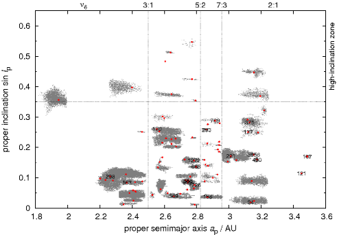
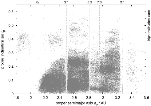
Figure 1: Asteroids from the synthetic AstDyS catalogue plotted in the proper semimajor axis $a_{\rm p}$ vs proper eccentricity $e_{\rm p}$ (top panels) and $a_{\rm p}$ vs proper inclination $\sin I_{\rm p}$ planes (bottom panels). We show the identified asteroid families (left panels) with the positions of the largest members indicated by red symbols, and also remaining background objects (right panels). The labels correspond to designations of the asteroid families that we focus on in this paper. There are still some structures consisting of small objects in the background population, visible only in the inclinations (bottom right panel). These “halos” may arise for two reasons: i) a family has no sharp boundary and its transition to the background is smooth, or ii) there are bodies escaping from the families due to long-term dynamical evolution. Nevertheless, we checked that these halo objects do not significantly affect our estimates of parent-body sizes.

There are, however, several potential problems we are aware of:

1. There may be inconsistencies among different lists of families. For example, sometimes a clump may be regarded as a single family or as two separate families. This may be the case of: Padua and Lydia, Rafita and Cameron.

2. To identify families we used synthetic proper elements, which are more precise than the semi-analytic ones. Sometimes the families look more regular (e.g., Teutonia) or more tightly clustered (Beagle) when we use the synthetic elements. This very choice may, however, affect results substantially! A clear example is the Teutonia family, which also contains the big asteroid (5) Astraea if the synthetic proper elements are used, but not if the semi-analytic proper elements are used. This is due to the large differences between the semi-analytic and synthetic proper elements of (5) Astraea. Consequently, the physical properties of the two families differ considerably. We believe that the family defined from the synthetic elements is more reliable.

3. Durda et al. (2007) often claim a larger size for the parent body (e.g., Themis, Meliboea, Maria, Eos, Gefion), because they try to match the SFD of larger bodies and the results of SPH experiments. This way they also account for small bodies that existed at the time of the disruption, but which do not exist today since they were lost due to collisional grinding and the Yarkovsky effect. We prefer to use $D_{\rm Durda}$ instead of the value $D_{\rm PB}$ estimated from the currently observed SFD. The geometric method of Tanga et al. (1999), which uses the sum of the diameters of the first and third largest family members as a first guess of the parent-body size, is essentially similar to our approach.

A complete list of all families’ members is available at our web site http://sirrah.troja.mff.cuni.cz/~mira/mp/fams/, including supporting figures.

1

Table 1: A list of asteroid families and their physical parameters. There are the following columns: $v_{\rm cutoff}$ is the selected cut–off velocity for the hierarchical clustering, $N$ the corresponding number of family members, $p_{V}$ the adopted value of the geometric albedo for family members which do not have measured diameters (from Tedesco et al. 2002 or Masiero et al. 2011, a letter ’w’ indicates it was necessary to use the WISE data to obtain median/mean albedo), taxonomic classification (according to the Sloan DSS MOC 4 colours, Parker et al. 2008), $D_{\rm PB}$ parent body size, an additional ’c’ letter indicates that we prolonged the SFD slope down to zero $D$ (a typical uncertainty is 10 %), $D_{\rm Durda}$ PB size inferred from SPH simulations (Durda et al. 2007), an exclamation mark denotes a significant mismatch with $D_{\rm PB}$, LR/PB the ratio of the volumes of the largest remnant to the parent body (an uncertainty corresponds to the last figure, a range is given if both $D_{\rm PB}$ and $D_{\rm Durda}$ are known), $v_{\rm esc}$ the escape velocity, $q_{1}$ the slope of the SFD for larger $D$, $q_{2}$ the slope for smaller $D$ (a typical uncertainty of the slopes is 0.2, if not indicated otherwise), dynamical age including its uncertainty.

designation		$v_{\rm cutoff}$	$N$	$p_{V}$	tax.	$D_{\rm PB}$	$D_{\rm Durda}$	LR/PB	$v_{\rm esc}$	$q_{1}$	$q_{2}$	age	notes, references
		m/s				km	km		m/s			Gyr
3	Juno	50	449	0.250	S	233	?	0.999	139	$-4.9$	$-3.2$	$<$0.7	cratering, Nesvorný et al. (2005)
4	Vesta	60	11169	0.351w	V	530	425!	0.995	314	$-4.5$	$-2.9$	$1.0\pm 0.25$	cratering, Marchi et al. (2012)
8	Flora	60	5284	0.304w	S	150c	160	0.81-0.68	88	$-3.4$	$-2.9$	$1.0\pm 0.5$	cut by $\nu_{6}$ resonance, LL chondrites
10	Hygiea	70	3122	0.055	C,B	410	442	0.976-0.78	243	$-4.2$	$-3.2$	$2.0\pm 1.0$	LHB? cratering
15	Eunomia	50	2867	0.187	S	259	292	0.958-0.66	153	$-5.6$	$-2.3$	$2.5\pm 0.5$	LHB? Michel et al. (2002)
20	Massalia	40	2980	0.215	S	146	144	0.995	86	$-5.0$	$-3.0$	$0.3\pm 0.1$
24	Themis	70	3581	0.066	C	268c	380-430!	0.43-0.09	158	$-2.7$	$-2.4$	$2.5\pm 1.0$	LHB?
44	Nysa (Polana)	60	9957	0.278w	S	81c	?	0.65	48	$-6.9$	$-2.6$(0.5)	$<$1.5	overlaps with the Polana family
46	Hestia	65	95	0.053	S	124	153	0.992-0.53	74	$-3.3$	$-2.0$	$<$0.2	cratering, close to J3/1 resonance
87	Sylvia	110	71	0.045	C/X	261	272	0.994-0.88	154	$-5.2$	$-2.4$	1.0-3.8	LHB? cratering, Vokrouhlický et al. (2010)
128	Nemesis	60	654	0.052	C	189	197	0.987-0.87	112	$-3.4$	$-3.3$	$0.2\pm 0.1$
137	Meliboea	95	199	0.054	C	174c	240-290!	0.59-0.20	102	$-1.9$	$-1.8$	$<$3.0	old?
142	Polana (Nysa)	60	3443	0.055w	C	75	?	0.42	45	$-7.0$	$-3.6$	$<$1.5	overlaps with Nysa
145	Adeona	50	1161	0.065	C	171c	185	0.69-0.54	101	$-5.2$	$-2.8$	$0.7\pm 0.5$	cut by J5/2 resonance
158	Koronis	50	4225	0.147	S	122c	170-180	0.024-0.009	68	$-3.6(0.3)$	$-2.3$	$2.5\pm 1.0$	LHB?
163	Erigone	60	1059	0.056	C/X	79	114	0.79-0.26	46	?	$-3.6$	$0.3\pm 0.2$
170	Maria	80	3094	0.249w	S	107c	120-130	0.070-0.048	63	$-2.5(0.3)$	$-2.8$	$3.0\pm 1.0$	LHB?
221	Eos	50	5976	0.130	K	208c	381!	0.13-0.020	123	$-3.5$	$-2.1$	$1.3\pm 0.2$
283	Emma	75	345	0.050	-	152	185	0.92-0.51	90	?	$-3.2$	$<$1.0	satellite
293	Brasilia	60	282	0.175w	C/X	34	?	0.020	20	$-1.4(0.5)$	$-3.7$	$0.05\pm 0.04$	(293) is interloper
363	Padua (Lydia)	50	596	0.097	C/X	76	106	0.045-0.017	45	$-1.8$	$-3.0$	$0.3\pm 0.2$
396	Aeolia	20	124	0.171	C/X	35	39	0.966-0.70	20	?	$-4.3$	$<$0.1	cratering
410	Chloris	90	259	0.057	C	126c	154	0.952-0.52	74	?	$-2.1$	$0.7\pm 0.4$
490	Veritas	-	-	-	C,P,D	-	100-177	-	-	-	-	$0.0083\pm 0.0005$	(490) is likely interloper (Michel et al. 2011)
569	Misa	70	543	0.031	C	88c	117	0.58-0.25	52	$-3.9$	$-2.3$	$0.5\pm 0.2$
606	Brangane	30	81	0.102	S	37	46	0.92-0.48	22	?	$-3.8$	$0.05\pm 0.04$
668	Dora	50	837	0.054	C	85	165!	0.031-0.004	50	$-4.2$	$-1.9$	$0.5\pm 0.2$
808	Merxia	50	549	0.227	S	37	121!	0.66-0.018	22	$-2.7$	$-3.4$	$0.3\pm 0.2$
832	Karin	-	-	-	S	-	40	-	-	-	-	$0.0058\pm 0.0002$
845	Naema	30	173	0.081	C	77c	81	0.35-0.30	46	$-5.2$	$-2.9$	$0.1\pm 0.05$
847	Agnia	40	1077	0.177	S	39	61	0.38-0.10	23	$-2.8$	$-3.1$	$0.2\pm 0.1$
1128	Astrid	50	265	0.079	C	43c	?	0.52	25	$-1.7$	$-2.6$	$0.1\pm 0.05$
1272	Gefion	60	19477	0.20	S	74c	100-150!	0.001-0.004	60	$-4.3$	$-2.5$	$0.48\pm 0.05$	Nesvorný et al. (2009), L chondrites
1400	Tirela	80	1001	0.070	S	86	-	0.12	86	$-4.2$	$-3.4$	$<$1.0
1658	Innes	70	621	0.246w	S	27	?	0.14	16	$-4.9$	$-3.5$	$<$0.7	(1644) Rafita is interloper
1726	Hoffmeister	40	822	0.035	C	93c	134	0.022-0.007	55	$-4.5$	$-2.7$	$0.3\pm 0.2$
3556	Lixiaohua	60	439	0.044w	C/X	62	220!	0.029-0.001	35	$-6.1$	$-3.3$	$0.15\pm 0.05$	Novaković et al. (2010)
3815	Konig	60	177	0.044	C	33	?	0.32	20	?	$-3.0$	$<$0.1	(1639) Bower is interloper
4652	Iannini	-	-	-	S	-	-	-	-	-	-	$0.005\pm 0.005$
9506	Telramund	40	146	0.217w	S	22	-	0.05	13	$-3.9$	$-3.7$	$<$0.5
18405	1993 FY12	50	44	0.171w	C/X	15	-	0.23	15	$-2.4$	$-2.4$	$<$0.2	cut by J5/2 resonance

2

Table 2: Continuation of Table 1.

designation		$v_{\rm cutoff}$	$N$	$p_{V}$	tax.	$D_{\rm PB}$	$D_{\rm Durda}$	LR/PB	$v_{\rm esc}$	$q_{1}$	$q_{2}$	age	notes, references
		m/s				km	km		m/s			Gyr
158	Koronis(2)	-	-	-	S	35	-	-	-	-	-	$0.015\pm 0.005$	cratering, Molnar & Haegert (2009)
298	Baptistina	50	1249	0.160w	C/X	35c	-	0.17	21	$-3.6$	$-2.4$	$<$0.3	part of the Flora family
434	Hungaria	200	4598	0.35	E	25	-	0.15	15	$-5.9$	$-3.1$	$0.5\pm 0.2$	Warner et al. (2010)
627	Charis	80	235	0.081	S	$>$60	-	0.53	35	?	$-3.4$	$<$1.0
778	Theobalda	85	154	0.060	C	97c	-	0.29	57	?	$-2.9$	$0.007\pm 0.002$	cratering, Novaković (2010)
302	Clarissa	30	75	0.054	C	39	-	0.96	23	?	$-3.1$	$<$0.1	cratering, Nesvorný (2010)
656	Beagle	24	63	0.089	C	64	-	0.56	38	$-1.3$	$-1.4$	$<$0.2
752	Sulamitis	60	191	0.042	C	65	-	0.83	39	$-6.5$	$-2.3$	$<$0.4
1189	Terentia	50	18	0.070	C	56	-	0.990	33	?	$-2.6$?	$<$0.2	cratering
1892	Lucienne	100	57	0.223w	S	14	-	0.71	8	?	$-4.4$	$<$0.3
7353	Kazvia	50	23	0.206w	S	16	-	0.57	8	?	$-1.8$	$<$0.1
10811	Lau	100	15	0.273w	S	11	-	0.77	5	?	$-2.8$	$<$0.1
18466	1995 SU37	40	71	0.241w	S	14	-	0.045	7	?	$-5.0$	$<$0.3
1270	Datura	-	-	-	S	-	-	-	-	-	-	0.00045-0.00060	identified in osculating-element space,
14627	Emilkowalski	-	-	-	C/X	-	-	-	-	-	-	0.00019-0.00025	Nesvorný & Vokrouhlický (2006)
16598	1992 YC2	-	-	-	S	-	-	-	-	-	-	0.00005-0.00025
21509	Lucascavin	-	-	-	S	-	-	-	-	-	-	0.0003-0.0008
2384	Schulhof	-	-	-	S	-	-	-	-	-	-	0.0007-0.0009	Vokrouhlický & Nesvorný (2011)
27	Euterpe	70	268	0.260w	S	118c	-	0.998	70	$-2.9$	$-2.2$	$<$1.0	cratering, Parker et al. (2008)
375	Ursula	80	777	0.057w	C	203c	240-280	0.71-0.43	120	$-4.1$	$-2.3$	$<$3.5	old?
1044	Teutonia	50	1950	0.343	S	27-120	-	0.17-0.98	16-71	$-3.5$	$-3.9$	$<$0.5	depends on (5) Astraea membership
1296	Andree	60	401	0.290w	S	17-74	-	0.010-0.95	10-43	?	$-2.9(0.5)$	$<$1.0	depends on (79) Eurynome membership
2007	McCuskey	34	236	0.06	C	29	-	0.41	17	?	$-5.6$	$<$0.5	overlaps with Nysa/Polana
2085	Henan	54	946	0.200w	S	27	-	0.13	16	$-4.2$	$-3.2$	$<$1.0
2262	Mitidika	83	410	0.064w	C	49-79c	-	0.037-0.81	26-46	$-4.5$	$-2.2$	$<$1.0	depends on (785) Zwetana membership, (2262) is interloper, overlaps with Juno
2	Pallas	200	64	0.163	B	498c	-	0.9996	295	?	$-2.2$	$<$0.5	high-$I$, Carruba (2010)
25	Phocaea	160	1370	0.22	S	92	-	0.54	55	$-3.1$	$-2.4$	$<$2.2	old? high-$I/e$, cut by $\nu_{6}$ resonance, Carruba (2009)
148	Gallia	150	57	0.169	S	98	-	0.058	58	?	$-3.6$	$<$0.45	high-$I$
480	Hansa	150	651	0.256	S	60	-	0.83	35	$-4.9$	$-3.2$	$<$1.6	high-$I$
686	Gersuind	130	178	0.146	S	52c	-	0.48	40	?	$-2.7$	$<$0.8	high-$I$, Gil-Hutton (2006)
945	Barcelona	110	129	0.248	S	28	-	0.77	16	?	$-3.5$	$<$0.35	high-$I$, Foglia & Masi (2004)
1222	Tina	110	37	0.338	S	21	-	0.94	12	?	$-4.1$	$<$0.15	high-$I$
4203	Brucato	-	-	-	-	-	-	-	-	-	-	$<$1.3	in freq. space
31	Euphrosyne	100	851	0.056	C	259	-	0.97	153	$-4.9$	$-3.9$	$<$1.5	cratering, high-$I$, Foglia & Massi (2004)
702	Alauda	120	791	0.070	B	218c	290-330!	0.025	129	$-3.9$	$-2.4$	$<$3.5	old? high-$I$, cut by J2/1 resonance, satellite (Margot & Rojo 2007)
107	Camilla	?	?	0.054	-	$>$226	?	?	?	?	?	3.8?	LHB? Cybele region, non-existent today,
121	Hermione	?	?	0.058	-	$>$209	?	?	?	?	?	3.8?	LHB? Vokrouhlický et al. (2010)

3

Table 3: Continuation of Table 1.

designation		$v_{\rm cutoff}$	$N$	$p_{V}$	tax.	$D_{\rm PB}$	$D_{\rm Durda}$	LR/PB	$v_{\rm esc}$	$q_{1}$	$q_{2}$	age	notes, references
		m/s				km	km		m/s			Gyr
1303	Luthera	100	142	0.043	X	92	-	0.81	54	$-3.9$	$-2.7$	$<$0.5	above (375) Ursula
1547	Nele	20	57	0.311w	X	19	-	0.85	11	?	$-2.8(0.3)$	$<$0.04	close to (3) Juno
2732	Witt	60	985	0.260w	S	25	-	0.082	15	$-4.0(0.3)$	$-3.8$	$<$1.0	only part with $\sin I>0.099$, above (363) Padua
81	Terpsichore	120	70	0.052	C	119	-	0.993	71	?	$-4.4$	$<$0.5	cratering, less-certain families in the “pristine zone”
709	Fringilla	140	60	0.047	X	99c	130-140	0.93-0.41	59	$-6.2$	$-1.7$	$<$2.5	old?
918	Itha	140	63	0.23	S	38	-	0.16	22	$-2.7$	$-1.5$	$<$1.5	shallow SFD
5567	Durisen	100	18	0.044w	X	42	-	0.89	25	?	$-1.7$	$<$0.5	shallow SFD
5614	Yakovlev	100	34	0.05	C	22	-	0.28	13	?	$-3.2$	$<$0.2
12573	1999 NJ53	40	13	0.190w	C	15	-	0.13	9	?	$-2.0(0.5)$	$<$0.6	incomplete SFD
15454	1998 YB3	50	14	0.054w	C	21	-	0.41	13	?	$-1.6(0.3)$	$<$0.5	shallow SFD
15477	1999 CG1	110	144	0.098w	S	25	-	0.065	14	?	$-4.6(0.5)$	$<$1.5
36256	1999 XT17	60	30	0.210w	S	17	-	0.037	10	?	$-1.4(0.5)$	$<$0.3	shallow SFD

2.1 A definition of the production function

To compare observed families to simulations, we define a “production function” as the cumulative number $N({>}D)$ of families with parent-body size $D_{\rm PB}$ larger than a given $D$. The observed production function is shown in Figure 2, and it is worth noting that it is very shallow. The number of families with $D_{\rm PB}\simeq 100\,{\rm km}$ is comparable to the number of families in the $D_{\rm PB}=200$–400 km range.

It is important to note that the observed production function is likely to be affected by biases (the family sample may not be complete, especially below $D_{\rm PB}\lesssim 100\,{\rm km}$) and also by long-term collisional/dynamical evolution which may prevent a detection of old comminutioned/dispersed families today (Marzari et al. 1999).

From the theoretical point of view, the slope $q$ of the production function $N({>}D)\propto D^{q}$ should correspond to the cumulative slopes of the size-frequency distributions of the target and projectile populations. It is easy to show that the relation is

$$q=2+q_{\rm target}+{5\over 3}q_{\rm project}\,.$$ (1)

Of course, real populations may have complicated SFDs, with different slopes in different ranges. Nevertheless, any populations that have a steep SFD (e.g. $q_{\rm target}=q_{\rm project}=-2.5$) would inevitably produce a steep production function ($q\doteq-4.7$).

In the following analysis, we drop cratering events and discuss catastrophic disruptions only, i.e. families which have largest remnant/parent body mass ratio less than 0.5. The reason is that the same criterion ${\rm LR}/{\rm PB}<0.5$ is used in collisional models. Moreover, cratering events were not yet systematically explored by SPH simulations due to insufficient resolution (Durda et al. 2007).

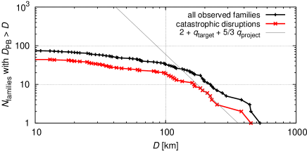
Figure 2: A production function (i.e. the cumulative number $N({>}D)$ of families with parent-body size $D_{\rm PB}$ larger than $D$) for all observed families (black) and families corresponding to catastrophic disruptions (red), i.e. with largest remnant/parent body mass ratio lower than 0.5. We also plot a theoretical slope according to Eq. (1), assuming $q_{\rm target}=-3.2$ and $q_{\rm project}=-1.2$, which correspond to the slopes of the main belt population in the range $D=100$–200 km and $D=15$–60 km, respectively.

2.2 Methods for family age determination

If there is no previous estimate of the age of a family, we used one of the following three dynamical methods to determine it: i) a simple $(a_{\rm p},H)$ analysis as in Nesvorný et al. (2005); ii) a $C$-parameter distribution fitting as introduced by Vokrouhlický et al. (2006); iii) a full N-body simulation described e.g. in Brož et al. (2011).

In the first approach, we assume zero initial velocities, and the current extent of the family is explained by the size-dependent Yarkovsky semimajor axis drift. This way we can obtain only an upper limit for the dynamical age, of course. We show an example for the Eos family in Figure 3. The extent of the family in the proper semimajor axis vs the absolute magnitude $(a_{\rm p},H)$ plane can be described by the parametric relation

$$0.2H=\log_{10}{|a_{\rm p}-a_{\rm c}|\over C}\,,$$ (2)

where $a_{\rm c}$ denotes the centre of the family, and $C$ is the parameter. Such relation can be naturally expected when the semimajor-axis drift rate is inversely proportional to the size, ${{\rm d}a/{\rm d}t}\propto 1/D$, and the size is related to the absolute magnitude via the Pogson equation $H=-2.5\log_{10}(p_{V}D^{2}/D_{0}^{2})$, where $D_{0}$ denotes the reference diameter and $p_{V}$ the geometric albedo (see Vokrouhlický et al. 2006 for a detailed discussion). The limiting value, for which all Eos family members (except interlopers) are above the corresponding curve, is $C=1.5\hbox{ to }2.0\times 10^{-4}\,{\rm AU}$. Assuming reasonable thermal parameters (summarised in Table 4), we calculate the expected Yarkovsky drift rates ${{\rm d}a/{\rm d}t}$ (using the theory from Brož 2006) and consequently can determine the age to be $t<1.5\hbox{ to }2.0\,{\rm Gyr}$.

The second method uses a histogram $N(C,C+\Delta C)$ of the number of asteroids with respect to the $C$ parameter defined above, which is fitted by a dynamical model of the initial velocity field and the Yarkovsky/YORP evolution. This enables us to determine the lower limit for the age too (so the resulting age estimate is $t=1.3^{+0.15}_{-0.2}\,{\rm Gyr}$ for the Eos family).

In the third case, we start an N-body simulation using a modified SWIFT integrator (Levison and Duncan 1994), with the Yarkovsky/YORP acceleration included, and evolve a synthetic family up to 4 Gyr. We try to match the shape of the observed family in all three proper orbital elements $(a_{\rm p},e_{\rm p},\sin I_{\rm p})$. In principle, this method may provide a somewhat independent estimate of the age. For example, there is a ‘halo’ of asteroids in the surroundings of the nominal Eos family, which are of the same taxonomic type K, and we may fit the ratio $N_{\rm halo}/N_{\rm core}$ of the number of objects in the ‘halo’ and in the family ‘core’ (Brož et al., in preparation).

The major source of uncertainty in all methods are unknown bulk densities of asteroids (although we use the most likely values for the S or C/X taxonomic classes, Carry 2012). The age scales approximately as $t\propto\rho_{\rm bulk}$. Nevertheless, we are still able to distinguish families that are young from those that are old, because the allowed ranges of densities for S-types ($2\hbox{ to }3\,{\rm g}/{\rm cm}^{3}$) and C/X-types ($1\hbox{ to }2\,{\rm g}/{\rm cm}^{3}$) are limited (Carry 2012) and so are the allowed ages of families.

Table 4: Nominal thermal parameters for S and C/X taxonomic types of asteroids: $\rho_{\rm bulk}$ denotes the bulk density, $\rho_{\rm surf}$ the surface density, $K$ the thermal conductivity, $C_{\rm th}$ the specific thermal capacity, $A_{\rm Bond}$ the Bond albedo and $\epsilon$ the infrared emissivity.

type	$\rho_{\rm bulk}$	$\rho_{\rm surf}$	$K$	$C_{\rm th}$	$A_{\rm Bond}$	$\epsilon$
	(${\rm kg}/{\rm m}^{3}$)	(${\rm kg}/{\rm m}^{3}$)	(${\rm W}/{\rm m}/{\rm K}$)	(${\rm J}/{\rm kg}/{\rm K}$)
S	2500	1500	0.001	680	0.1	0.9
C/X	1300	1300	0.01	680	0.02	0.9

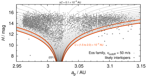
Figure 3: An example of the Eos asteroid family, shown on the proper semimajor axis $a_{\rm p}$ vs absolute magnitude $H$ plot. We also plot curves defined by equation (2) and parameters $a_{\rm c}=3.019\,{\rm AU}$, $C=1.5\hbox{ to }2.0\times 10^{-4}\,{\rm AU}$, which is related to the upper limit of the dynamical age of the family.

2.3 Which families can be of LHB origin?

The ages of the observed families and their parent-body sizes are shown in Figure 4. Because the ages are generally very uncertain, we consider that any family whose nominal age is older than 2 Gyr is potentially a family formed ${\sim}4$ Gyr ago, i.e. at the LHB time. If we compare the number of “young” (${<}2\,{\rm Gyr}$) and old families (${>}2\,{\rm Gyr}$) with $D_{\rm PB}=200$–400 km, we cannot see a significant over-abundance of old family formation events. On the other hand, we almost do not find any small old families.

Only 12 families from the whole list may be possibly dated back to the late heavy bombardment, because their dynamical ages approach $\sim 3.8\,{\rm Gyr}$ (including the relatively large uncertainties; see Table 5, which is an excerpt from Tables 1–3).

If we drop cratering events and the families of Camilla and Hermione, which do not exist any more today (their existence was inferred from the satellite systems, Vokrouhlický et al. 2010), we end up with only five families created by catastrophic disruptions that may potentially date from the LHB time (i.e. their nominal age is more than 2 Gy). As we shall see in Section 4, this is an unexpectedly low number.

Moreover, it is really intriguing that most “possibly-LHB” families are larger than $D_{\rm PB}\simeq 200\,{\rm km}$. It seems that old families with $D_{\rm PB}\simeq 100\,{\rm km}$ are missing in the observed sample. This is an important aspect that we have to explain, because it contradicts our expectation of a steep production function.

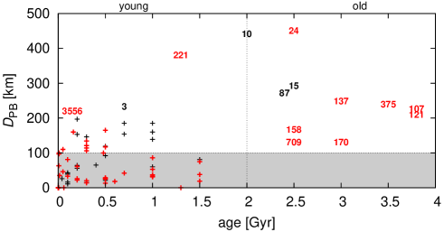
Figure 4: The relation between dynamical ages of families and the sizes of their parent bodies. Red labels correspond to catastrophic disruptions, while cratering events are labelled in black. Some of the families are denoted by the designation of the largest member. The uncertainties of both parameters are listed in Tables 1–3 (we do not include overlapping error bars here for clarity).

Table 5: Old families with ages possibly approaching the LHB. They are sorted according to the parent body size, where $D_{\rm Durda}$ determined by the Durda et al. (2007) method is preferred to the estimate $D_{\rm PB}$ inferred from the observed SFD. An additional ‘c’ letter indicates that we extrapolated the SFD down to $D=0\,{\rm km}$ to account for small (unobserved) asteroids, an exclamation mark denotes a significant mismatch between $D_{\rm PB}$ and $D_{\rm Durda}$.

designation		$D_{\rm PB}$	$D_{\rm Durda}$	note
		(km)	(km)
24	Themis	209c	380–430!
10	Hygiea	410	442	cratering
15	Eunomia	259	292	cratering
702	Alauda	218c	290–330!	high-$I$
87	Sylvia	261	272	cratering
137	Meliboea	174c	240–290!
375	Ursula	198	240–280	cratering
107	Camilla	$>$226	-	non-existent
121	Hermione	$>$209	-	non-existent
158	Koronis	122c	170–180
709	Fringilla	99c	130–140	cratering
170	Maria	100c	120–130

3 Collisions in the main belt alone

Before we proceed to scenarios involving the LHB, we try to explain the observed families with ages spanning 0–4 Gyr as a result of collisions only among main-belt bodies. To this purpose, we used the collisional code called Boulder (Morbidelli et al. 2009) with the following setup: the intrinsic probabilities $P_{\rm i}=3.1\times 10^{-18}\,{\rm km}^{-2}\,{\rm yr}^{-1}$, and the mutual velocities $V_{\rm imp}=5.28\,{\rm km}/{\rm s}$ for the MB vs MB collisions (both were taken from the work of Dahlgren 1998). The assumption of a single $V_{\rm imp}$ value is a simplification, but about 90 % collisions have mutual velocities between $2\hbox{ and }8\,{\rm km}/{\rm s}$ (Dahlgren 1998), which assures a similar collisional regime.

The scaling law is described by the polynomial relation ($r$ denotes radius in cm)

$$Q^{\star}_{D}(r)={1\over q_{\rm fact}}\left(Q_{0}r^{a}+B\rho r^{b}\right)$$ (3)

with the parameters corresponding to basaltic material at 5 km/s (Benz & Asphaug 1999):

$\rho$	$Q_{0}$	$a$	$B$	$b$	$q_{\rm fact}$
$({\rm g}/{\rm cm}^{3})\!\!\!$	$\!\!({\rm erg}/{\rm g})\!\!$		$\!\!\!({\rm erg}/{\rm g})\!\!\!$
3.0	$7\times 10^{7}$	$-0.45$	2.1	1.19	1.0

Even though not all asteroids are basaltic, we use the scaling law above as a mean one for the main-belt population. Below, we discuss also the case of significantly lower strengths (i.e. higher $q_{\rm fact}$ values).

We selected the time span of the simulation 4 Gyr (not 4.5 Gyr) since we are interested in this last evolutionary phase of the main belt, when its population and collisional activity is nearly same as today (Bottke et al. 2005). The outcome of a single simulation also depends on the “seed” value of the random-number generator that is used in the Boulder code to decide whether a collision with a fractional probability actually occurs or not in a given time step. We thus have to run multiple simulations (usually 100) to obtain information on this stochasticity of the collisional evolution process.

The initial SFD of the main belt population conditions was approximated by a three-segment power law (see also thin grey line in Figure 5, 1st row) with differential slopes $q_{a}=-4.3$ (for $D>D_{1}$), $q_{b}=-2.2$, $q_{c}=-3.5$ (for $D<D_{2}$) where the size ranges were delimited by $D_{1}=80\,{\rm km}$ and $D_{2}=16\,{\rm km}$. We also added a few big bodies to reflect the observed shape of the SFD at large sizes ($D>400\,{\rm km}$). The normalisation was $N_{\rm norm}(D>D_{1})=350$ bodies in this case.

We used the observed SFD of the main belt as the first constraint for our collisional model. We verified that the outcome our model after 4 Gyr is not sensitive to the value of $q_{c}$. Namely, a change of $q_{c}$ by as much as $\pm 1$ does not affect the final SFD in any significant way. On the other hand, the values of the remaining parameters ($q_{a}$, $q_{b}$, $D_{1}$, $D_{2}$, $N_{\rm norm}$) are enforced by the observed SFD. To obtain a reasonable fit, they cannot differ much (by more than 5–10 %) from the values presented above.

We do not use only a single number to describe the number of observed families (e.g. $N=20$ for $D_{\rm PB}\geq 100\,{\rm km}$), but we discuss a complete production function instead. The results in terms of the production function are shown in Figure 5 (left column, 2nd row). On average, the synthetic production function is steeper and below the observed one, even though there is approximately a 5 % chance that a single realization of the computer model will resemble the observations quite well. This also holds for the distribution of $D_{\rm PB}=200$–400 km families in the course of time (age).

In this case, the synthetic production function of $D_{\rm PB}\gtrsim 100\,{\rm km}$ families is not significantly affected by comminution. According to Bottke et al. (2005), most of $D>10\,{\rm km}$ fragments survive intact and a $D_{\rm PB}\gtrsim 100\,{\rm km}$ family should be recognisable today. This is also confirmed by calculations with Boulder (see Figure 5, left column, 3rd row).

To improve the match between the synthetic and the observed production function, we can do the following: i) modify the scaling law, or ii) account for a dynamical decay of the MB population. Using a substantially lower strength ($q_{\rm fact}=5$ in Eq. (3), which is not likely, though) one can obtain a synthetic production function which is on average consistent with the observations in the $D_{\rm PB}=200$–400 km range.

Regarding the dynamical decay, Minton & Malhotra (2010) suggest that initially the MB was three times more populous than today while the decay timescale was very short: after 100 Myr of evolution the number of bodies is almost at the current level. In this brief period of time, about 50 % more families will be created, but all of them will be old, of course. For the remaining $\sim 3.9\,{\rm Gyr}$, the above model (without any dynamical decay) is valid.

To conclude, it is possible – though not very likely – that the observed families were produced by the collisional activity in the main belt alone. A dynamical decay of the MB population would create more families that are old, but technically speaking, this cannot be distinguished from the LHB scenario, which is discussed next.

MB alone	MB vs comets	MB vs disrupting comets

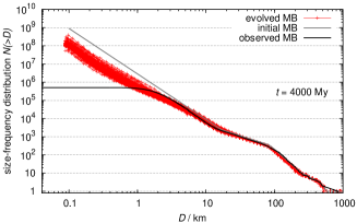
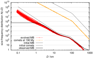
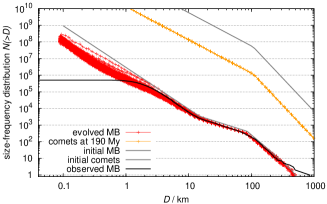
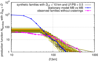
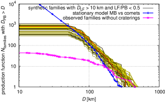
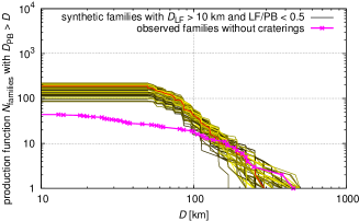
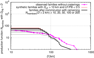
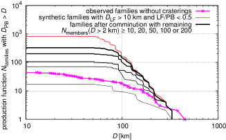
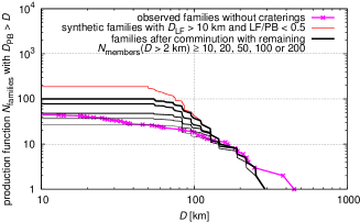
Figure 5: Results of three different collisional models: main-belt alone which is discussed in Section 3 (left column), main-belt and comets from Section 4 (middle column), main-belt and disrupting comets from Section 7 (right column). 1st row: the initial and evolved size-frequency distributions of the main belt populations for 100 Boulder simulations; 2nd row: the resulting family production functions (in order to distinguish 100 lines we plot them using different colours ranging from black to yellow) and their comparison to the observations; 3rd row: the production function affected by comminution for a selected simulation; and 4th row: the distribution of synthetic families with $D_{\rm PB}\geq 50\,{\rm km}$ in the (age, $D_{\rm PB}$) plot for a selected simulation, without comminution. The positions of synthetic families in the 4th-row figures may differ significantly for a different Boulder simulation due to stochasticity and low-number statistics. Moreover, in the middle and right columns, many families were created during the LHB, so there are many overlapping crosses close to $4\,{\rm Gyr}$.

4 Collisions between a “classical” cometary disk and the main belt

In this section, we construct a collisional model and estimate an expected number of families created during the LHB due to collisions between cometary-disk bodies and main-belt asteroids. We start with a simple stationary model and we confirm the results using a more sophisticated Boulder code (Morbidelli et al. 2009).

Using the data from Vokrouhlický et al. (2008) for a “classical” cometary disk, we can estimate the intrinsic collisional probability and the collisional velocity between comets and asteroids. A typical time-dependent evolution of $P_{\rm i}$ and $V_{\rm imp}$ is shown in Figure 6. The probabilities increase at first, as the transneptunian cometary disk starts to decay, reaching up to $6\times 10^{-21}\,{\rm km}^{-2}\,{\rm yr}^{-1}$, and after $100\,{\rm Myr}$ they decrease to zero. These results do not differ significantly from run to run.

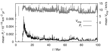
Figure 6: The temporal evolution of the intrinsic collisional probability $P_{\rm i}$ (bottom) and mean collisional velocity $V_{\rm imp}$ (top) computed for collisions between cometary-disk bodies and the main-belt asteroids. The time $t=0$ is arbitrary here; the sudden increase in $P_{i}$ values corresponds to the beginning of the LHB.

4.1 Simple stationary model

In a stationary collisional model, we choose an SFD for the cometary disk, we assume a current population of the main belt; estimate the projectile size needed to disrupt a given target according to (Bottke et al. 2005)

$$d_{\rm disrupt}=\left({2Q^{\star}_{D}/V_{\rm imp}^{2}}\right)^{1/3}D_{\rm target}\,,$$ (4)

where $Q^{\star}_{D}$ denotes the specific energy for disruption and dispersion of the target (Benz & Asphaug 1999); and finally calculate the number of events during the LHB as

$$n_{\rm events}={D_{\rm target}^{2}\over 4}\,n_{\rm target}\int P_{i}(t)\,n_{\rm project}(t)\,{\rm d}t\,,$$ (5)

where $n_{\rm target}$ and $n_{\rm project}$ are the number of targets (i.e. main belt asteroids) and the number of projectiles (comets), respectively. The actual number of bodies (27,000) in the dynamical simulation of Vokrouhlický et al. (2008) changes in the course of time, and it was scaled such that it was initially equal to the number of projectiles $N({>}d_{\rm disrupt})$ inferred from the SFD of the disk. This is clearly a lower limit for the number of families created, since the main belt was definitely more populous in the past.

The average impact velocity is $V_{\rm imp}\simeq 10\,{\rm km}/{\rm s}$, so we need the following projectile sizes to disrupt given target sizes:

$D_{\rm target}$	$N_{\rm targets}$	$Q^{\star}_{D}$	$d_{\rm disrupt}$ for ${\rho_{\rm target}\over\rho_{\rm project}}=3\hbox{ to }6$
(km)	in the MB	(J/kg)	(km)
100	$\sim$192	$1\times 10^{5}$	12.6 to 23
200	$\sim$23	$4\times 10^{5}$	40.0 to 73

We tried to use various SFDs for the cometary disk (i.e., with various differential slopes $q_{1}$ for $D>D_{0}$ and $q_{2}$ for $D<D_{0}$, the elbow diameter $D_{0}$ and total mass $M_{\rm disk}$), including rather extreme cases (see Figure 7). The resulting numbers of LHB families are summarised in Table 6. Usually, we obtain several families with $D_{\rm PB}\simeq 200\,{\rm km}$ and about $100$ families with $D_{\rm PB}\simeq 100\,{\rm km}$. This result is robust with respect to the slope $q_{2}$, because even very shallow SFDs should produce a lot of these families. The only way to decrease the number of families significantly is to assume the elbow at a larger diameter $D_{0}\simeq 150\,{\rm km}$.

It is thus no problem to explain the existence of approximately five large families with $D_{\rm PB}=200$–400 km, which are indeed observed, since they can be readily produced during the LHB. On the other hand, the high number of $D_{\rm PB}\simeq 100\,{\rm km}$ families clearly contradicts the observations, since we observe almost no LHB families of this size.

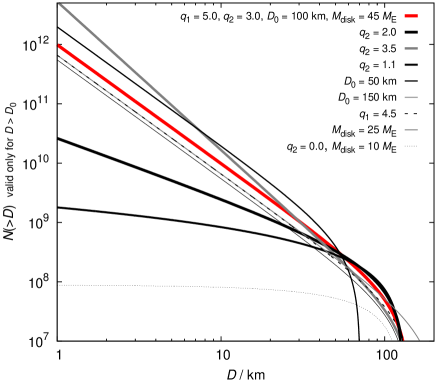
Figure 7: Cumulative size-frequency distributions of the cometary disk tested in this work. All the parameters of our nominal choice are given in the top label; the other labels just report the parameters that changed relative to our nominal choice.

Table 6: Results of a stationary collisional model between the cometary disk and the main belt. The parameters characterise the SFD of the disk: $q_{1}$, $q_{2}$ are differential slopes for the diameters larger/smaller than the elbow diameter $D_{0}$, $M_{\rm disk}$ denotes the total mass of the disk, and $n_{\rm events}$ is the resulting number of families created during the LHB for a given parent body size $D_{\rm PB}$. The ranges of $n_{\rm events}$ are due to variable density ratios $\rho_{\rm target}/\rho_{\rm project}=1\hbox{ to }3/1$.

$q_{1}$	$q_{2}$	$D_{0}$	$M_{\rm disk}$	$n_{\rm events}$			notes
		(km)	($M_{\oplus}$)	for $D_{\rm PB}\geq 100\,{\rm km}$	$D_{\rm PB}\geq 200\,{\rm km}$	Vesta craterings
5.0	3.0	100	45	115–55	4.9–2.1	2.0	nominal case
5.0	2.0	100	45	35–23	4.0–2.2	1.1	shallow SFD
5.0	3.5	100	45	174–70	4.3–1.6	1.8	steep SFD
5.0	1.1	100	45	14–12	3.1–2.1	1.1	extremely shallow SFD
4.5	3.0	100	45	77–37	3.3–1.5	1.3	lower $q_{1}$
5.0	3.0	50	45	225–104	7.2–1.7	3.2	smaller turn-off
5.0	3.0	100	25	64–40	2.7–1.5	1.1	lower $M_{\rm disk}$
5.0	3.0	100	17	34	1.2	1.9	$\rho_{\rm comets}=500\,{\rm kg}/{\rm m}^{3}$
5.0	3.0	150	45	77–23	3.4–0.95	0.74	larger turn-off
5.0	0.0	100	10	1.5–1.4	0.5–0.4	0.16	worst case (zero $q_{2}$ and low $M_{\rm disk}$)

4.2 Constraints from (4) Vesta

The asteroid (4) Vesta presents a significant constraint for collisional models, being a differentiated body with a preserved basaltic crust (Keil 2002) and a 500 km large basin on its surface (a feature indicated by the photometric analysis of Cellino et al. 1987), which is significantly younger than 4 Gyr (Marchi et al. 2012). It is highly unlikely that Vesta experienced a catastrophic disruption in the past, and even large cratering events were limited. We thus have to check the number of collisions between one $D=530$ km target and $D\simeq 35$ km projectiles, which are capable of producing the basin and the Vesta family (Thomas et al. 1997). According to Table 6, the predicted number of such events does not exceed $\sim 2$, so given the stochasticity of the results there is a significant chance that Vesta indeed experienced zero such impacts during the LHB.

4.3 Simulations with the Boulder code

To confirm results of the simple stationary model, we also performed simulations with the Boulder code. We modified the code to include a time-dependent collisional probability $P_{\rm i}(t)$ and impact velocity $V_{\rm imp}(t)$ of the cometary-disk population.

We started a simulation with a setup for the cometary disk resembling the nominal case from Table 6. The scaling law is described by Eq. (3), with the following parameters (the first set corresponds to basaltic material at 5 km/s, the second one to water ice, Benz & Asphaug 1999):

	$\rho$	$Q_{0}$	$a$	$B$	$b$	$q_{\rm fact}$
	$\!\!\!({\rm g}/{\rm cm}^{3})\!\!\!$	$\!\!({\rm erg}/{\rm g})\!\!$		$\!\!\!({\rm erg}/{\rm g})\!\!\!$
asteroids	3.0	$7\times 10^{7}$	$-0.45$	2.1	1.19	1.0
comets	1.0	$1.6\times 10^{7}$	$-0.39$	1.2	1.26	3.0

The intrinsic probabilities $P_{\rm i}=3.1\times 10^{-18}\,{\rm km}^{-2}\,{\rm yr}^{-1}$ and velocities $V_{\rm imp}=5.28\,{\rm km}/{\rm s}$ for the MB vs MB collisions were again taken from the work of Dahlgren (1998). We do not account for comet–comet collisions since their evolution is dominated by the dynamical decay. The initial SFD of the main belt was similar to the one in Section 3, $q_{a}=-4.2$, $q_{b}=-2.2$, $q_{c}=-3.5$, $D_{1}=80\,{\rm km}$, $D_{2}=14\,{\rm km}$, and only the normalisation was increased up to $N_{\rm norm}(D>D_{1})=560$ in this case.

The resulting size-frequency distributions of 100 independent simulations with different random seeds are shown in Figure 5 (middle column). The number of LHB families (approximately 10 with $D_{\rm PB}\simeq 200\,{\rm km}$ and 200 with $D_{\rm PB}\simeq 100\,{\rm km}$) is even larger compared to the stationary model, as expected, because we had to start with a larger main belt to get a good fit of the currently observed MB after 4 Gyr of collisional evolution.

To conclude, the stationary model and the Boulder code give results that are compatible with each other, but that clearly contradict the observed production function of families. In particular, they predict far too many families with $D=100$ km parent bodies. At first sight, this may be interpreted as proof that there was no cometary LHB on the asteroids. Before jumping to this conclusion, however, one has to investigate whether there are biases against identifying of $D_{\rm PB}=100\,{\rm km}$ families. In Sections 5–9 we discuss several mechanisms that all contribute, at some level, to reducing the number of observable $D_{\rm PB}=100$ km families over time. They are addressed in order of relevance, from the least to the most effective.

5 Families overlap

Because the number of expected $D_{\rm PB}\geq 100\,{\rm km}$ LHB families is very high (of the order of $100$) we now want to verify if these families can overlap in such a way that they cannot be distinguished from each other and from the background. We thus took 192 main-belt bodies with $D\geq 100\,{\rm km}$ and selected randomly 100 of them that will break apart. For each one we created an artificial family with $10^{2}$ members, assume a size-dependent ejection velocity $V\propto 1/D$ (with $V=50\,{\rm m}/{\rm s}$ for $D=5\,{\rm km}$) and the size distribution resembling that of the Koronis family. The choice of the true anomaly and the argument of perihelion at the instant of the break-up event was random. We then calculated proper elements $(a_{\rm p},e_{\rm p},\sin I_{\rm p})$ for all bodies. This type of analysis is in some respects similar to the work of Bendjoya et al. (1993).

According to the resulting Figure 8 the answer to the question is simple: the families do not overlap sufficiently, and they cannot be hidden that way. Moreover, if we take only bigger bodies ($D>10\,{\rm km}$), these would be clustered even more tightly. The same is true for proper inclinations, which are usually more clustered than eccentricities, so families could be more easily recognised.

Figure 8: The proper semimajor axis $a_{\rm p}$ vs the proper eccentricity $e_{\rm p}$ for 100 synthetic families created in the main belt. It is the initial state, shortly after disruption events. We assume the size-frequency distribution of bodies in each synthetic family similar to that of the Koronis family (down to $D\simeq 2\,{\rm km}$). Break-ups with the true anomaly $f\simeq 0\hbox{ to }30^{\circ}$ and $150^{\circ}\hbox{ to }180^{\circ}$ are more easily visible on this plot, even though the choice of both $f$ and the argument of perihelion $\varpi$ was random for all families.

6 Dispersion of families by the Yarkovsky drift

In this section, we model long-term evolution of synthetic families driven by the Yarkovsky effect and chaotic diffusion. For one synthetic family located in the outer belt, we have performed a full N-body integration with the SWIFT package (Levison & Duncan 1994), which includes also an implementation of the Yarkovsky/YORP effect (Brož 2006) and second-order integrator by Laskar & Robutel (2001). We included 4 giant planets in this simulation. To speed-up the integration, we used ten times smaller sizes of the test particles and thus a ten times shorter time span (400 Myr instead of 4 Gyr). The selected time step is $\Delta t=91\,{\rm d}$. We computed proper elements, namely their differences $\Delta a_{\rm p},\Delta e_{\rm p},\Delta\sin I_{\rm p}$ between the initial and final positions.

Then we used a simple Monte-Carlo approach for the whole set of 100 synthetic families — we assigned a suitable drift $\Delta a_{\rm p}(D)$ in semimajor axis, and also drifts in eccentricity $\Delta e_{\rm p}$ and inclination $\Delta\sin I_{\rm p}$ to each member of 100 families, respecting asteroid sizes, of course. This way we account for the Yarkovsky semimajor axis drift and also for interactions with mean-motion and secular resonances. This Monte-Carlo method tends to smear all structures, so we can regard our results as the upper limits for dispersion of families.

While the eccentricities of small asteroids (down to $D\simeq 2\,{\rm km}$) seem to be dispersed enough to hide the families, there are still some persistent structures in inclinations, which would be observable today. Moreover, large asteroids ($D\geq 10\,{\rm km}$) seem to be clustered even after $4\,{\rm Gyr}$, so that more than 50 % of families can be easily recognised against the background (see Figure 9). We thus can conclude that it is not possible to disperse the families by the Yarkovsky effect alone.

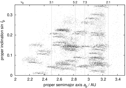
Figure 9: The proper semimajor axis $a_{\rm p}$ vs the proper inclination $\sin I_{\rm p}$ for 100 synthetic asteroid families (black dots), evolved over 4 Gyr using a Monte-Carlo model. The assumed SFDs correspond to the Koronis family, but we show only $D>10\,{\rm km}$ bodies here. We also include $D>10\,{\rm km}$ background asteroids (grey dots) for comparison.

7 Reduced physical lifetime of comets in the MB crossing zone

To illustrate the effects that the physical disruption of comets (due to volatile pressure build-up, amorphous/crystalline phase transitions, spin-up by jets, etc.) can have on the collisional evolution of the asteroid belt, we adopted here a simplistic assumption. We considered that no comet disrupt beyond 1.5 AU, whereas all comets disrupt the first time that they penetrate inside 1.5 AU. Both conditions are clearly not true in reality: some comets are observed to blow up beyond 1.5 AU, and others are seen to survive on an Earth-crossing orbit. Thus we adopted our disruption law just as an example of a drastic reduction of the number of comets with small perihelion distance, as required to explain the absence of evidence for a cometary bombardment on the Moon.

We then removed all those objects from output of comet evolution during the LHB that had a passage within 1.5 AU from the Sun, from the time of their first passage below this threshold. We then recomputed the mean intrinsic collision probability of a comet with the asteroid belt. The result is a factor $\sim$3 smaller than when no physical disruption of comets is taken into account as in Fig. 6. The mean impact velocity with asteroids also decreases, from 12 km/s to 8 km/s.

The resulting number of asteroid disruption events is thus decreased by a factor $\sim$4.5, which can be also seen in the production function shown in Figure 5 (right column). The production of families with $D_{\rm PB}=200$–400 km is consistent with observations, while the number of $D_{\rm PB}\simeq 100$ km families is reduced to 30–70, but is still too high, by a factor 2–3. More importantly, the slope of the production function remains steeper than that of the observed function. Thus, our conclusion is that physical disruptions of comets alone cannot explain the observation, but may be an important factor to keep in mind for reconciling the model with the data.

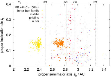
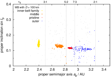
Figure 10: The proper semimajor axis vs the proper inclination for four synthetic families (distinguished by symbols) as perturbed by giant-planet migration. Left panel: the case when families were evolved over the “jump” due to the encounter between Jupiter and Neptune. Right panel: the families created just after the jump and perturbed only by later phases of migration.

8 Perturbation of families by migrating planets (a jumping-Jupiter scenario)

In principle, families created during the LHB may be perturbed by still-migrating planets. It is an open question what the exact orbital evolution of planets was at that time. Nevertheless, a plausible scenario called a “jumping Jupiter” was presented by Morbidelli et al. (2010). It explains major features of the main belt (namely the paucity of high-inclination asteroids above the $\nu_{6}$ secular resonance), and is consistent with amplitudes of the secular frequencies of both giant and terrestrial planets and also with other features of the solar system. In this work, we thus investigated this particular migration scenario.

We used the data from Morbidelli et al. (2010) for the orbital evolution of giant planets. We then employed a modified SWIFT integrator, which read orbital elements for planets from an input file and calculated only the evolution of test particles. Four synthetic families located in the inner/middle/outer belt were integrated. We started the evolution of planets at various times, ranging from $t_{0}$ to ($t_{0}+4\,{\rm Myr}$) and stopped the integration at ($t_{0}+4\,{\rm My}$), in order to test the perturbation on families created in different phases of migration. Finally, we calculated proper elements of asteroids when the planets do not migrate anymore. (We also had to move planets smoothly to their exact current orbital positions.)

The results are shown in Figure 10. While the proper eccentricities seem to be sufficiently perturbed and families are dispersed even when created at late phases of migration, the proper inclinations are not very dispersed, except for families in the outer asteroid belt that formed at the very beginning of the giant planet instability (which may be unlikely, as there must be a delay between the onset of planet instability and the beginning of the cometary flux through the asteroid belt). In most cases, the LHB families could still be identified as clumps in semi-major axis vs inclination space. We do not see any of such ($a_{\rm p},\sin I_{\rm p}$)-clumps, dispersed in eccentricity, in the asteroid belt.

The conclusion is clear: it is not possible to destroy low-$e$ and low-$I$ families by perturbations arising from giant-planet migration, at least in the case of the “jumping-Jupiter” scenario.

9 Collisional comminution of asteroid families

We have already mentioned that the comminution is not sufficient to destroy a $D_{\rm PB}=100\,{\rm km}$ family in the current environment of the main belt (Bottke et al. 2005).

However, the situation in case of the LHB scenario is different. Both the large population of comets and the several-times larger main belt, which has to withstand the cometary bombardment, contribute to the enhanced comminution of the LHB families. To estimate the amount of comminution, we performed the following calculations: i) for a selected collisional simulation, whose production function is close to the average one, we recorded the SFDs of all synthetic families created in the course of time; ii) for each synthetic family, we restarted the simulation from the time $t_{0}$ when the family was crated until 4 Gyr and saved the final SFD, i.e. after the comminution. The results are shown in Figure 11.

It is now important to discuss criteria, which enable us to decide if the comminutioned synthetic family would indeed be observable or not. We use the following set of conditions: $D_{\rm PB}\geq 50$ km, $D_{\rm LF}\geq 10$ km (largest fragment is the first or the second largest body, where the SFD becomes steep), ${\rm LR}/{\rm PB}<0.5$ (i.e. a catastrophic disruption). Furthermore, we define $N_{\rm members}$ as the number of the remaining family members larger than observational limit $D_{\rm limit}\simeq 2\,{\rm km}$ and use a condition $N_{\rm members}\geq 10$. The latter number depends on the position of the family within the main belt, though. In the favourable “almost-empty” zone (between $a_{\rm p}=2.825\hbox{ and }2.955\,{\rm AU}$), $N_{\rm members}\geq 10$ may be valid, but in a populated part of the MB one would need $N_{\rm members}\gtrsim 100$ to detect the family. The size distributions of synthetic families selected this way resemble the observed SFDs of the main-belt families.

According to Figure 5 (3rd row), where we can see the production functions after comminution for increasing values of $N_{\rm members}$, families with $D_{\rm PB}=200$–400 km remain more prominent than $D_{\rm PB}\simeq 100\,{\rm km}$ families simply because they contain much more members with $D>10\,{\rm km}$ that survive intact. Our conclusion is thus that comminution may explain the paucity of the observed $D_{\rm PB}\simeq 100\,{\rm km}$ families.

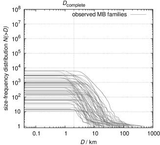
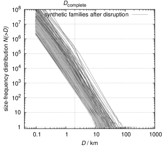
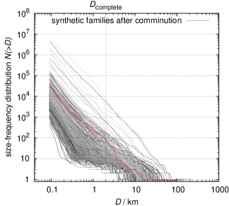
Figure 11: Left panel: the size-frequency distributions of the observed asteroid families. Middle panel: SFDs of 378 distinct synthetic families created during one of the collisional simulations of the MB and comets. Initially, all synthetic SFDs are very steep, in agreement with SPH simulations (Durda et al. 2007). We plot only the SFDs that fulfil the following criteria: $D_{\rm PB}\geq 50$ km, $D_{\rm LF}\geq 10$ km, ${\rm LR}/{\rm PB}<0.5$ (i.e. catastrophic disruptions). Right panel: the evolved SFDs after comminution. Only a minority of families are observable now, since the number of remaining members larger than the observational limit $D_{\rm limit}\simeq 2$ km is often much smaller than $100$. The SFD that we use for the simulation in Section 10 is denoted by red.

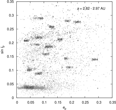
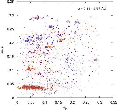
Figure 12: The “pristine zone” of the main belt ($a_{\rm p}=2.825\hbox{ to }2.955\,{\rm AU}$) displayed on the proper eccentricity $e_{\rm p}$ vs proper inclination $\sin I_{\rm p}$ plot. Left panel: the sizes of symbols correspond to the sizes of asteroids, the families are denoted by designations. Right panel: a subset of bodies for which SDSS data are available; the colours of symbols correspond to the SDSS colour indices $a^{*}$ and $i-z$ (Parker et al. 2008).

10 “Pristine zone” between the 5:2 and 7:3 resonances

We now focus on the zone between the 5:2 and 7:3 mean-motion resonances, with $a_{\rm p}=2.825\hbox{ to }2.955\,{\rm AU}$, which is not as populated as the surrounding regions of the main belt (see Figure 1). This is a unique situation, because both bounding resonances are strong enough to prevent any asteroids from outside to enter this zone owing the Yarkovsky semimajor axis drift. Any family formation event in the surroundings has only a minor influence on this narrow region. It thus can be called “pristine zone” because it may resemble the belt prior to creation of big asteroid families.

We identified nine previously unknown small families that are visible on the $(e_{\rm p},\sin I_{\rm p})$ plot (see Figure 12). They are confirmed by the SDSS colours and WISE albedos, too. Nevertheless, there is only one big and old family in this zone ($D_{\rm PB}\geq 100\,{\rm km}$), i.e. Koronis.

That at most one LHB family (Koronis) is observed in the “pristine zone” can give us a simple probabilistic estimate for the maximum number of disruptions during the LHB. We take the 192 existing main-belt bodies which have $D\geq 100\,{\rm km}$ and select randomly 100 of them that will break apart. We repeat this selection 1000 times and always count the number of families in the pristine zone. The resulting histogram is shown in Figure 13. As we can see, there is very low ($<$0.001) probability that the number of families in the pristine zone is zero or one. On average we get eight families there, i.e. about half of the 16 asteroids with $D\geq 100\,{\rm km}$ present in this zone. It seems that either the number of disruptions should be substantially lower than 100 or we expect to find at least some “remnants” of the LHB families here.

It is interesting that the SFD of an old comminutioned family is very flat in the range $D=1\hbox{ to }10\,{\rm km}$ (see Figure 11) — similar to those of some of the “less certain” observed families! We may speculate that the families like (918) Itha, (5567) Durisen, (12573) 1999 NJ₅₃, or (15454) 1998 YB₃ (all from the pristine zone) are actually remnants of larger and older families, even though they are denoted as young. It may be that the age estimate based on the $(a_{\rm p},H)$ analysis is incorrect since small bodies were destroyed by comminution and spread by the Yarkovsky effect too far away from the largest remnant, so they can no longer be identified with the family.

Finally, we have to ask an important question: what does an old/comminutioned family with $D_{\rm PB}\simeq 100\,{\rm km}$ look like in proper-element space? To this aim, we created a synthetic family in the “pristine zone”, and assumed the family has $N_{\rm members}\simeq 100$ larger than $D_{\rm limit}\simeq 2\,{\rm km}$ and that the SFD is already flat in the $D=1\hbox{ to }10\,{\rm km}$ range. We evolved the asteroids up to 4 Gyr due to the Yarkovsky effect and gravitational perturbations, using the N-body integrator as in Section 6. Most of the $D\simeq 2\,{\rm km}$ bodies were lost in the course of the dynamical evolution, of course. The resulting family is shown in Figure 14. We can also imagine that this family is placed in the pristine zone among other observed families, to get a feeling of whether it is easily observed or not (refer to Figure 12).

It is clear that such family is hardly observable even in the almost empty zone of the main belt! Our conclusion is that the comminution (as given by the Boulder code) can explain the paucity of $D_{\rm PB}\simeq 100\,{\rm km}$ LHB families, since we can hardly distinguish old families from the background.

Figure 13: The histogram for the expected number of LHB families located in the “pristine zone” of the main belt.

Figure 14: The proper eccentricity vs proper inclination of one synthetic old/comminutioned family evolved dynamically over 4 Gyr. Only a few family members ($N\simeq 10^{1}$) remained from the original number of $N(D\!\geq\!2\,{\rm km})\simeq 10^{2}$. The scales are the same as in Figure 12, so we can compare it easily to the “pristine zone”.

11 Conclusions

In this paper we investigated the cometary bombardment of the asteroid belt at the time of the LHB, in the framework of the Nice model. There is much evidence of a high cometary flux through the giant planet region, but no strong evidence of a cometary bombardment on the Moon. This suggests that many comets broke up on their way to the inner solar system. By investigating the collisional evolution of the asteroid belt and comparing the results to the collection of actual collisional families, our aim was to constrain whether the asteroid belt experienced an intense cometary bombardment at the time of the LHB and, if possible, constrain the intensity of this bombardment.

Observations suggest that the number of collisional families is a very shallow function of parent-body size (that we call in this paper the “production function”). We show that the collisional activity of the asteroid belt as a closed system, i.e. without any external cometary bombardment, in general does not produce such a shallow production function. Moreover, the number of families with parent bodies larger than 200 km in diameter is in general too small compared to the observations. However, there is a lot of stochasticity in the collisional evolution of the asteroid belt, and about 5 % of our simulations actually fit the observational constraints (shallowness of the production function and number of large families) quite well. Thus, in principle, there is no need for a bombardment due to external agents (i.e. the comets) to explain the asteroid family collection, provided that the real collisional evolution of the main belt was a “lucky” one and not the “average” one.

If one accounts for the bombardment provided by the comets crossing the main belt at the LHB time, predicted by the Nice model, one can easily justify the number of observed families with parent bodies larger than 200 km. However, the resulting production function is steep, and the number of families produced by parent bodies of 100 km is almost an order of magnitude too large.

We have investigated several processes that may decimate the number of families identifiable today with 100 km parent bodies, without considerably affecting the survival of families formed from larger parent bodies. Of all these processes, the collisional comminution of the families and their dispersal by the Yarkovsky effect are the most effective ones. Provided that the physical disruption of comets due to activity reduced the effective cometary flux through the belt by a factor of $\approx 5$, the resulting distribution of families (and consequently the Nice model) is consistent with observations.

To better quantify the effects of various cometary-disruption laws, we computed the numbers of asteroid families for different critical perihelion distances $q_{\rm crit}$ and for different disruption probabilities $p_{\rm crit}$ of comets during a given time step ($\Delta t=500\,{\rm yr}$ in our case). The results are summarised in Figure 15. Provided that comets are disrupted frequently enough, namely the critical perihelion distance has to be at least $q_{\rm crit}\gtrsim 1\,{\rm AU}$, while the probability of disruption is $p_{\rm crit}=1$, the number of $D_{\rm PB}\geq 100\,$km families drops by the aforementioned factor of $\approx 5$. Alternatively, $q_{\rm crit}$ may be larger, but then comets have to survive multiple perihelion passages (i.e. $p_{\rm crit}$ have to be lower than 1). It would be very useful to test these conditions by independent models of the evolution and physical disruptions of comets. Such additional constraints on cometary-disruption laws would then enable study of the original size-frequency distribution of the cometary disk in more detail.

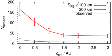
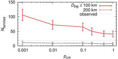
Figure 15: The numbers of collisional families for different critical perihelion distances $q_{\rm crit}$ at which comets break up and disruption probabilities $p_{\rm crit}$ during one time step ($\Delta t=500\,{\rm yr}$). In the top panel, we vary $q_{\rm crit}$ while keeping $p_{\rm crit}=1$ constant. In the bottom panel, $q_{\rm crit}=1.5\,{\rm AU}$ is constant and we vary $p_{\rm crit}$. We always show the number of catastrophic disruptions with parent-body sizes $D_{\rm PB}\geq 100\,{\rm km}$ (red line) and 200 km (black line). The error bars indicate typical (1-$\sigma$) spreads of Boulder simulations with different random seeds. The observed numbers of corresponding families are indicated by thin dotted lines.

We can also think of two “alternative” explanations: i) physical lifetime of comets was strongly size-dependent so that smaller bodies break up easily compared to bigger ones; ii) high-velocity collisions between hard targets (asteroids) and very weak projectiles (comets) may result in different outcomes than in low-velocity regimes explored so far. Our work thus may also serve as a motivation for further SPH simulations.

We finally emphasize that any collisional/dynamical models of the main asteroid belt would benefit from the following advances:

• determination of reliable masses of asteroids of various classes. This may be at least partly achieved by the Gaia mission in the near future. Using up-to-date sizes and shape models (volumes) of asteroids one can then derive their densities, which are directly related to ages of asteroid families.

• Development of methods for identifying asteroid families and possibly targeted observations of larger asteroids addressing their membership, which is sometimes critical for constructing size-frequency distributions and for estimating parent-body sizes.

• An extension of the SHP simulations for both smaller and larger targets, to assure that the scaling we use now is valid. Studies and laboratory measurements of equations of states for different materials (e.g. cometary-like, porous) are closely related to this issue.

The topics outlined above seem to be the most urgent developments to be pursued in the future.

References

- (1) Bendjoya, P., Cellino, A., Froeschlé, C., Zappalà, V. 1993, A&A, 272, 651
- (2) Benz, W., & Asphaug, E. 1999, Icarus, 142, 5
- (3) Bogard, D.D. 1995, Meteoritics, 30, 244
- (4) Bogard, D.D. 2011, Chemie der Erde – Geochemistry, 71, 207
- (5) Bottke, W.F., Vokrouhlický, D., Brož, M., Nesvorný, D., & Morbidelli, A. 2001, Science, 294, 1693
- (6) Bottke, W.F., Durda, D.D., Nesvorný, D., et al. 2005, Icarus, 175, 111
- (7) Bottke, W.F., Levison, H.F., Nesvorný, D., & Dones, L. 2007, Icarus, 190, 203
- (8) Bottke, W.F., Vokrouhlický, D., & Nesvorný, D. 2007, Nature, 449, 48
- (9) Bottke, W.F., Nesvorný, D., Vokrouhlický, D., & Morbidelli, A. 2010, AJ, 139, 994
- (10) Bottke, W.F., Vokrouhlický D., Minton, D., et al. 2012, Nature, 485, 78
- (11) Brož, M. 2006, PhD thesis, Charles Univ.
- (12) Brož, M., Vokrouhlický, D., Morbidelli, A., Nesvorný. D., & Bottke, W.F. 2011, MNRAS, 414, 2716
- (13) Carruba, V. 2009, MNRAS, 398, 1512
- (14) Carruba, V. 2010, MNRAS, 408, 580
- (15) Carry, B. 2012, arXiv: 1203.4336v1
- (16) Cellino, A., Zappalà, V., di Martino, M., Farinella, P., Paolicchi, P. 1987, Icarus, 70, 546
- (17) Chapman, C.R., Cohen, B.A., Grinspoon, D.H. 2007, Icarus, 189, 233
- (18) Charnoz, S., Morbidelli, A., Dones, L., & Salmon, J. 2009, Icarus, 199, 413
- (19) Cohen, B.A., Swindle, T.D., & Kring, D.A. 2000, Science, 290, 1754
- (20) Dahlgren, M. 1998, A&A, 336, 1056
- (21) Durda, D.D., Bottke, W.F., Nesvorný, D., et al. 2007, 186, 498
- (22) Foglia, S., & Masi, G., 2004, Minor Planet Bull., 31, 100
- (23) Gil-Hutton, R. 2006, Icarus, 183, 83
- (24) Gomes, R., Levison, H.F., Tsiganis, K., & Morbidelli, A. 2005, Nature, 435, 466
- (25) Hartmann, W.K., Ryder, G., Dones, L., & Grinspoon, D. 2000, in Origin of the Earth and Moon, ed. R.M. Canup, K. Righter, Tucson: University of Arizona Press, p. 493
- (26) Hartmann, W.K., Quantin, C., & Mangold, N. 2007, Icarus, 186, 11
- (27) Keil, K. 2002, in Asteroids III, ed. W.F. Bottke Jr., A. Cellino, P. Paolicchi, R.P. Binzel, Tucson: University of Arizona Press, p. 573
- (28) Kirchoff, M.R., & Schenk, P. 2010, Icarus, 206, 485
- (29) Knežević, Z., & Milani, A. 2003, A&A, 403, 1165
- (30) Koeberl, C. 2004, Geochimica et Cosmochimica Acta, 68, 931
- (31) Kring, D.A., & Cohen, B.A. 2002, J. Geophys. Res., 107, 41
- (32) Laskar, J., & Robutel, P. 2001, Celest. Mech. Dyn. Astron., 80, 39
- (33) Levison, H.F., & Duncan, M. 1994, Icarus, 108, 18
- (34) Levison, H.F., Bottke, W.F., Gounelle, M., et al. 2009, Nature, 460, 364
- (35) Margot, J.-L., & Rojo, P. 2007, BAAS, 39, 1608
- (36) Marzari, F., Farinella, P., & Davis, D.R. 1999, Icarus, 142, 63
- (37) Masiero, J.P., Mainzer A.K., Grav, T., et al. 2011, ApJ, 741, 68
- (38) Michel, P., Tanga, P., Benz, & W., Richardson, D.C. 2002, Icarus, 160, 10
- (39) Michel, P., Jutzi, M., Richardson, D.C., & Benz, W. 2011, Icarus, 211, 535
- (40) Minton, D.A., & Malhotra, R. 2009, Nature, 457, 1109
- (41) Minton, D.A., & Malhotra, R. 2010, Icarus, 207, 744
- (42) Morbidelli, A. 2010, Comptes Rendus Physique, 11, 651
- (43) Morbidelli, A., Tsiganis, K., Crida, A., Levison, H.F., & Gomes, R. 2007, AJ, 134, 1790
- (44) Morbidelli, A., Levison, H.F., Bottke, W.F., Dones, L., & Nesvorný, D. 2009, Icarus, 202, 310
- (45) Morbidelli, A., Brasser, R., Gomes, R., Levison, H.F., & Tsiganis, K. 2010, AJ, 140, 1391
- (46) Morbidelli, A., Marchi, S., & Bottke, W.F. 2012, LPI Cont. 1649, 53
- (47) Molnar, L.A., & Haegert, M.J. 2009, BAAS, 41, 2705
- (48) Nesvorný, D. 2010, EAR-A-VARGBDET-5-NESVORNYFAM-V1.0, NASA Planetary Data System
- (49) Nesvorný, D., & Vokrouhlický, D. 2006, AJ, 132, 1950
- (50) Nesvorný, D., Morbidelli, A., Vokrouhlický, D., Bottke, W.F., & Brož, M. 2002, Icarus, 157, 155
- (51) Nesvorný, D., Jedicke, R., Whiteley, R.J., & Ivezić, Ž. 2005, Icarus, 173, 132
- (52) Nesvorný, D., Vokrouhlický, D., & Morbidelli, A. 2007, AJ, 133, 1962
- (53) Nesvorný, D., Vokrouhlický, D., Morbidelli, A., & Bottke, W.F. 2009, Icarus, 200, 698
- (54) Neukum, G., Ivanov, B.A., & Hartmann, W.K. 2001, Space Sci. Rev., 96, 55
- (55) Norman, M.D., & Nemchin, A.A. 2012, LPI Cont., 1659, 1368
- (56) Novaković, B. 2010, MNRAS, 407, 1477
- (57) Novaković, B., Tsiganis, K., & Knežević, Z. 2010, Celest. Mech. Dyn. Astron., 107, 35
- (58) Novaković, B., Cellino, A., & Knežević, Z. 2011, Icarus, 216, 69
- (59) Parker, A., Ivezić, Ž., Jurić, M, et al. 2008, Icarus, 198, 138
- (60) Ryder, G., Koeberl, C., & Mojzsis, S.J. 2000, in Origin of the Earth and Moon, ed. R.M. Canup, K. Righter, Tucson: University of Arizona Press, p. 475
- (61) Sheppard, S.S, & Trujillo, C.A. 2010, ApJL, 723, L233
- (62) Strom, R.G., Malhotra, R., Ito, T., Yoshida, F., & Kring, D.A. 2005, Science, 309, 1847.
- (63) Swindle, T.D., Isachsen, C.E., Weirich, J.R., & Kring, D.A. 2009, Meteor. Planet. Sci., 44, 747
- (64) Tagle, R. 2005, LPI Cont., 36, 2008
- (65) Tanga, P., Cellino, A., Michel, P., Zappalà, V., Paolicchi, P., & Dell’Oro, A. 1999, Icarus, 141, 65
- (66) Tedesco, E.F., Noah, P.V., Noah, M., & Price, S.D. 2002, AJ, 123, 1056
- (67) Tera, F., Papanastassiou, D.A., & Wasserburg, G.J. 1974, Earth & Planet. Sci. Let., 22, 1
- (68) Tsiganis K., Gomes, R., Morbidelli, A., & Levison, H.F. 2005, Nature, 435, 459
- (69) Thomas, P.C., Binzel, R.P., Gaffey, M.J., et al. 1997, Science, 277, 1492
- (70) Vokrouhlický, D., & Nesvorný, D. 2011, AJ, 142, 26
- (71) Vokrouhlický, D., Brož, M., Bottke, W.F., Nesvorný, D., & Morbidelli, A. 2006, Icarus, 182, 118
- (72) Vokrouhlický, D., Nesvorný, D., & Levison, H.F. 2008, AJ, 136, 1463
- (73) Vokrouhlický, D., Nesvorný, D., Bottke, W.F., & Morbidelli, A. 2010, AJ, 139, 2148
- (74) Warner, B.D., Harris, A.W., Vokrouhlický, D., Nesvorný, D., & Bottke, W.F. 2009, Icarus, 204, 172
- (75) Weidenschilling, S.J. 2000, Space Sci. Rev., 92, 295
- (76) Zappalà, V., Bendjoya, Ph., Cellino, A., Farinella, P., & Froeschlé, C. 1995, Icarus, 116, 291