Optimistic limits of Kashaev invariants and complex volumes of hyperbolic links

Abstract

Yokota suggested an optimistic limit method of the Kashaev invariants of hyperbolic knots and showed it determines the complex volumes of the knots. His method is very effective and gives almost combinatorial method of calculating the complex volumes. However, to describe the triangulation of the knot complement, he restricted his method to knot diagrams with certain conditions. Although these restrictions are general enough for any hyperbolic knots, we have to select a good diagram of the knot to apply his theory.

In this article, we suggest more combinatorial way to calculate the complex volumes of hyperbolic links using the modified optimistic limit method. This new method works for any link diagrams, and it is more intuitive, easy to handle and has natural geometric meaning.

1 Introduction

Kashaev conjectured the following relation in [8] :

$$2\pi\lim_{N\rightarrow\infty}\frac{\log|\langle L\rangle_{N}|}{N}={\rm vol}(L),$$

where $L$ is a hyperbolic link, vol($L$) is the hyperbolic volume of $\mathbb{S}^{3}\backslash L$, and $\langle L\rangle_{N}$ is the $N$-th Kashaev invariant of $L$. After that, the generalized conjecture was proposed in [14] that

$$2\pi i\lim_{N\rightarrow\infty}\frac{\log\langle L\rangle_{N}}{N}\equiv i({\rm vol}(L)+i\,{\rm cs}(L))~{}~{}({\rm mod}~{}\pi^{2}),$$

where cs($L$) is the Chern-Simons invariant of $\mathbb{S}^{3}\backslash L$ defined modulo $\pi^{2}$ in [11]. These are now called Kashaev volume conjectures and ${\rm vol}(L)+i\,{\rm cs}(L)$ is called the complex volume of $L$.

When Kashaev suggested the conjecture in [8], he calculated a certain value using an analytic function induced from the Kashaev invariant and showed numerically that the value coincides with the volume of the link for a few cases, where the function was the same one called the potential function in [15]. After that, the value was named the optimistic limit of the Kashaev invariant and denoted by $2\pi i\,\underset{N\rightarrow\infty}{\text{\rm o-lim}}\frac{\log\langle L\rangle_{N}}{N}$ in [12]. (See Section 1.1 of [5] for the exact meaning of the optimistic limit.)

The potential function is closely related to the quantum dilogarithm function of Faddeev as in [8], especially, it can be considered as a classical limit of the partition function defined in [7], where the partition function is defined by assigning the quantum dilogarithms to each hyperbolic ideal tetrahedra and integrating the product of them. Quantum dilogarithm satisfies the 3–2 Pachner move, so the partition function is expected to be independent of the chosen triangulation. Similar ideas were used in [2] and [1] to define quantum (hyperbolic) field theories and certain invariants of knots incompact oriented 3-manifolds using partition functions, which suggests the potential functions can be used, not only in the optimistic limits, but also in many other situations.

Regarding the optimistic limit, Yokota proved

$$2\pi i\,\underset{N\rightarrow\infty}{\text{\rm o-lim}}\frac{\log\langle K\rangle_{N}}{N}\equiv i({\rm vol}(K)+i\,{\rm cs}(K))~{}~{}({\rm mod}~{}\pi^{2}),$$

for hyperbolic knots $K$ in [19] by introducing natural geometry corresponding to the optimistic limit. Elaborating on the geometry, he defined a triangulation of $\mathbb{S}^{3}\backslash(K\cup\{\text{two points}\})$ and transformed it into the triangulation of $\mathbb{S}^{3}\backslash K$ by collapsing certain tetrahedra. He defined the potential function reflecting this collapsing process and proved the derivation of this function gives the hyperbolicity equations, i.e. Thurston’s gluing equations and the completeness conditions of the triangulation. (See Section 3 for the definitions.) His method is very effective and gives almost combinatorial method of calculating the complex volumes of hyperbolic knots. (See [3] for a brief survey.)

However, understanding Yokota’s method in [19] is not easy for several reasons. We think a major difficulty lies on the collapsing process of the triangulation. To make the collapsing works well, he deformed the knot diagram into certain (1,1)-tangle diagram satisfying several non-trivial conditions and restricted his method only to knots. Furthermore, the collapsing process twists the natural triangulation to a complicate one. To overcome these difficulties, we will develop new version of Yokota theory without collapsing process here. Our method does not need to deform the diagram because it is applicable to any link diagrams without restriction.

In Section 2 of this article, we define the natural potential function $V(z_{1},\ldots,z_{n})$ of a hyperbolic link $L$ combinatorially from the link diagram. Then we will consider the following set of equations

$$\mathcal{H}:=\left\{\left.\exp(z_{k}\frac{\partial V}{\partial z_{k}})=1\right|k=1,\ldots,n\right\}.$$ (1)

In Section 3, we introduce an ideal triangulation of $\mathbb{S}^{3}\backslash(L\cup\{\text{two points}\})$, and name it octahedral triangulation. It was the same one considered in [19] before the collapsing, and it also appeared in [17] as a natural triangulation of the link complement inside $\mathbb{S}^{2}\times[0,1]$. On the other hand, Luo considered ideal triangulations of closed 3-manifolds by removing vertices in [9] and considered their hyperbolicity equations. Later, Luo, Tillmann and many others considered ideal triangulations of any 3-manifolds by removing non-ideal vertices and found several properties of their hyperbolicity equations. (See [16] for example.) We consider the hyperbolicity equations of the octahedral triangulation in this sense. Note that this ideal triangulation of $\mathbb{S}^{3}\backslash(L\cup\{\text{two points}\})$ can be obtained by removing two non-ideal points from the triangulation of $\mathbb{S}^{3}\backslash L$, as in [16].

One of the most important properties of the potential function $V$ is the following proposition.

Proposition 1.1.

For a hyperbolic link $L$ with a fixed diagram, consider the potential function $V(z_{1},\ldots,z_{n})$ defined in Section 2. Then the set $\mathcal{H}$ defined in (1) becomes the hyperbolicity equations of the octahedral triangulation of $\mathbb{S}^{3}\backslash(L\cup\{\text{two points}\})$.

The exact construction of the triangulation and the proof will be in Section 3. We remark that this proposition also holds for the potential functions of the collapsed cases in [19] and [5], but the proof of this article is more natural and far easier than the previous ones. This is because the collapsing process distorts the natural geometry of the triangulation, so one has to keep track of the changes carefully.

Let $\mathcal{S}=\{(z_{1},\ldots,z_{n})\}$ be the set of solutions of $\mathcal{H}$ in $\mathbb{C}^{n}$. In this article, we always assume $\mathcal{S}\neq\emptyset$. Then, by Theorem 1 of [16], all edges in the octahedral triangulation are essential. (Essential edge roughly means it is not null-homotopic. See [16] for the exact definition.) Therefore, using Yoshida’s construction in Section 4.5 of [10], for a solution $\mathbb{z}\in\mathcal{S}$, we can obtain the boundary-parabolic representation

$$\rho_{\mathbb{z}}:\pi_{1}(\mathbb{S}^{3}\backslash L)\longrightarrow{\rm PSL}(2,\mathbb{C}).$$ (2)

Note that the volume ${\rm vol}(\rho_{\mathbb{z}})$ and the Chern-Simons invariant ${\rm cs}(\rho_{\mathbb{z}})$ of $\rho_{\mathbb{z}}$ were defined in [20]. We call ${\rm vol}(\rho_{\mathbb{z}})+i\,{\rm cs}(\rho_{\mathbb{z}})$ the complex volume of $\rho_{\mathbb{z}}$.

For the solution set $\mathcal{S}$, let $\mathcal{S}_{j}$ be a path component of $\mathcal{S}$ satisfying $\mathcal{S}=\cup_{j\in J}\mathcal{S}_{j}$ for some index set $J$. We assume $0\in J$ for notational convenience. To obtain well-defined values of the potential function $V(z_{1},\ldots,z_{n})$ (see Lemma 2.1), we slightly modify it to

$$V_{0}(z_{1},\ldots,z_{n}):=V(z_{1},\ldots,z_{n})-\sum_{k=1}^{n}\left(z_{k}\frac{\partial V}{\partial z_{k}}\right)\log z_{k}.$$ (3)

Then the main result of this article is as follows:

Theorem 1.2.

Let $L$ be a hyperbolic link with a fixed diagram and $V(z_{1},\ldots,z_{n})$ be the potential function of the diagram. Assume the solution set $\mathcal{S}=\cup_{j\in J}\mathcal{S}_{j}$ is not empty. Then, for any ${\mathbb{z}}\in\mathcal{S}_{j}$, $V_{0}({\mathbb{z}})$ is constant (depends only on $j$) and

$$V_{0}(\mathbb{z})\equiv i\,({\rm vol}(\rho_{\mathbb{z}})+i\,{\rm cs}(\rho_{\mathbb{z}}))~{}~{}({\rm mod}~{}\pi^{2}),$$ (4)

where $\rho_{\mathbb{z}}$ is the boundary-parabolic representation obtained in (2). Furthermore, there exists a path component $\mathcal{S}_{0}$ of $\mathcal{S}$ satisfying

$$V_{0}(\mathbb{z_{\infty}})\equiv i\,({\rm vol}(L)+i\,{\rm cs}(L))~{}~{}({\rm mod}~{}\pi^{2}),$$ (5)

for all ${\mathbb{z}}_{\infty}\in\mathcal{S}_{0}$.

The proof will be given in Section 4. The main idea is to use Zickert’s formula of the extended Bloch group in [20], which was already appeared in [19]. However, our proof is simpler because we do not consider any collapsing. We call the value $V_{0}({\mathbb{z}})$ the optimistic limit of the Kashaev invariant and note that it depends on the choice of the diagram and the path component $\mathcal{S}_{j}$. Finally, in Section 5, we apply our results to the twist knots and calculate the complex volumes of representations.

Although we restricted $L$ to hyperbolic links, Proposition 1.1 and Theorem 1.2 still hold for non-hyperbolic links except for the existence of $S_{0}$ and (5). (The definitions of ${\rm vol}(\rho_{\mathbb{z}})$ and ${\rm cs}(\rho_{\mathbb{z}})$ are from [20].) That is because we do not use the hyperbolic structure of $L$ but the boundary-parabolic representation $\rho_{\mathbb{z}}$ in (2), which can be non-discrete or non-faithful.

Finally, we remark that the following relation

$$J_{L}(N;\exp\frac{2\pi i}{N})=\langle L\rangle_{N}$$

was proved in [13], where $J_{L}(N;x)$ is the $N$-th colored Jones polynomial of $L$ with a complex variable $x$. Therefore, it is very natural to consider the optimistic limit of the colored Jones polynomial, and it will be discussed in the first author’s another article [4].

2 Potential function $V(z_{1},\ldots,z_{n})$

Consider a hyperbolic link $L$ and its diagram $D$. For simplicity, we always assume $D$ does not have any kink by removing them as in Figure 1.

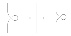
Figure 1: Removing kinks

We define sides of $D$ by the arcs connecting two adjacent crossing points. For example, the diagram of the figure-eight knot $4_{1}$ in Figure 2 has 8 sides.

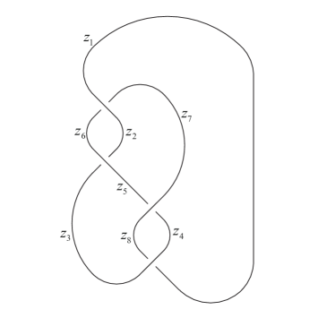
Figure 2: The figure-eight knot $4_{1}$

We assign complex variables $z_{1},\ldots,z_{n}$ to each side of the diagram $D$. Using the dilogarithm function ${\rm Li}_{2}(z)=-\int_{0}^{z}\frac{\log(1-t)}{t}dt$, we define the potential function of a crossing as in Figure 3.

Figure 3: Potential function of a crossing

Note that the potential function in Figure 3 comes from the formal substitution of the R-matrix of the Kashaev invariant in [18]. (See [5] for the meaning of the formal substitution.) In [3], we defined the potential function of the corner of a crossing from Figure 4. Following this definition, the potential function of a crossing is then the summation of potential functions of the four corners.

(a) Positive crossing

(b) Negative crossing

Figure 4: Potential function of a corner

The potential function $V(z_{1},\ldots,z_{n})$ of the diagram $D$ is defined by the summation of all potential functions of the crossings. For example, the potential function of the figure-eight knot $4_{1}$ in Figure 2 is

$$V(z_{1},\ldots,z_{8})=\left\{{\rm Li}_{2}(\frac{z_{6}}{z_{1}})-{\rm Li}_{2}(\frac{z_{6}}{z_{2}})+{\rm Li}_{2}(\frac{z_{7}}{z_{2}})-{\rm Li}_{2}(\frac{z_{7}}{z_{1}})\right\}$$

$$+\left\{{\rm Li}_{2}(\frac{z_{3}}{z_{6}})-{\rm Li}_{2}(\frac{z_{3}}{z_{5}})+{\rm Li}_{2}(\frac{z_{2}}{z_{5}})-{\rm Li}_{2}(\frac{z_{2}}{z_{6}})\right\}$$

$$+\left\{{\rm Li}_{2}(\frac{z_{4}}{z_{8}})-{\rm Li}_{2}(\frac{z_{4}}{z_{7}})+{\rm Li}_{2}(\frac{z_{5}}{z_{7}})-{\rm Li}_{2}(\frac{z_{5}}{z_{8}})\right\}$$

$$+\left\{{\rm Li}_{2}(\frac{z_{1}}{z_{3}})-{\rm Li}_{2}(\frac{z_{1}}{z_{4}})+{\rm Li}_{2}(\frac{z_{8}}{z_{4}})-{\rm Li}_{2}(\frac{z_{8}}{z_{3}})\right\}.$$

We define a modified potential function $V_{0}(z_{1},\ldots,z_{n})$ as given in (3). Note that $V_{0}$ is analytic since the dilogarithm function ${\rm Li}_{2}(z)$ is analytic and the term $z_{k}\frac{\partial V}{\partial z_{k}}$ consists of logarithms. This property will be used implicitly in Lemma 2.2 below.

Recall that $\mathcal{H}$ was defined in (1). Also recall that we are considering the solutions ${\mathbb{z}}=(z_{1},\ldots,z_{n})\in\mathbb{C}^{n}$ of $\mathcal{H}$ with the property that if the potential function is expressed by $V(z_{1},\ldots,z_{n})=\sum\pm{\rm Li}_{2}(\frac{z_{a}}{z_{b}})$, then variables inside the dilogarithms satisfy $\frac{z_{a}}{z_{b}}\notin\{0,1,\infty\}$. This choice is reasonable because, if $\frac{z_{a}}{z_{b}}\in\{0,1,\infty\}$ for some solution, then at least one of the terms $\frac{\partial V}{\partial z_{a}}$ and $\frac{\partial V}{\partial z_{b}}$ of $V_{0}(z_{1},\ldots,z_{n})$ is not well-defined at that solution.

In this article, we always assume the solution set $\mathcal{S}\subset\mathbb{C}^{n}$ of $\mathcal{H}$ is nonempty. We cannot guarantee $\mathcal{S}\neq\emptyset$ for any link diagram. For example, the link diagrams containing Figure 5 always satisfy $\mathcal{S}=\emptyset$ because $\exp(z_{4}\frac{\partial V}{\partial z_{4}})=1$ implies $z_{1}=z_{3}$. However, we can easily remove this problem by reducing the redundant crossings in this case. We expect that if $\mathcal{S}=\emptyset$ for a given link diagram, changing the diagram properly makes $\mathcal{S}\neq\emptyset$.

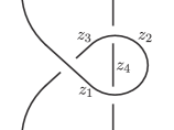
Figure 5: Diagram with $\mathcal{S}=\emptyset$

Note that the functions ${\rm Li}_{2}(z)$ and $\log z$ are multi-valued functions. Therefore, to obtain well-defined values, we have to select proper branch of the logarithm by choosing $\arg z$ and $\arg(1-z)$. The following lemma shows why we consider the potential function $V_{0}$ instead of $V$.

Lemma 2.1.

Let $\mathbb{z}=(z_{1},\ldots,z_{n})\in\mathcal{S}$. For the potential function $V(z_{1},\ldots,z_{n})$, the value of $V_{0}(\mathbb{z})$ is invariant under a choice of branch of the logarithm modulo $4\pi^{2}$.

Proof.

Let ${\rm Li}_{2}^{*}(z)$ and $\log^{*}z$ be the functions with different log-branch corresponding to an analytic continuation of ${\rm Li}_{2}(z)$ and $\log z$ respectively. Also let $V(z_{1},\ldots,z_{n})=\sum\pm{\rm Li}_{2}(\frac{z_{l}}{z_{m}})$. Then

$${\rm Li}_{2}^{*}(\frac{z_{l}}{z_{m}})\equiv{\rm Li}_{2}(\frac{z_{l}}{z_{m}})+2a\pi i\log\frac{z_{l}}{z_{m}}~{}~{}({\rm mod}~{}4\pi^{2})$$

for a certain integer $a$,

$$\log^{*}z_{l}\equiv\log z_{l},~{}\log^{*}z_{m}\equiv\log z_{m},~{}\log^{*}\frac{z_{l}}{z_{m}}\equiv\log\frac{z_{l}}{z_{m}}~{}~{}({\rm mod}~{}2\pi i),$$

and, because of $\mathbb{z}=(z_{1},\ldots,z_{n})\in\mathcal{S}$, we have

$$z_{l}\frac{\partial({\sum\pm}{\rm Li}_{2}(\frac{z_{l}}{z_{m}}))}{\partial z_{l}}\equiv z_{m}\frac{\partial({\sum\pm}{\rm Li}_{2}(\frac{z_{l}}{z_{m}}))}{\partial z_{m}}\equiv 0~{}~{}({\rm mod}~{}2\pi i).$$

Therefore,

$${\sum\pm}\left\{{\rm Li}_{2}^{*}(\frac{z_{l}}{z_{m}})-\left(z_{l}\frac{\partial{\rm Li}_{2}^{*}({z_{l}}/{z_{m}})}{\partial z_{l}}\right)\log^{*}z_{l}-\left(z_{m}\frac{\partial{\rm Li}_{2}^{*}({z_{l}}/{z_{m}})}{\partial z_{m}}\right)\log^{*}z_{m}\right\}$$

$$\equiv {\sum\pm}\left\{{\rm Li}_{2}(\frac{z_{l}}{z_{m}})+2a\pi i\log\frac{z_{l}}{z_{m}}-\left(z_{l}\frac{\partial{\rm Li}_{2}({z_{l}}/{z_{m}})}{\partial z_{l}}\right)\log^{*}z_{l}-2a\pi i\log^{*}z_{l}\right.$$

$$\left.-\left(z_{m}\frac{\partial{\rm Li}_{2}({z_{l}}/{z_{m}})}{\partial z_{m}}\right)\log^{*}z_{m}+2a\pi i\log^{*}z_{m}\right\}$$

$$\equiv {\sum\pm}\left\{{\rm Li}_{2}(\frac{z_{l}}{z_{m}})+2a\pi i\log\frac{z_{l}}{z_{m}}-\left(z_{l}\frac{\partial{\rm Li}_{2}({z_{l}}/{z_{m}})}{\partial z_{l}}\right)\log z_{l}-2a\pi i\log z_{l}\right.$$

$$\left.-\left(z_{m}\frac{\partial{\rm Li}_{2}({z_{l}}/{z_{m}})}{\partial z_{m}}\right)\log z_{m}+2a\pi i\log z_{m}\right\}$$

$$\equiv {\sum\pm}\left\{{\rm Li}_{2}(\frac{z_{l}}{z_{m}})-\left(z_{l}\frac{\partial{\rm Li}_{2}({z_{l}}/{z_{m}})}{\partial z_{l}}\right)\log z_{l}-\left(z_{m}\frac{\partial{\rm Li}_{2}({z_{l}}/{z_{m}})}{\partial z_{m}}\right)\log z_{m}\right\}~{}~{}({\rm mod}~{}4\pi^{2}).$$

The potential function $V_{0}$ is the summation of the above terms, so the proof follows.

∎

Lemma 2.2.

Let $\mathcal{S}=\cup_{j\in J}\mathcal{S}_{j}\subset\mathbb{C}^{n}$ be the solution set of $\mathcal{H}$ with $\mathcal{S}_{j}$ being a path component. Assume $\mathcal{S}\neq\emptyset$. Then, for any ${\mathbb{z}}=(z_{1},\ldots,z_{n})\in\mathcal{S}_{j}$,

$$V_{0}({\mathbb{z}})\equiv C_{j}~{}~{}({\rm mod}~{}4\pi^{2}),$$

where $C_{j}$ is a complex constant depending only on $j\in J$.

Proof.

Note that $z_{k}\frac{\partial V}{\partial z_{k}}$ is continuous on $\mathcal{S}_{j}$ and $\exp(z_{k}\frac{\partial V}{\partial z_{k}})=1$ for any ${\mathbb{z}}\in\mathcal{S}$. Therefore,

$$z_{k}\frac{\partial V}{\partial z_{k}}=r_{j,k}\pi i,$$ (6)

on $\mathcal{S}_{j}$ for an integer constant $r_{j,k}$ depending on $j$ and $k$. (The integer $r_{j,k}$ can be changed when $\mathbb{z}$ passes through the branch cut of the logarithm. In this case, we change the branch cut so that $r_{j,k}$ is locally constant. The global invariance of $V_{0}$ is obtained by the local invariance discussed below and Lemma 2.1.)

For any path

$$\mathbf{a}(t)=(\alpha_{1}(t),\ldots,\alpha_{n}(t)):[0,1]\longrightarrow\mathcal{S}_{j},$$

using (6) and the Chain rule, we have

$$\frac{dV_{0}}{dt}(\mathbf{a}(t)) = \frac{dV}{dt}(\mathbf{a}(t))-\frac{d}{dt}\left(\sum_{k=1}^{n}r_{j,k}\pi i\log\alpha_{k}(t)\right)$$

$$= \sum_{k=1}^{n}\frac{\partial V}{\partial z_{k}}(\mathbf{a}(t))\alpha_{k}^{\prime}(t)-\sum_{k=1}^{n}r_{j,k}\pi i\frac{\alpha_{k}^{\prime}(t)}{\alpha_{k}(t)}$$

$$= \sum_{k=1}^{n}\frac{r_{j,k}\pi i}{\alpha_{k}(t)}\alpha_{k}^{\prime}(t)-\sum_{k=1}^{n}r_{j,k}\pi i\frac{\alpha_{k}^{\prime}(t)}{\alpha_{k}(t)}=0.$$

This implies $V_{0}$ is constant on $\mathcal{S}_{j}$.

∎

Although we are considering the solution set $\mathcal{S}$ in $\mathbb{C}^{n}$, it is more natural to consider $\mathcal{S}$ as a subset of the complex projective space $\mathbb{CP}^{n-1}$. This fact is not used in this article, but we show the following lemma for reference.

Corollary 2.3.

If ${\mathbb{z}}=(z_{1},\ldots,z_{n})\in\mathcal{S}_{j}$, then $\lambda{\mathbb{z}}:=(\lambda z_{1},\ldots,\lambda z_{n})\in\mathcal{S}_{j}$ for any nonzero complex number $\lambda$. Furthermore,

$$V_{0}({\mathbb{z}})\equiv V_{0}(\lambda{\mathbb{z}})~{}~{}({\rm mod}~{}4\pi^{2}).$$

Proof.

The equations in $\mathcal{H}$ are products of the following terms

$$\exp\left(z_{l}\frac{\partial{\rm Li}_{2}(z_{l}/z_{m})}{\partial z_{l}}\right)=\left(1-\frac{z_{l}}{z_{m}}\right)^{-1}\text{ and }\exp\left(z_{m}\frac{\partial{\rm Li}_{2}(z_{l}/z_{m})}{\partial z_{m}}\right)=\left(1-\frac{z_{l}}{z_{m}}\right),$$

which are represented only with ratios of the variables. This proves the first statement.

The second statement comes from Lemma 2.2 by choosing a path from ${\mathbb{z}}$ to $\lambda{\mathbb{z}}$.

∎

3 Octahedral triangulation of $\mathbb{S}^{3}\backslash(L\cup\{\text{two points}\})$

In this section, we describe an ideal triangulation of $\mathbb{S}^{3}\backslash(L\cup\{\text{two points}\})$. We remark that this triangulation was already appeared in many different places because it naturally came from the link diagram. (For example, see Section 3 of [17].) It was also appeared in Section 2.1 of [5] and we named it (uncollapsed) Yokota triangulation.

To obtain the triangulation, we place an octahedron ${\rm A}_{k}{\rm B}_{k}{\rm C}_{k}{\rm D}_{k}{\rm E}_{k}{\rm F}_{k}$ on each crossing $k$ as in Figure 6 and twist it by identifying edges ${\rm B}_{k}{\rm F}_{k}$ to ${\rm D}_{k}{\rm F}_{k}$ and ${\rm A}_{k}{\rm E}_{k}$ to ${\rm C}_{k}{\rm E}_{k}$ respectively. The edges ${\rm A}_{k}{\rm B}_{k}$, ${\rm B}_{k}{\rm C}_{k}$, ${\rm C}_{k}{\rm D}_{k}$ and ${\rm D}_{k}{\rm A}_{k}$ are called horizontal edges and we sometimes express these edges in the diagram as arcs around the crossing in the left hand side of Figure 6.

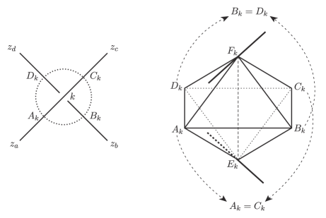
Figure 6: Octahedron on the crossing $k$

Then we glue faces of the octahedra following the sides of the diagram. Specifically, there are three gluing patterns as in Figure 7. In each cases (a), (b) and (c), we identify the faces $\triangle{\rm A}_{k}{\rm B}_{k}{\rm E}_{k}\cup\triangle{\rm C}_{k}{\rm B}_{k}{\rm E}_{k}$ to $\triangle{\rm C}_{k+1}{\rm D}_{k+1}{\rm F}_{k+1}\cup\triangle{\rm C}_{k+1}{\rm B}_{k+1}{\rm F}_{k+1}$, $\triangle{\rm B}_{k}{\rm C}_{k}{\rm F}_{k}\cup\triangle{\rm D}_{k}{\rm C}_{k}{\rm F}_{k}$ to $\triangle{\rm D}_{k+1}{\rm C}_{k+1}{\rm F}_{k+1}\cup\triangle{\rm B}_{k+1}{\rm C}_{k+1}{\rm F}_{k+1}$ and $\triangle{\rm A}_{k}{\rm B}_{k}{\rm E}_{k}\cup\triangle{\rm C}_{k}{\rm B}_{k}{\rm E}_{k}$ to $\triangle{\rm C}_{k+1}{\rm B}_{k+1}{\rm E}_{k+1}\cup\triangle{\rm A}_{k+1}{\rm B}_{k+1}{\rm E}_{k+1}$ respectively.

Figure 7: Three gluing patterns

Note that this gluing process identifies vertices $\{{\rm A}_{k},{\rm C}_{k}\}$ to one point, denoted by $-\infty$, and $\{{\rm B}_{k},{\rm D}_{k}\}$ to another point, denoted by $\infty$, and finally $\{{\rm E}_{k},{\rm F}_{k}\}$ to the other points, denoted by ${\rm P}_{j}$ where $j=1,\ldots,s$ and $s$ is the number of the components of the link $L$. The regular neighborhoods of $-\infty$ and $\infty$ are 3-balls and that of $\cup_{j=1}^{s}P_{j}$ is a tubular neighborhood of the link $L$. Therefore, if we remove the vertices ${\rm P}_{1},\ldots,{\rm P}_{s}$ from the gluing, then we obtain a triangulation of $\mathbb{S}^{3}\backslash L$, denoted by $\mathcal{T}$. On the other hand, if we remove all the vertices of the gluing, the result becomes an ideal triangulation of $\mathbb{S}^{3}\backslash(L\cup\{\pm\infty\})$. We call this ideal triangulation octahedral triangulation and denote it by $\mathcal{T}^{\prime}$.

Let $M=\mathbb{S}^{3}\backslash L$ and $M^{\prime}=\mathbb{S}^{3}\backslash(L\cup\{\pm\infty\})$. Then there exists a continuous deformation of the developing maps from $\widetilde{M}\longrightarrow\mathbb{H}^{3}$ to $\widetilde{M^{\prime}}\longrightarrow\mathbb{H}^{3}$, called Thurston’s spinning construction. Section 3 of [10] explains this construction for closed manifolds, but it can be applied to our triangulation $\mathcal{T}$ by fixing ideal points ${\rm P}_{1},\ldots,{\rm P}_{s}$ and sending points $\pm\infty$ to $\partial\overline{\mathbb{H}^{3}}=\mathbb{CP}^{1}$. Therefore, the parameter space of $\mathcal{T}^{\prime}$ in [10] determines the complex volume of $M$. (We will apply Zickert’s formula of [20] to $\mathcal{T}^{\prime}$ for calculating the complex volumes of $M$. See Section 4 for details.)

To describe the parameter space of the octahedral triangulation $\mathcal{T}^{\prime}$, we divide each ideal octahedron ${\rm A}_{k}{\rm B}_{k}{\rm C}_{k}{\rm D}_{k}{\rm E}_{k}{\rm F}_{k}$ into four ideal tetrahedra ${\rm A}_{k}{\rm B}_{k}{\rm E}_{k}{\rm F}_{k}$, ${\rm B}_{k}{\rm C}_{k}{\rm E}_{k}{\rm F}_{k}$, ${\rm C}_{k}{\rm D}_{k}{\rm E}_{k}{\rm F}_{k}$ and ${\rm D}_{k}{\rm A}_{k}{\rm E}_{k}{\rm F}_{k}$. When $z_{a}$, $z_{b}$, $z_{c}$ and $z_{d}$ are assigned to the sides around the octahedron as in Figure 8, we parametrize each tetrahedra by assigning shape parameters $\frac{z_{b}}{z_{a}}$, $\frac{z_{c}}{z_{b}}$, $\frac{z_{d}}{z_{c}}$ and $\frac{z_{a}}{z_{d}}$ to the horizontal edges ${\rm A}_{k}{\rm B}_{k}$, ${\rm B}_{k}{\rm C}_{k}$, ${\rm C}_{k}{\rm D}_{k}$ and ${\rm D}_{k}{\rm A}_{k}$ respectively.

Figure 8: Parametrizing tetrahedra

Note that if we assign a shape parameter $u\in\mathbb{C}\backslash\{0,1\}$ to an edge of an ideal tetrahedron, then the other edges are also parametrized by $u,u^{\prime}:=\frac{1}{1-u}$ and $u^{\prime\prime}:=1-\frac{1}{u}$ as in Figure 9.

Figure 9: Parametrization of an ideal tetrahedron with a parameter $u$

For a given ideal triangulation of $\mathbb{S}^{3}\backslash L$ or $\mathbb{S}^{3}\backslash(L\cup\{\pm\infty\})$, we require two conditions to obtain the complete hyperbolic structure; the product of shape parameters on an edge is one for all edges, and the holonomies of meridian and longitude act as translations on the cusp. The former are called Thurston’s gluing equations and the latter completeness conditions. Note that these conditions are expressed as equations of shape parameters. The whole set of these equations are called the hyperbolicity equations. The works of Luo, Tillmann and others in [10] and [16] use only Thurston’s gluing equations, but, in this article, we also require completeness conditions. Therefore, if $\mathbb{z}$ is a solution of the hyperbolicity equations, then the induced representation $\rho_{\mathbb{z}}:\pi_{1}(\mathbb{S}^{3}\backslash L)\longrightarrow{\rm PSL}(2,\mathbb{C})$ is boundary-parabolic.

The rest of this section is devoted to the proof of Proposition 1.1. Note that Proposition 1.1 was already appeared and proved in [19] in a slightly different way.

Proof of Proposition 1.1.

For each octahedron in Figure 6 of the octahedral triangulation, let $\mathcal{A}$ be the set of horizontal edges ${\rm A}_{k}{\rm B}_{k}$, ${\rm B}_{k}{\rm C}_{k}$, ${\rm C}_{k}{\rm D}_{k}$ and ${\rm D}_{k}{\rm A}_{k}$ of all crossings $k$. Let $\mathcal{B}$ be the set of edges ${\rm B}_{k}{\rm F}_{k}$, ${\rm D}_{k}{\rm F}_{k}$, ${\rm A}_{k}{\rm E}_{k}$, ${\rm C}_{k}{\rm E}_{k}$ of all crossings and other edges glued to them. Let $\mathcal{C}$ be the set of edges ${\rm E}_{k}{\rm F}_{k}$ of all crossings and let $\mathcal{D}$ be set of the other edges in the triangulation. Note that if the diagram $D$ is alternating, then $\mathcal{D}=\emptyset$.

The rule of assigning shape parameters to horizontal edges makes the edge conditions of $\mathcal{A}$ and $\mathcal{C}$ hold trivially.

Lemma 3.1.

The set of equations $\mathcal{H}$ consists of the completeness conditions along the meridian and Thurston’s gluing equations of the elements in $\mathcal{D}$.

Proof.

Consider the following three cases in Figure 10. We call the case (a) alternating gluing and the other cases (b) and (c) non-alternating gluings. Note that elements of $\mathcal{D}$ appear only in non-alternating gluings. (Specifically ${\rm C}_{k}{\rm F}_{k}={\rm C}_{k+1}{\rm F}_{k+1}\in\mathcal{D}$ in the case (b) and ${\rm B}_{k}{\rm E}_{k}={\rm B}_{k+1}{\rm E}_{k+1}\in\mathcal{D}$ in the case (c).)

Figure 10: Three cases of gluings

The variables $z_{a},z_{b},z_{c},z_{d}$ and $z_{l}$ are assigned to each sides in Figure 10. The potential function $V^{(a)}$ of the four corners in Figure 10(a) is defined by

$$V^{(a)}={\rm Li}_{2}\left(\frac{z_{l}}{z_{a}}\right)+{\rm Li}_{2}\left(\frac{z_{b}}{z_{l}}\right)-{\rm Li}_{2}\left(\frac{z_{c}}{z_{l}}\right)-{\rm Li}_{2}\left(\frac{z_{l}}{z_{d}}\right),$$

and it induces the following equation

$$\exp\left(z_{l}\frac{\partial V}{\partial z_{l}}\right) = \exp\left(z_{l}\frac{\partial V^{(a)}}{\partial z_{l}}\right)$$ (7)

$$= \left(1-\frac{z_{l}}{z_{a}}\right)^{-1}\left(1-\frac{z_{b}}{z_{l}}\right)\left(1-\frac{z_{c}}{z_{l}}\right)^{-1}\left(1-\frac{z_{l}}{z_{d}}\right)=1\in\mathcal{H}.$$

On the other hand, the cusp along the side $z_{l}$ in Figure 10(a) can be visualized by the annulus in Figure 11. In Figure 11, $a_{k}$, $b_{k}$, $c_{k}$, $b_{k+1}$, $c_{k+1}$, $d_{k+1}$ are the points of the cusp, which lie on the edges ${\rm A}_{k}{\rm E}_{k}$, ${\rm B}_{k}{\rm E}_{k}$, ${\rm C}_{k}{\rm E}_{k}$, ${\rm B}_{k+1}{\rm F}_{k+1}$, ${\rm C}_{k+1}{\rm F}_{k+1}$, ${\rm D}_{k+1}{\rm F}_{k+1}$ respectively, and $m$ is the meridian of the cusp.

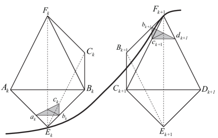
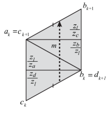
Figure 11: Cusp diagram of Figure 10(a)

The completeness condition along $m$ in Figure 11 becomes

$$\left\{\left(\frac{z_{d}}{z_{l}}\right)^{\prime\prime}\left(\frac{z_{l}}{z_{a}}\right)^{\prime}\right\}^{-1}\left(\frac{z_{b}}{z_{l}}\right)^{\prime}\left(\frac{z_{l}}{z_{c}}\right)^{\prime\prime}=\left(1-\frac{z_{l}}{z_{d}}\right)^{-1}\left(1-\frac{z_{l}}{z_{a}}\right)\left(1-\frac{z_{b}}{z_{l}}\right)^{-1}\left(1-\frac{z_{c}}{z_{l}}\right)=1,$$

which is equivalent to (7).

The potential function $V^{(b)}$ of the four corners in Figure 10(b) is defined by

$$V^{(b)}=-{\rm Li}_{2}\left(\frac{z_{a}}{z_{l}}\right)+{\rm Li}_{2}\left(\frac{z_{b}}{z_{l}}\right)-{\rm Li}_{2}\left(\frac{z_{c}}{z_{l}}\right)+{\rm Li}_{2}\left(\frac{z_{d}}{z_{l}}\right),$$

and it induces the following equation

$$\exp\left(z_{l}\frac{\partial V}{\partial z_{l}}\right) = \exp\left(z_{l}\frac{\partial V^{(b)}}{\partial z_{l}}\right)$$ (8)

$$= \left(1-\frac{z_{a}}{z_{l}}\right)^{-1}\left(1-\frac{z_{b}}{z_{l}}\right)\left(1-\frac{z_{c}}{z_{l}}\right)^{-1}\left(1-\frac{z_{d}}{z_{l}}\right)=1\in\mathcal{H}.$$

On the other hand, the cusp along the side $z_{l}$ in Figure 10(b) can be visualized by Figure 12. In Figure 12, $b_{k}$, $c_{k}$, $d_{k}$, $b_{k+1}$, $c_{k+1}$, $d_{k+1}$ are the points of the cusp, which lie on the edges ${\rm B}_{k}{\rm F}_{k}$, ${\rm C}_{k}{\rm F}_{k}$, ${\rm D}_{k}{\rm F}_{k}$, ${\rm B}_{k+1}{\rm F}_{k+1}$, ${\rm C}_{k+1}{\rm F}_{k+1}$, ${\rm D}_{k+1}{\rm F}_{k+1}$ respectively, and the edges $c_{k}d_{k}$ and $c_{k}b_{k}$ are identified to $c_{k+1}b_{k+1}$ and $c_{k+1}d_{k+1}$ respectively.

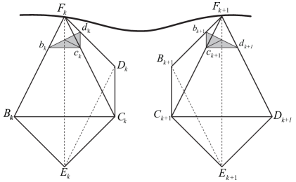
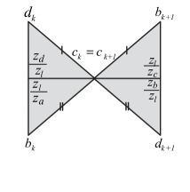
Figure 12: Cusp diagram of Figure 10(b)

Thurston’s gluing equation of the edge ${\rm C}_{k}{\rm F}_{k}={\rm C}_{k+1}{\rm F}_{k+1}\in\mathcal{D}$ (around $c_{k}=c_{k+1}$) in Figure 12 becomes

$$\left(\frac{z_{l}}{z_{a}}\right)^{\prime\prime}\left(\frac{z_{b}}{z_{l}}\right)^{\prime}\left(\frac{z_{l}}{z_{c}}\right)^{\prime\prime}\left(\frac{z_{d}}{z_{l}}\right)^{\prime}=\left(1-\frac{z_{a}}{z_{l}}\right)\left(1-\frac{z_{b}}{z_{l}}\right)^{-1}\left(1-\frac{z_{c}}{z_{l}}\right)\left(1-\frac{z_{d}}{z_{l}}\right)^{-1}=1,$$

which is equivalent to (8).

The potential function $V^{(c)}$ of the four corners in Figure 10(c) is defined by

$$V^{(c)}={\rm Li}_{2}\left(\frac{z_{l}}{z_{a}}\right)-{\rm Li}_{2}\left(\frac{z_{l}}{z_{b}}\right)+{\rm Li}_{2}\left(\frac{z_{l}}{z_{c}}\right)-{\rm Li}_{2}\left(\frac{z_{l}}{z_{d}}\right),$$

and it induces the following equation

$$\exp\left(z_{l}\frac{\partial V}{\partial z_{l}}\right) = \exp\left(z_{l}\frac{\partial V^{(c)}}{\partial z_{l}}\right)$$ (9)

$$= \left(1-\frac{z_{l}}{z_{a}}\right)^{-1}\left(1-\frac{z_{l}}{z_{b}}\right)\left(1-\frac{z_{l}}{z_{c}}\right)^{-1}\left(1-\frac{z_{l}}{z_{d}}\right)=1\in\mathcal{H}.$$

On the other hand, the cusp along the side $z_{l}$ in Figure 10(c) can be visualized by Figure 13. In Figure 13, $a_{k}$, $b_{k}$, $c_{k}$, $a_{k+1}$, $b_{k+1}$, $c_{k+1}$ are the points of the cusp, which lie on the edges ${\rm A}_{k}{\rm E}_{k}$, ${\rm B}_{k}{\rm E}_{k}$, ${\rm C}_{k}{\rm E}_{k}$, ${\rm A}_{k+1}{\rm E}_{k+1}$, ${\rm B}_{k+1}{\rm E}_{k+1}$, ${\rm C}_{k+1}{\rm E}_{k+1}$ respectively, and the edges $b_{k}a_{k}$ and $b_{k}c_{k}$ are identified to $b_{k+1}c_{k+1}$ and $b_{k+1}a_{k+1}$ respectively.

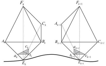
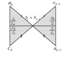
Figure 13: Cusp diagram of Figure 10(c)

Thurston’s gluing equation of the edge ${\rm B}_{k}{\rm E}_{k}={\rm B}_{k+1}{\rm E}_{k+1}\in\mathcal{D}$ (around $b_{k}=b_{k+1}$) in Figure 13 becomes

$$\left(\frac{z_{l}}{z_{a}}\right)^{\prime}\left(\frac{z_{b}}{z_{l}}\right)^{\prime\prime}\left(\frac{z_{l}}{z_{c}}\right)^{\prime}\left(\frac{z_{d}}{z_{l}}\right)^{\prime\prime}=\left(1-\frac{z_{l}}{z_{a}}\right)^{-1}\left(1-\frac{z_{l}}{z_{b}}\right)\left(1-\frac{z_{l}}{z_{c}}\right)^{-1}\left(1-\frac{z_{l}}{z_{d}}\right)=1,$$

which is equivalent to (9). It completes the proof of Lemma 3.1.

∎

We remark that the cusp diagram of alternating gluing becomes an annulus, but that of non-alternating gluing eventually becomes a part of annulus. This comes from the cusp diagrams of the two cases in Figure 14 and Figure 15.

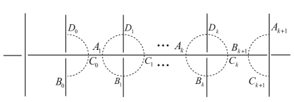
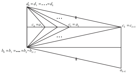
Figure 14: First non-alternating gluing and its cusp diagram ($k\geq 2$)

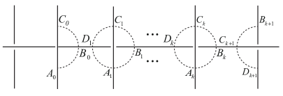
Figure 15: Second non-alternating gluing and its cusp diagram ($k\geq 2$)

Due to the completeness conditions in $\mathcal{H}$, the edges $d_{k}c_{k}$ and $b_{k}c_{k}$ are identified to $b_{k+1}a_{k+1}$ and $b_{k+1}c_{k+1}$ respectively in Figure 14(b), and the edges $a_{k}b_{k}$ and $c_{k}b_{k}$ are identified to $c_{k+1}d_{k+1}$ and $c_{k+1}b_{k+1}$ respectively in Figure 15(b). These identifications make the cusp diagrams topological annuli. Furthermore, due to the Thurston’s gluing equations of the edges in $\mathcal{C}\cup\mathcal{D}$, the annuli have Euclidean structures.

To complete the proof of Proposition 1.1, we show the completeness conditions in $\mathcal{H}$ and Thurston’s gluing equations of the the edges in $\mathcal{A}\cup\mathcal{C}\cup\mathcal{D}$ induce the other gluing equations of the edges in $\mathcal{B}$.

Consider the crossing $k$ in Figure 16. The crossing $l$ is the previous under-crossing of $k$ and the crossing $m$ is the next under-crossing.

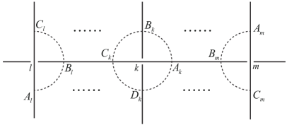
Figure 16: The case of ${\rm B}_{k}{\rm F}_{k}={\rm D}_{k}{\rm F}_{k}\in\mathcal{B}$

Thurston’s gluing equation of ${\rm B}_{k}{\rm F}_{k}={\rm D}_{k}{\rm F}_{k}\in\mathcal{B}$ follows from the gluing equation around $b_{k}=d_{k}$ of the cusp diagram in Figure 17 since $c_{l}d_{k}$ and $d_{k}a_{m}$ are parallel to $a_{l}b_{k}$ and $b_{k}c_{m}$ respectively.

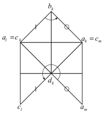
Figure 17: The cusp diagram of Figure 16

The proof of the case of ${\rm A}_{k}{\rm E}_{k}={\rm C}_{k}{\rm E}_{k}\in\mathcal{B}$ is also obtained by considering Figure 18 and following the same argument as before.

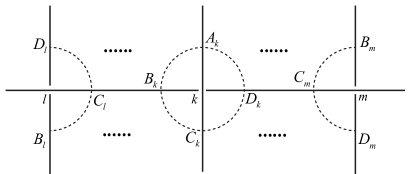
Figure 18: The case of ${\rm A}_{k}{\rm E}_{k}={\rm C}_{k}{\rm E}_{k}\in\mathcal{B}$

As a conclusion, we showed $\mathcal{H}$ induces Thurston’s gluing equations of all the edges. The completeness conditions along the meridian in $\mathcal{H}$ and all the gluing equations together induce the completeness condition along the longitude, so $\mathcal{H}$ induces the whole hyperbolicity equations.

∎

4 Proof of Theorem 1.2

In this section, we always assume ${\mathbb{z}}=(z_{1},\ldots,z_{n})$ is a solution in $\mathcal{S}_{j}$ and drop the index $j$ of $r_{j,k}$ in (6).

The main technique of the proof of Theorem 1.2 is the extended Bloch group theory in [20]. To apply it, we first define the vertex ordering of the octahedral triangulation. In Figure 6, we assign 0 and 1 to the vertices ${\rm E}_{k}$ and ${\rm F}_{k}$ respectively, 2 to the vertices ${\rm A}_{k}$ and ${\rm C}_{k}$, and 3 to the vertices ${\rm B}_{k}$ and ${\rm D}_{k}$. This assignment induces the vertex orderings of the four tetrahedra.

Note that the vertex ordering of each tetrahedron induces the orientations of the edges and the tetrahedron. The induced orientation of the tetrahedron can be different from the original orientation induced by the triangulation. For example, the tetrahedra ${\rm E}_{k}{\rm F}_{k}{\rm C}_{k}{\rm B}_{k}$ and ${\rm E}_{k}{\rm F}_{k}{\rm A}_{k}{\rm D}_{k}$ in Figure 6 are the cases. If the two orientations are the same, we define the sign of the tetrahedron $\sigma=1$, and if they are different, then $\sigma=-1$.

One important property of this vertex orientation is that when two edges are glued together in the triangulation, the orientations of the two edges induced by each vertex orderings coincide. (We call this condition edge-orientation consistency.) Because of this property, we can apply the formula in [20].

The triangulation we are using is an ideal triangulation, so we already parametrized all ideal tetrahedra of the triangulation by assigning shape parameters to horizontal edges in Section 3. For each tetrahedron with the vertex-orientation, we define an element of the extended pre-Bloch group $\sigma[u^{\sigma};p,q]\in\widehat{\mathcal{P}}(\mathbb{C})$, where $\sigma$ is the sign of the tetrahedron, $u$ is the shape parameter assigned to the edge connecting the $0$th and $1$st vertices, and $p,q$ are certain integers.

Zickert suggested a way to determine $p$ and $q$ from the developing map of the representation $\rho:\pi_{1}(M)\rightarrow{\rm PSL}(2,\mathbb{C})$ of a hyperbolic manifold $M$ in [20], and showed that

$$\widehat{L}(\sum\sigma[u^{\sigma};p,q])\equiv i({\rm vol}(\rho)+i\,{\rm cs}(\rho))~{}~{}({\rm mod}~{}\pi^{2}),$$ (10)

where the summation is over all tetrahedra and

$$\widehat{L}([u;p,q])={\rm Li}_{2}(u)-\frac{\pi^{2}}{6}+\frac{1}{2}q\pi i\log u+\frac{1}{2}\log(1-u)(\log u+p\pi i)$$

is a complex valued function defined on $\widehat{\mathcal{P}}(\mathbb{C})$.

Although our ideal triangulation $\mathcal{T}^{\prime}$ is that of $\mathbb{S}^{3}\backslash(L\cup\{\pm\infty\})$, the formula of [20] is still valid because of Thurston’s spinning construction. Theorem 4.11 of [20] already considered our case and the developing map of the representation is the one obtained by Thurston’s spinning construction. (The map sends $\pm\infty$ to ideal points corresponding to the trivial ends.)

To determine $p,q$ of $\sigma[u^{\sigma};p,q]$ of a tetrahedron with vertex orientation, we assign certain complex numbers $g_{jk}$ to the edge connecting the $j$th and $k$th vertices, where $j,k\in\{0,1,2,3\}$ and $j<k$. We assume $g_{jk}$ satisfies the property that if two edges are glued together in the triangulation, then the assigned $g_{jk}$’s of the edges coincide. We do not use the exact values of $g_{jk}$ in this article, but remark that there is an explicit method in [20] for calculating these numbers using the developing map. With the given numbers $g_{jk}$, we can calculate $p,q$ using the following equations, which appeared as equation (3.5) in [20]:

$$\left\{\begin{array}[]{ll}p\pi i=-\log u^{\sigma}+\log g_{03}+\log g_{12}-\log g_{02}-\log g_{13},\\ q\pi i=\log(1-u^{\sigma})+\log g_{02}+\log g_{13}-\log g_{23}-\log g_{01}.\end{array}\right.$$ (13)

To avoid confusion, we use variables $\alpha_{m},\beta_{m},\gamma_{m},\delta_{m}$ instead of $g_{jk}$. We assign $\alpha_{m}$ and $\beta_{m}$ to non-horizontal edges as in Figure 19, where $m=a,b,c,d$. We also assign $\gamma_{l}$ to horizontal edges and $\delta_{k}$ to the edge ${\rm E}_{k}{\rm F}_{k}$ inside the octahedron. Although we have $\alpha_{a}=\alpha_{c}$ and $\beta_{b}=\beta_{d}$, we use $\alpha_{a}$ for the tetrahedron ${\rm E}_{k}{\rm F}_{k}{\rm A}_{k}{\rm B}_{k}$ and ${\rm E}_{k}{\rm F}_{k}{\rm A}_{k}{\rm D}_{k}$, $\alpha_{c}$ for ${\rm E}_{k}{\rm F}_{k}{\rm C}_{k}{\rm B}_{k}$ and ${\rm E}_{k}{\rm F}_{k}{\rm C}_{k}{\rm D}_{k}$, $\beta_{b}$ for ${\rm E}_{k}{\rm F}_{k}{\rm A}_{k}{\rm B}_{k}$ and ${\rm E}_{k}{\rm F}_{k}{\rm C}_{k}{\rm B}_{k}$, $\beta_{d}$ for ${\rm E}_{k}{\rm F}_{k}{\rm C}_{k}{\rm D}_{k}$ and ${\rm E}_{k}{\rm F}_{k}{\rm A}_{k}{\rm D}_{k}$. We assign vertex orderings of the tetrahedra in Figure 19 by assigning 0 to ${\rm E}_{k}$, 1 to ${\rm F}_{k}$, 2 to ${\rm A}_{k}$ and ${\rm C}_{k}$, and 3 to ${\rm B}_{k}$ and ${\rm D}_{k}$. Then the orientation of the octahedral triangulation induced by this ordering satisfies the edge-orientation consistency.

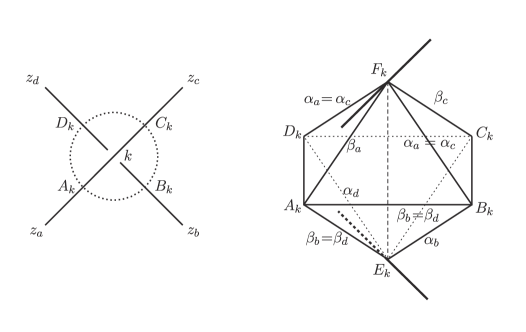
Figure 19: Labelings of non-horizontal edges

Observation 4.1.

For a fixed link diagram with the octahedral triangulation, we have

$$\log\alpha_{l}-\log\beta_{l}\equiv\log z_{l}+A~{}~{}({\rm mod}~{}\pi i),$$

for all $l=1,\ldots,n$, where $n$ is the number of sides of the diagram and $A$ is a complex constant number independent of $l$.

Proof.

Applying the definition of $p\pi i$ in (13) to the tetrahedra ${\rm E}_{k}{\rm F}_{k}{\rm A}_{k}{\rm B}_{k}$ and ${\rm E}_{k}{\rm F}_{k}{\rm C}_{k}{\rm B}_{k}$ in Figure 19, we have

$$\log z_{b}-\log z_{a} \equiv (\log\alpha_{b}-\log\beta_{b})-(\log\alpha_{a}-\log\beta_{a})~{}~{}({\rm mod}~{}\pi i),$$

$$\log z_{b}-\log z_{c} \equiv (\log\alpha_{b}-\log\beta_{b})-(\log\alpha_{c}-\log\beta_{c})~{}~{}({\rm mod}~{}\pi i).$$

Note that these equations hold for all tetrahedra in the triangulation. Therefore, by letting $A=(\log\alpha_{a}-\log\beta_{a})-\log z_{a}$, we complete the proof.

∎

Now we consider the three cases in Figure 10. For $m=a,b,c,d$, let $\sigma_{l}^{m}$ be the sign of the tetrahedron between the sides $z_{l}$ and $z_{m}$, and $u_{l}^{m}$ be the shape parameter of the tetrahedron assigned to the horizontal edge. We put $\tau_{l}^{m}=1$ when $z_{l}$ is the numerator of $(u_{l}^{m})^{\sigma_{l}^{m}}$ and $\tau_{l}^{m}=-1$ otherwise. We also define $p_{l}^{m}$ and $q_{l}^{m}$ so that $\sigma_{l}^{m}[(u_{l}^{m})^{\sigma_{l}^{m}};p_{l}^{m},q_{l}^{m}]$ becomes the element of $\widehat{\mathcal{P}}(\mathbb{C})$ corresponding to the tetrahedron. By definition, we know

$$u_{l}^{a}=\frac{z_{l}}{z_{a}},~{}u_{l}^{b}=\frac{z_{b}}{z_{l}},~{}u_{l}^{c}=\frac{z_{l}}{z_{c}},~{}u_{l}^{d}=\frac{z_{d}}{z_{l}}.$$ (14)

In the case (a) of Figure 10, we have

$$\sigma_{l}^{a}=1,~{}\sigma_{l}^{b}=1,~{}\sigma_{l}^{c}=-1,~{}\sigma_{l}^{d}=-1~{}\text{ and }~{}\tau_{l}^{a}=1,~{}\tau_{l}^{b}=-1,~{}\tau_{l}^{c}=-1,~{}\tau_{l}^{d}=1.$$

Using the equation (13) and Figure 20, we decide $p_{l}^{m}$ and $q_{l}^{m}$ as follows:

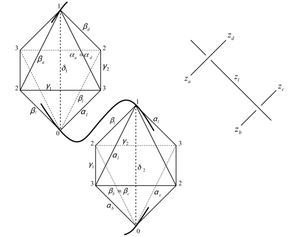
Figure 20: Case (a) of Figure 10

$$\left\{\begin{array}[]{ll}\log\frac{z_{l}}{z_{a}}+p_{l}^{a}\pi i=\log\alpha_{l}+\log\beta_{a}-\log\beta_{l}-\log\alpha_{a},\\ \log\frac{z_{b}}{z_{l}}+p_{l}^{b}\pi i=\log\alpha_{b}+\log\beta_{l}-\log\beta_{b}-\log\alpha_{l},\\ \log\frac{z_{c}}{z_{l}}+p_{l}^{c}\pi i=\log\alpha_{c}+\log\beta_{l}-\log\beta_{c}-\log\alpha_{l},\\ \log\frac{z_{l}}{z_{d}}+p_{l}^{d}\pi i=\log\alpha_{l}+\log\beta_{d}-\log\beta_{l}-\log\alpha_{d},\end{array}\right.$$ (19)

$$\left\{\begin{array}[]{ll}-\log(1-\frac{z_{l}}{z_{a}})+q_{l}^{a}\pi i=\log\beta_{l}+\log\alpha_{a}-\log\gamma_{1}-\log\delta_{1},\\ -\log(1-\frac{z_{b}}{z_{l}})+q_{l}^{b}\pi i=\log\beta_{b}+\log\alpha_{l}-\log\gamma_{1}-\log\delta_{2},\\ -\log(1-\frac{z_{c}}{z_{l}})+q_{l}^{c}\pi i=\log\beta_{c}+\log\alpha_{l}-\log\gamma_{2}-\log\delta_{2},\\ -\log(1-\frac{z_{l}}{z_{d}})+q_{l}^{d}\pi i=\log\beta_{l}+\log\alpha_{d}-\log\gamma_{2}-\log\delta_{1}.\end{array}\right.$$ (24)

In the case (b) of Figure 10, we have

$$\sigma_{l}^{a}=-1,~{}\sigma_{l}^{b}=1,~{}\sigma_{l}^{c}=-1,~{}\sigma_{l}^{d}=1~{}\text{ and }~{}\tau_{l}^{a}=\tau_{l}^{b}=\tau_{l}^{c}=\tau_{l}^{d}=-1.$$

Using the equation (13) and Figure 21, we decide $p_{l}^{m}$ and $q_{l}^{m}$ as follows:

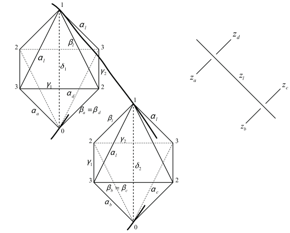
Figure 21: Case (b) of Figure 10

$$\left\{\begin{array}[]{ll}\log\frac{z_{a}}{z_{l}}+p_{l}^{a}\pi i=\log\alpha_{a}+\log\beta_{l}-\log\beta_{a}-\log\alpha_{l},\\ \log\frac{z_{b}}{z_{l}}+p_{l}^{b}\pi i=\log\alpha_{b}+\log\beta_{l}-\log\beta_{b}-\log\alpha_{l},\\ \log\frac{z_{c}}{z_{l}}+p_{l}^{c}\pi i=\log\alpha_{c}+\log\beta_{l}-\log\beta_{c}-\log\alpha_{l},\\ \log\frac{z_{d}}{z_{l}}+p_{l}^{d}\pi i=\log\alpha_{d}+\log\beta_{l}-\log\beta_{d}-\log\alpha_{l},\end{array}\right.$$ (29)

$$\left\{\begin{array}[]{ll}-\log(1-\frac{z_{a}}{z_{l}})+q_{l}^{a}\pi i=\log\beta_{a}+\log\alpha_{l}-\log\gamma_{1}-\log\delta_{1},\\ -\log(1-\frac{z_{b}}{z_{l}})+q_{l}^{b}\pi i=\log\beta_{b}+\log\alpha_{l}-\log\gamma_{1}-\log\delta_{2},\\ -\log(1-\frac{z_{c}}{z_{l}})+q_{l}^{c}\pi i=\log\beta_{c}+\log\alpha_{l}-\log\gamma_{2}-\log\delta_{2},\\ -\log(1-\frac{z_{d}}{z_{l}})+q_{l}^{d}\pi i=\log\beta_{d}+\log\alpha_{l}-\log\gamma_{2}-\log\delta_{1}.\end{array}\right.$$ (34)

In the case (c) of Figure 10, we have

$$\sigma_{l}^{a}=1,~{}\sigma_{l}^{b}=-1,~{}\sigma_{l}^{c}=1,~{}\sigma_{l}^{d}=-1~{}\text{ and }~{}\tau_{l}^{a}=\tau_{l}^{b}=\tau_{l}^{c}=\tau_{l}^{d}=1.$$

Using the equation (13) and Figure 22, we decide $p_{l}^{m}$ and $q_{l}^{m}$ as follows:

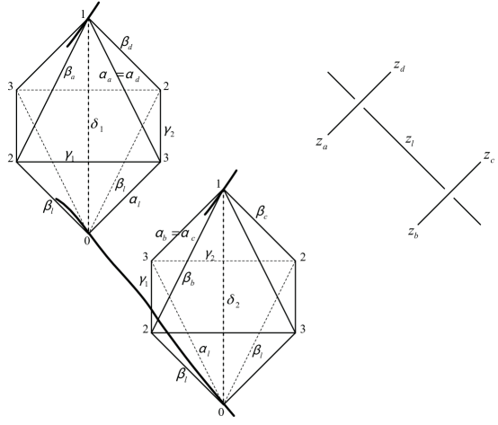
Figure 22: Case (c) of Figure 10

$$\left\{\begin{array}[]{ll}\log\frac{z_{l}}{z_{a}}+p_{l}^{a}\pi i=\log\alpha_{l}+\log\beta_{a}-\log\beta_{l}-\log\alpha_{a},\\ \log\frac{z_{l}}{z_{b}}+p_{l}^{b}\pi i=\log\alpha_{l}+\log\beta_{b}-\log\beta_{l}-\log\alpha_{b},\\ \log\frac{z_{l}}{z_{c}}+p_{l}^{c}\pi i=\log\alpha_{l}+\log\beta_{c}-\log\beta_{l}-\log\alpha_{c},\\ \log\frac{z_{l}}{z_{d}}+p_{l}^{d}\pi i=\log\alpha_{l}+\log\beta_{d}-\log\beta_{l}-\log\alpha_{d},\end{array}\right.$$ (39)

$$\left\{\begin{array}[]{ll}-\log(1-\frac{z_{l}}{z_{a}})+q_{l}^{a}\pi i=\log\beta_{l}+\log\alpha_{a}-\log\gamma_{1}-\log\delta_{1},\\ -\log(1-\frac{z_{l}}{z_{b}})+q_{l}^{b}\pi i=\log\beta_{l}+\log\alpha_{b}-\log\gamma_{1}-\log\delta_{2},\\ -\log(1-\frac{z_{l}}{z_{c}})+q_{l}^{c}\pi i=\log\beta_{l}+\log\alpha_{c}-\log\gamma_{2}-\log\delta_{2},\\ -\log(1-\frac{z_{l}}{z_{d}})+q_{l}^{d}\pi i=\log\beta_{l}+\log\alpha_{d}-\log\gamma_{2}-\log\delta_{1}.\end{array}\right.$$ (44)

Note that

$$\sigma_{l}^{m}=\sigma_{m}^{l},~{}\tau_{l}^{m}=-\tau_{m}^{l},~{}u_{l}^{m}=u_{m}^{l},~{}p_{l}^{m}=p_{m}^{l},~{}q_{l}^{m}=q_{m}^{l}\text{ and}$$

$$\sigma_{l}^{m}[(u_{l}^{m})^{\sigma_{l}^{m}};p_{l}^{m},q_{l}^{m}]=\sigma_{m}^{l}[(u_{m}^{l})^{\sigma_{m}^{l}};p_{m}^{l},q_{m}^{l}]\in\widehat{\mathcal{P}}(\mathbb{C}).$$

If we put the element $\frac{1}{2}\sum_{l,m}\sigma_{l}^{m}[(u_{l}^{m})^{\sigma_{l}^{m}};p_{l}^{m},q_{l}^{m}]\in\widehat{\mathcal{P}}(\mathbb{C})$ corresponding to the triangulation of $\mathbb{S}^{3}\backslash(L\cup\{\pm\infty\})$, the potential function defined in Section 2 can be expressed by the following way:

$$V(z_{1},\ldots,z_{n})=\frac{1}{2}\sum_{l,m}\sigma_{l}^{m}{\rm Li}_{2}\left((u_{l}^{m})^{\sigma_{l}^{m}}\right).$$

By direct calculation, we obtain

$$z_{l}\frac{\partial V}{\partial z_{l}}=-\sum_{m=a,\ldots,d}\sigma_{l}^{m}\tau_{l}^{m}\log(1-(u_{l}^{m})^{\sigma_{l}^{m}})$$ (45)

for all $l=1,\ldots,n$.

Recall that we use the notation $r_{k}$ instead of $r_{j,k}$, which was defined in (6).

Lemma 4.2.

For all $l=1,\ldots,n$, we have

$$r_{l}\pi i=-\sum_{m=a,\dots,d}\sigma_{l}^{m}\tau_{l}^{m}q_{l}^{m}\pi i.$$

Proof.

In the case (a) of Figure 10, using (6), (24), (45), $\alpha_{a}=\alpha_{d}$ and $\beta_{b}=\beta_{c}$, we can directly calculate the following:

$$r_{l}\pi i = z_{l}\frac{\partial V}{\partial z_{l}}=-\sum_{m=a,\ldots,d}\sigma_{l}^{m}\tau_{l}^{m}\log(1-(u_{l}^{m})^{\sigma_{l}^{m}})$$

$$= -q_{l}^{a}\pi i+q_{l}^{b}\pi i-q_{l}^{c}\pi i+q_{l}^{d}\pi i.$$

The cases (b) and (c) of Figure 10 also can be proved by the direct calculation using (34) and (44).

∎

Corollary 4.3.

For all possible $l$ and $m$, we have

$$\frac{1}{2}\sum_{l,m}\sigma_{l}^{m}q_{l}^{m}\pi i\log(u_{l}^{m})^{\sigma_{l}^{m}}\equiv-\sum_{l=1}^{n}r_{l}\pi i\log z_{l}~{}~{}({\rm mod}~{}2\pi^{2}).$$ (47)

Proof.

Note that $q_{l}^{m}$ is an integer. Using (14) and Lemma 4.2, we can directly calculate

$$\frac{1}{2}\sum_{l=1}^{n}\sum_{m=a,\ldots,d}\sigma_{l}^{m}q_{l}^{m}\pi i\log(u_{l}^{m})^{\sigma_{l}^{m}} \equiv \sum_{l=1}^{n}\left(\sum_{m=a,\ldots,d}\sigma_{l}^{m}\tau_{l}^{m}q_{l}^{m}\pi i\right)\log z_{l}~{}~{}({\rm mod}~{}2\pi^{2})$$

$$= -\sum_{l=1}^{n}r_{l}\pi i\log z_{l}.$$

∎

Lemma 4.4.

For all possible $l$ and $m$, we have

$$\frac{1}{2}\sum_{l,m}\sigma_{l}^{m}\log\left(1-(u_{l}^{m})^{\sigma_{l}^{m}}\right)\left(\log(u_{l}^{m})^{\sigma_{l}^{m}}+p_{l}^{m}\pi i\right)\equiv-\sum_{l=1}^{n}r_{l}\pi i\log z_{l}~{}~{}({\rm mod}~{}2\pi^{2}).$$

Proof.

Substituting the term $\left(\log(u_{l}^{m})^{\sigma_{l}^{m}}+p_{l}^{m}\pi i\right)$ to the summation of $\pm(\log\alpha_{k}-\log\beta_{k})$ terms by applying (19) or (29) or (39) and (4), we can verify

$$\frac{1}{2}\sum_{l,m}\sigma_{l}^{m}\log\left(1-(u_{l}^{m})^{\sigma_{l}^{m}}\right)\left(\log(u_{l}^{m})^{\sigma_{l}^{m}}+p_{l}^{m}\pi i\right)$$

$$=\sum_{l=1}^{n}\left(\sum_{m=a,\ldots,d}\sigma_{l}^{m}\tau_{l}^{m}\log(1-(u_{l}^{m})^{\sigma_{l}^{m}})\right)(\log\alpha_{l}-\log\beta_{l})$$

$$=-\sum_{l=1}^{n}r_{l}\pi i(\log\alpha_{l}-\log\beta_{l}).$$

Note that $r_{l}$ is an even integer and

$$z_{j}\frac{\partial{\rm Li}_{2}(z_{j}/z_{k})}{\partial z_{j}}+z_{k}\frac{\partial{\rm Li}_{2}(z_{j}/z_{k})}{\partial z_{k}}=-\log(1-\frac{z_{j}}{z_{k}})+\log(1-\frac{z_{j}}{z_{k}})=0$$

implies $\displaystyle\sum_{l=1}^{n}r_{l}\pi i=0.$ By using Observation 4.1 and the above property, we have

$$-\sum_{l=1}^{n}r_{l}\pi i(\log\alpha_{l}-\log\beta_{l})\equiv-\sum_{l=1}^{n}r_{l}\pi i(\log z_{l}+A)=-\sum_{l=1}^{n}r_{l}\pi i\log z_{l}~{}~{}({\rm mod}~{}2\pi^{2}).$$

∎

Combining (10), Corollary 4.3 and Lemma 4.4, we prove (4) as follows:

$$i({\rm vol}(\rho_{\mathbb{z}})+i\,{\rm cs}(\rho_{\mathbb{z}}))\equiv\widehat{L}\left(\frac{1}{2}\sum_{l,m}\sigma_{l}^{m}[(u_{l}^{m})^{\sigma_{l}^{m}};p_{l}^{m},q_{l}^{m}]\right)$$

$$=\frac{1}{2}\sum_{l,m}\sigma_{l}^{m}\left({\rm Li}_{2}\left((u_{l}^{m})^{\sigma_{l}^{m}}\right)-\frac{\pi^{2}}{6}\right)+\frac{1}{4}\sum_{l,m}\sigma_{l}^{m}q_{l}^{m}\pi i\log\left(u_{l}^{m}\right)^{\sigma_{l}^{m}}$$

$$~{}~{}+\frac{1}{4}\sum_{l,m}\sigma_{l}^{m}\log\left(1-\left(u_{l}^{m}\right)^{\sigma_{l}^{m}}\right)\left(\log\left(u_{l}^{m}\right)^{\sigma_{l}^{m}}+p_{l}^{m}\pi i\right)$$

$$\equiv V(z_{1},\ldots,z_{n})-\sum_{l=1}^{n}r_{l}\pi i\log z_{l}=V_{0}({\mathbb{z}})~{}~{}({\rm mod}~{}\pi^{2}).$$

The existence of a solution $\mathbb{z_{\infty}}$ satisfying ${\rm vol}(\rho_{\mathbb{z_{\infty}}})={\rm vol}(L)$ follows from Theorem 1.1 of [10]. Although this theorem was proved for closed manifolds, it is still true for our case because Thurston’s spinning construction and all the other steps of the proof are valid. From Thurston-Gromov-Goldman rigidity (Theorem 7.1 in [6]) and (4), we know $\rho_{\mathbb{z_{\infty}}}$ is the discrete and faithful representation and (5) holds. One minor remark is that Theorem 1.1 of [10] considered parameter space of Thurston’s gluing equations (without completeness condition), so $\mathbb{z_{\infty}}$ lies in the parameter space. However, because $\rho_{\mathbb{z_{\infty}}}$ is discrete and faithful, it is boundary-parabolic and $\mathbb{z_{\infty}}$ also satisfies the completeness condition. Therefore $\mathbb{z_{\infty}}\in\mathcal{S}$ and the path component of $\mathcal{S}$ containing $\mathbb{z_{\infty}}$ is $\mathcal{S}_{0}$.

5 Examples of the twist knots

Let $T_{n}$ ($n\geq 1$) be the twist knot with $n+3$ crossings in Figure 23. For example, $T_{1}$ is the figure-eight knot $4_{1}$ and $T_{2}$ is the $5_{2}$ knot. In this section, we show an application of Theorem 1.2 to the twist knot $T_{n}$ and several numerical results.

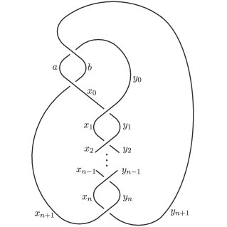
Figure 23: Twist knots $T_{n}$

We assign variables $a,b,x_{0},\ldots,x_{n+1},y_{0},\ldots,y_{n+1}$ to sides of Figure 23. Then the potential function becomes

$$V(T_{n};a,b,x_{0},\ldots,x_{n+1},y_{0},\ldots,y_{n+1})$$

$$=\left\{{\rm Li}_{2}(\frac{y_{0}}{b})-{\rm Li}_{2}(\frac{y_{0}}{y_{n+1}})+{\rm Li}_{2}(\frac{a}{y_{n+1}})-{\rm Li}_{2}(\frac{a}{b})\right\}$$

$$~{}~{}~{}+\left\{{\rm Li}_{2}(\frac{b}{x_{0}})-{\rm Li}_{2}(\frac{b}{a})+{\rm Li}_{2}(\frac{x_{n+1}}{a})-{\rm Li}_{2}(\frac{x_{n+1}}{x_{0}})\right\}$$

$$~{}~{}~{}+\sum_{k=0}^{n}\left\{{\rm Li}_{2}(\frac{y_{k+1}}{x_{k+1}})-{\rm Li}_{2}(\frac{y_{k+1}}{y_{k}})+{\rm Li}_{2}(\frac{x_{k}}{y_{k}})-{\rm Li}_{2}(\frac{x_{k}}{x_{k+1}})\right\}.$$

We abbreviate the notation of this function to $V(T_{n})$.

Finding the whole solution set of the hyperbolicity equations

$$\mathcal{H}(T_{n}):=\left\{\left.\exp(z\frac{\partial V(T_{n})}{\partial z})=1~{}\right|~{}z=a,b,x_{0},\ldots,x_{n+1},y_{0},\ldots,y_{n+1}\right\}$$

is neither easy nor useful. Instead, we can obtain enough solutions by fixing certain numbers, say $a=2$, $b=-1$ and $y_{n+1}=1$. Then, from $\exp(a\frac{\partial V(T_{n})}{\partial a})=1$, we find $x_{n+1}=3$.

If we denote $x_{0}=t$, then we can express all the other variables using $t$ as follows:

from $\exp(b\frac{\partial V(T_{n})}{\partial b})=1$, we find $y_{0}=1+\frac{2}{t}$. Also, from $\exp(x_{0}\frac{\partial V(T_{n})}{\partial x_{0}})=1$ and $\exp(y_{0}\frac{\partial V(T_{n})}{\partial y_{0}})=1$, we find $x_{1}=\frac{t(t+2)}{t^{2}-4t+8}$ and $y_{1}=\frac{4}{t}$.

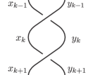
Figure 24: Crossings of the twist knot ($k=1,\ldots,n$)

For $k=1,\ldots,n$, the equations $\exp(x_{k}\frac{\partial V(T_{n})}{\partial x_{k}})=1$ and $\exp(y_{k}\frac{\partial V(T_{n})}{\partial y_{k}})=1$ of Figure 24 induce the following recursive formulas

$$x_{k+1}=\frac{x_{k}y_{k}}{-x_{k-1}+x_{k}+y_{k}},~{}y_{k+1}=x_{k}+y_{k}-\frac{x_{k}y_{k}}{y_{k-1}}.$$

They enable us to express all the variables in rational polynomials of $t$. Table 1 shows $x_{k}$ and $y_{k}$ in $t$ for $k=0,\ldots,5$.

$x_{0}$	$\displaystyle t$
$y_{0}$	$\displaystyle\frac{2+t}{t}$
$x_{1}$	$\displaystyle\frac{2t+t^{2}}{8-4t+t^{2}}$
$y_{1}$	$\displaystyle\frac{4}{t}$
$x_{2}$	$\displaystyle\frac{-4t}{-16+16t-7t^{2}+t^{3}}$
$y_{2}$	$\displaystyle\frac{32-16t+2t^{2}+t^{3}}{8t-4t^{2}+t^{3}}$
$x_{3}$	$\displaystyle\frac{32t-16t^{2}+2t^{3}+t^{4}}{128-192t+128t^{2}-40t^{3}+5t^{4}}$
$y_{3}$	$\displaystyle\frac{-64+64t-24t^{2}+t^{4}}{-16t+16t^{2}-7t^{3}+t^{4}}$
$x_{4}$	$\displaystyle\frac{-64t+64t^{2}-24t^{3}+t^{5}}{-256+512t-464t^{2}+224t^{3}-57t^{4}+6t^{5}}$
$y_{4}$	$\displaystyle\frac{512-768t+480t^{2}-112t^{3}-6t^{4}+5t^{5}}{128t-192t^{2}+128t^{3}-40t^{4}+5t^{5}}$
$x_{5}$	$\displaystyle\frac{512t-768t^{2}+480t^{3}-112t^{4}-6t^{5}+5t^{6}}{2048-5120t+5888t^{2}-3840t^{3}+1480t^{4}-316t^{5}+29t^{6}}$
$y_{5}$	$\displaystyle\frac{-1024+2048t-1792t^{2}+768t^{3}-124t^{4}-16t^{5}+6t^{6}}{-256t+512t^{2}-464t^{3}+224t^{4}-57t^{5}+6t^{6}}$

Table 1: $x_{k}$ and $y_{k}$ for $k=0,\dots,6$

Furthermore, $\exp(y_{n+1}\frac{\partial V(T_{n})}{\partial y_{n+1}})=1$ gives a simple relation

$$y_{n}=\frac{3t}{3t-4},$$ (48)

which determines the defining equation of $t$. Table 2 shows these equations for $n=1,\ldots,5$.

$n$	Defining equation of $t$
1	$16-12t+3t^{2}=0$
2	$-64+80t-40t^{2}+7t^{3}=0$
3	$256-448t+336t^{2}-120t^{3}+17t^{4}=0$
4	$-2048+4608t-4608t^{2}+2464t^{3}-696t^{4}+82t^{5}=0$
5	$4096-11264t+14080t^{2}-9984t^{3}+4192t^{4}-980t^{5}+99t^{6}=0$

Table 2: Defining equation (48) of $t$ for $n=1,\dots,5$

We checked all the solutions $t$ of the defining equation (48) in Table 2 satisfy the equations $\exp(x_{n}\frac{\partial V(T_{n})}{\partial x_{n}})=1$, $\exp(y_{n}\frac{\partial V(T_{n})}{\partial y_{n}})=1$ and $\exp(x_{n+1}\frac{\partial V(T_{n})}{\partial x_{n+1}})=1$. Therefore, all the solutions $t$ of the defining equation determine the solutions of $\mathcal{H}(T_{n})$. We denote the corresponding representation of $t$ by

$$\rho(T_{n})(t):\pi_{1}(\mathbb{S}^{3}\backslash T_{n})\longrightarrow{\rm PSL}(2,\mathbb{C}).$$

Then Table 3 shows the values of $t$ and the corresponding complex volumes of $\rho(T_{n})(t)$ for $n=1,\ldots,5$. Note that, when $n=2$, the values in Table 3 coincide with the result of the $5_{2}$ knot in Example 6.16 of [20].

$n$	$t$	$V_{0}(T_{n})(t)\equiv i({\rm vol}(\rho(T_{n})(t))+i\,{\rm cs}(\rho(T_{n})(t)))$
1	$t=2+1.1547...i$	$i(2.0299...+0\,i)$
	$t=2-1.1547...i$	$i(-2.0299...+0\,i)$
2	$t=1.4587...+1.0682...i$	$i(2.8281...+3.0241...i)$
	$t=1.4587...-1.0682...i$	$i(-2.8281...+3.0241...i)$
	$t=2.7969...$	$i(0-1.1135...i)$
3	$t=1.2631...+1.0347...i$	$i(3.1640...+6.7907...i)$
	$t=1.2631...-1.0347...i$	$i(-3.1640...+6.7907...i)$
	$t=2.2664...+0.7158...i$	$i(1.4151...+0.2110...i)$
	$t=2.2664...-0.7158...i$	$i(-1.4151...+0.2110...i)$
4	$t=1.1713...+1.0202...i$	$i(3.3317...+10.9583...i)$
	$t=1.1713...-1.0202...i$	$i(-3.3317...+10.9583...i)$
	$t=1.8097...+0.9073...i$	$i(2.2140...+1.8198...i)$
	$t=1.8097...-0.9073...i$	$i(-2.2140...+1.8198...i)$
	$t=2.5257...$	$i(0-0.8822...i)$
5	$t=1.1208...+1.0129...i$	$i(3.4272...+15.3545...i)$
	$t=1.1208...-1.0129...i$	$i(-3.4272...+15.3545...i)$
	$t=1.5498...+0.9676...i$	$i(2.6560...+4.6428...i)$
	$t=1.5498...-0.9676...i$	$i(-2.6560...+4.6428...i)$
	$t=2.2789...+0.4876...i$	$i(1.1087...-0.2581...i)$
	$t=2.2789...-0.4876...i$	$i(-1.1087...-0.2581...i)$

Table 3: Complex volumes of $\rho(T_{n})(t)$ for $n=1,\ldots,5$

Note that, from the well-known property (see Proposition 4.8 of [10] for example), the value $V_{0}(T_{n})(t)$ with the maximal imaginary part is the complex volume $i({\rm vol}(T_{n})+i\,{\rm cs}(T_{n}))$ of the hyperbolic knot $T_{n}$. We placed them at the top in Table 3.

We finally remark that the calculation method in this section also works for $n>5$ and finding complete solutions of $\mathcal{H}(T_{n})$ for small $n$ (and probably for all $n$) is possible. However, all the values of $V_{0}(T_{n})$ evaluated at the complete solutions lie in Table 3 for $n\leq 5$ (and probably do for any $n>5$ too). Therefore, our restricted solutions are general enough for calculating complex volumes of twist knots.

Acknowledgments The authors appreciate Yunhi Cho and Jun Murakami for discussions and suggestions on this work. The second author was supported by the Korea Research Foundation(KRF)grant funded by the Korea government(MEST)(No. 2013R1A1A2005861).

References

[1]
J. E. Andersen and R. Kashaev.
A TQFT from Quantum Teichmüller Theory.
Comm. Math. Phys., 330(3):887–934, 2014.
[2]
S. Baseilhac and R. Benedetti.
Quantum hyperbolic geometry.
Algebr. Geom. Topol., 7:845–917, 2007.
[3]
J. Cho.
Yokota theory, the invariant trace fields of hyperbolic knots and the
Borel regulator map.
arXiv:1005.3094.
[4]
J. Cho.
Optimistic limits of colored Jones polynomials and complex volumes
of hyperbolic links.
arXiv.org:1303.3701.
[5]
J. Cho and J. Murakami.
Optimistic limits of the colored Jones polynomials.
J. Korean Math. Soc., 50(3):641–693, 2013.
[6]
S. Francaviglia.
Hyperbolic volume of representations of fundamental groups of cusped
3-manifolds.
Int. Math. Res. Not., (9):425–459, 2004.
[7]
K. Hikami.
Generalized volume conjecture and the -polynomials: the
Neumann-Zagier potential function as a classical limit of the partition
function.
J. Geom. Phys., 57(9):1895–1940, 2007.
[8]
R. M. Kashaev.
The hyperbolic volume of knots from the quantum dilogarithm.
Lett. Math. Phys., 39(3):269–275, 1997.
[9]
F. Luo.
Volume optimization, normal surfaces, and Thurston’s equation on
triangulated 3-manifolds.
J. Differential Geom., 93(2):299–326, 2013.
[10]
F. Luo, S. Tillmann, and T. Yang.
Thurston’s spinning construction and solutions to the hyperbolic
gluing equations for closed hyperbolic 3-manifolds.
Proc. Amer. Math. Soc., 141(1):335–350, 2013.
[11]
R. Meyerhoff.
Density of the Chern-Simons invariant for hyperbolic
-manifolds.
In Low-dimensional topology and Kleinian groups
(Coventry/Durham, 1984), volume 112 of London Math. Soc. Lecture
Note Ser., pages 217–239. Cambridge Univ. Press, Cambridge, 1986.
[12]
H. Murakami.
Optimistic calculations about the Witten-Reshetikhin-Turaev
invariants of closed three-manifolds obtained from the figure-eight knot by
integral Dehn surgeries.
Sūrikaisekikenkyūsho Kōkyūroku, (1172):70–79, 2000.
Recent progress towards the volume conjecture (Japanese) (Kyoto,
2000).
[13]
H. Murakami and J. Murakami.
The colored Jones polynomials and the simplicial volume of a knot.
Acta Math., 186(1):85–104, 2001.
[14]
H. Murakami, J. Murakami, M. Okamoto, T. Takata, and Y. Yokota.
Kashaev’s conjecture and the Chern-Simons invariants of knots and
links.
Experiment. Math., 11(3):427–435, 2002.
[15]
W. D. Neumann and D. Zagier.
Volumes of hyperbolic three-manifolds.
Topology, 24(3):307–332, 1985.
[16]
H. Segerman and S. Tillmann.
Pseudo-developing maps for ideal triangulations I: essential edges
and generalised hyperbolic gluing equations.
In Topology and geometry in dimension three, volume 560 of Contemp. Math., pages 85–102. Amer. Math. Soc., Providence, RI, 2011.
[17]
J. Weeks.
Computation of hyperbolic structures in knot theory.
In Handbook of knot theory, pages 461–480. Elsevier B. V.,
Amsterdam, 2005.
[18]
Y. Yokota.
On the volume conjecture for hyperbolic knots.
arXiv:0009165.
[19]
Y. Yokota.
On the complex volume of hyperbolic knots.
J. Knot Theory Ramifications, 20(7):955–976, 2011.
[20]
C. K. Zickert.
The volume and Chern-Simons invariant of a representation.
Duke Math. J., 150(3):489–532, 2009.
Department of Mathematics, Korea Institute for Advanced Study (KIAS), Seoul 130-722, Republic of Korea
Department of Mathematical Sciences, Seoul National University, Seoul 151-747, Republic of Korea
Center for Geometry and Physics, Institute for Basic Science (IBS), Pohang 790-784, Republic of Korea