Sample Complexity of
Bayesian Optimal Dictionary Learning

Abstract

We consider a learning problem of identifying a dictionary matrix $\bm{D}\in\mathbb{R}^{M\times N}$ from a sample set of $M$ dimensional vectors $\bm{Y}\in\mathbb{R}^{M\times P}=N^{-1/2}\bm{D}\bm{X}\in\mathbb{R}^{M\times P}$, where $\bm{X}\in\mathbb{R}^{N\times P}$ is a sparse matrix in which the density of non-zero entries is $0<\rho<1$. In particular, we focus on the minimum sample size $P_{\rm c}$ (sample complexity) necessary for perfectly identifying $\bm{D}$ of the optimal learning scheme when $\bm{D}$ and $\bm{X}$ are independently generated from certain distributions. By using the replica method of statistical mechanics, we show that $P_{\rm c}\sim O(N)$ holds as long as $\alpha=M/N>\rho$ is satisfied in the limit of $N\to\infty$. Our analysis also implies that the posterior distribution given $\bm{Y}$ is condensed only at the correct dictionary $\bm{D}$ when the compression rate $\alpha$ is greater than a certain critical value $\alpha_{\rm M}(\rho)$. This suggests that belief propagation may allow us to learn $\bm{D}$ with a low computational complexity using $O(N)$ samples.

I Introduction

The concept of sparse representations has recently attracted considerable attention from various fields in which the number of measurements is limited. Many real-world signals such as natural images are represented sparsely in Fourier/wavelet domains; in other words, many components vanish or are negligibly small in amplitude when the signals are represented by Fourier/wavelet bases. This empirical property is exploited in the signal recovery paradigm of compressed sensing (CS), thereby enabling the recovery of sparse signals from much fewer measurements than those estimated by the Nyquist-Shannon sampling theorem [1, 2, 3, 4].

In signal processing techniques for exploiting sparsity, signals are generally assumed to be described as linear combinations of a few dictionary atoms. Therefore, the effectiveness of this approach is highly dependent on the choice of dictionary, by which the objective signals appear sparse. A method for choosing an appropriate dictionary for sparse representation is dictionary learning (DL), whereby the dictionary is constructed through a learning process from an available set of $P$ training samples [5, 6, 7, 8].

The ambiguity of the dictionary is fatal in signal/data analysis after learning. Therefore, an important issue is the estimation of the sample complexity, i.e., the sample size $P_{c}$ necessary for correct identification of the dictionary. In a seminal work, Aharon et al. showed that when the training set $\bm{Y}\in\mathbb{R}^{M\times P}$ is generated by a dictionary $\bm{D}\in\mathbb{R}^{M\times N}$ and a sparse matrix $\bm{X}\in\mathbb{R}^{N\times P}$ (planted solution) as $\bm{Y}=\bm{D}\bm{X}$, one can perfectly learn these if $P>P_{\rm c}=(k+1){}_{N}C_{k}$ and $k$ is sufficiently small, where $k$ is the number of non-zero elements in each column of $\bm{X}$ [9]. Unfortunately, this bound becomes exponentially large in $N$ for $k\sim O(N)$, which motivates us to improve the estimation. A recent study has shown that almost all dictionaries under the uniform measure are learnable with $P_{c}\sim O(NM)$ samples when $k\ln M\sim O(\sqrt{N})$ [10]. However, the fact that the number of unknown variables $MN+NP$ and known variables $MP$ are balanced with each other at $P\sim O(N)$ when $M\sim O(N)$ implies the possibility of DL with $O(N)$ training samples.

To answer this question, in this study, we evaluate the sample complexity of the optimal learning scheme defined for a given probabilistic model of dictionary learning. In a previous study, the authors assessed the sample complexity for a naive learning scheme: $\mathop{\rm min}_{\bm{D},\bm{X}}||\bm{Y}-\bm{D}\bm{X}||^{2}$ subj. to $||\bm{X}||_{0}\leq NP\rho$ $(0<\rho<1)$, where $||\bm{A}||$ indicates the Frobenius norm of $\bm{A}$, and $||\bm{X}||_{0}$ is the number of non-zero elements in $\bm{X}$ and $\bm{D}$ is enforced to be normalized appropriately. They used the replica method of statistical mechanics and found that $P_{\rm c}\sim O(N)$ holds when $\alpha=M/N$ is greater than a certain critical value $\alpha_{\rm naive}(\rho)>\rho$ [11]. However, the smallest possible $P_{\rm c}$ that can be obtained for $\alpha<\alpha_{\rm naive}(\rho)$ has not been clarified thus far. In this study, we show that $P_{\rm c}\sim O(N)$ holds in the entire region of $\alpha>\rho$ for the optimal learning scheme.

II Problem setup

Let us suppose the following scenario of dictionary learning. Planted solutions, an $M\times N$ dictionary matrix $\bm{D}\in\mathbb{R}^{M\times N}$ and an $N\times P$ sparse matrix $\bm{X}\in\mathbb{R}^{N\times P}$, are independently generated from prior distributions, $P(\bm{D})$ and $P_{\rho}(\bm{X})$, respectively, where $P(\bm{D})$ is the uniform distribution over an appropriate support and

$$P_{\rho}(\bm{X}) =\prod_{i,l}P_{\rho}(X_{il})\!=\!\prod_{i,l}\!\Big{\{}\!(1-\rho)\delta(X_{il})\!+\!\rho f(X_{il})\!\Big{\}}.$$ (1)

The rate of non-zero elements in $\bm{X}$ is given by $\rho\in[0,1]$, and the distribution function $f(X)$ does not have a finite mass probability at the origin. The set of training samples $\bm{Y}\in\mathbb{R}^{M\times P}$, whose column vector corresponds to a training sample, is assumed to be given by the planted solutions as

$$\bm{Y}=\frac{1}{\sqrt{N}}\bm{D}\bm{X},$$ (2)

where $1/\sqrt{N}$ is introduced for convenience in taking the large-system limit. A learner is required to infer $\bm{D}$ and $\bm{X}$ from $\bm{Y}$.

We impose the normalization constraint of $\sum_{\mu}D_{\mu i}^{2}=||\bm{D}_{i}||^{2}=M$ for each column $i=1\cdots,N$ to avoid the ambiguity of the product $\bm{DX}=\bm{DA}^{-1}\bm{AX}$ for diagonal matrices of positive diagonal entries $\bm{A}$. In addition, we introduce two other constraints that i) the values of $\sum_{\mu=1}^{M}D_{\mu i}$ are set to be positive and ii) columns of $\bm{D}$ are lined up in the descending order of the absolute value of $\sum_{\mu=1}^{M}D_{\mu i}$ so that ambiguities of simultaneous permutation and/or multiplication of same signs for columns in $\bm{D}$ and rows in $\bm{X}$ are removed. In the following, the uniform prior $P(\bm{D})$ is assumed to be defined on the support that satisfies all of these constraints.

Our aim is to evaluate the minimum value of the sample size $P$ required for perfectly identifying $\bm{D}$ and $\bm{X}$.

III Bayesian optimal learning

For mathematical formulation of our problem, let us denote the estimates of $\bm{D}$ and $\bm{X}$ yielded by an arbitrary learning scheme as $\hat{\bm{D}}(\bm{Y})$ and $\hat{\bm{X}}(\bm{Y})$. We evaluate the efficiency of the scheme using the mean squared errors (per element),

$${\rm MSE}_{D}(\hat{\bm{D}}(\cdot))\!=\!\frac{1}{NM}\!\sum_{\bm{Y},\bm{D},\bm{X}}\!P_{\rho}(\!\bm{D},\!\bm{X},\!\bm{Y}\!)||\bm{D}\!-\!\hat{\bm{D}}(\bm{Y})||^{2}$$ (3)

$${\rm MSE}_{X}(\hat{\bm{X}}(\cdot))\!=\!\frac{1}{NP}\!\sum_{\bm{Y},\bm{D},\bm{X}}\!P_{\rho}(\!\bm{D},\!\bm{X},\!\bm{Y}\!)||\bm{X}\!-\!\hat{\bm{X}}(\bm{Y})||^{2}$$ (4)

where $\bm{A}\cdot\bm{B}=\sum_{i,j}A_{ij}B_{ij}$ represents the inner product between two matrices of the same dimension $\bm{A}$ and $\bm{B}$. We impose the normalization constraint $\sum_{\mu=1}^{M}(\hat{\bm{D}}(\bm{Y}))_{\mu i}^{2}=M$ for each column index $i=1,2,\ldots,N$ in order to avoid the ambiguity of the product $\hat{\bm{D}}(\bm{Y})\hat{\bm{X}}(\hat{Y})=\hat{\bm{D}}(\bm{Y})\bm{A}^{-1}\bm{A}\hat{\bm{X}}({\bm{Y}})$ for an arbitrary invertible diagonal matrix $\bm{A}$. The joint distribution of $\bm{D}$, $\bm{X}$, and $\bm{Y}$ is given by

$$P_{\rho}(\bm{D},\bm{X},\bm{Y})=\delta(\bm{Y}-\frac{1}{\sqrt{N}}\bm{D}\bm{X})P(\bm{D})P_{\rho}(\bm{X}).$$ (5)

The perfect identification of $\bm{D}$ and $\bm{X}$ can be characterized by ${\rm MSE}_{D}={\rm MSE}_{X}=0$. The following theorem offers a useful basis for answering our question.

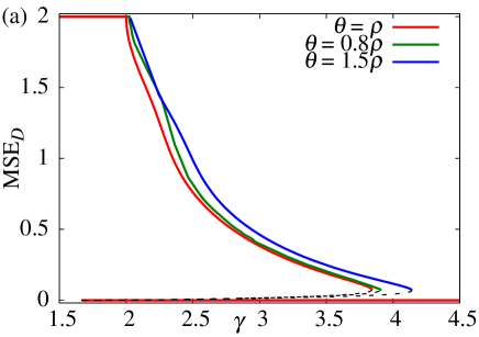
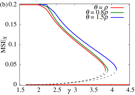
Figure 1: $\gamma$-dependence of (a) ${\rm MSE}_{D}$ and (b) ${\rm MSE}_{X}$ at $\alpha=0.5$, $\rho=0.2$. Plots for $\theta=\rho$, $0.8\rho$, and $1.5\rho$ show the optimality of the correct parameter choice $\theta=\rho$. Broken curves represent locally unstable branches, which are thermodynamically irrelevant.

Theorem 1.

For an arbitrary learning scheme, (3) and (4) are bounded from below as

$${\rm MSE}_{D}(\hat{\bm{D}}(\cdot))\geq 2-2\sum_{\bm{Y}}P_{\rho}(\bm{Y})\left(\frac{1}{N}\sum_{i=1}^{N}\frac{||(\langle\bm{D}\rangle_{\rho})_{i}||}{\sqrt{M}}\right)$$ (6)

$${\rm MSE}_{X}(\hat{\bm{X}}(\cdot))\geq\sum_{\bm{Y}}\!\ P_{\rho}(\bm{Y})\!\!\left(\frac{\left\langle\bm{X}\cdot\bm{X}\right\rangle_{\rho}}{NP}\!\!-\frac{\langle\bm{X}\rangle_{\rho}\!\cdot\!\langle\bm{X}\rangle_{\rho}}{NP}\right),$$ (7)

where $P_{\rho}(\bm{Y})=\sum_{\bm{D},\bm{X}}P_{\rho}(\bm{D},\bm{X},\bm{Y})$, and $\langle\cdot\rangle_{\rho}$ denotes the average over $\bm{D}$ and $\bm{X}$ according to the posterior distribution of $\bm{D}$ and $\bm{X}$ under a given $\bm{Y}$, $P_{\rho}(\bm{D},\bm{X}|\bm{Y})=P_{\rho}(\bm{D},\bm{X},\bm{Y})/P_{\rho}(\bm{Y})$. The equalities hold when the estimates satisfy

$$(\hat{\bm{D}}^{\rm opt}\!(\bm{Y}))_{i}=\sqrt{M}\frac{(\left\langle\bm{D}\right\rangle_{\rho})_{i}}{||(\left\langle\bm{D}\right\rangle_{\rho})_{i}||},~{}~{}\hat{\bm{X}}^{\rm opt}\!(\bm{Y})=\left\langle\bm{X}\right\rangle_{\rho},$$ (8)

where $(\bm{A})_{i}$ denotes the $i$-th column vector of matrix $\bm{A}$. We refer to (8) as the Bayesian optimal learning scheme [12].

Proof: By applying the Cauchy-Shwartz inequality and the minimization of the quadratic function to ${\rm MSE}_{D}$ and ${\rm MSE}_{X}$, respectively, one can obtain (6)–(8) after inserting the expression

$$\sum_{\bm{D},\bm{X}}xP\!\!_{\rho}(\bm{D}\!,\bm{X}\!,\bm{Y})\! =\!P\!\!_{\rho}(\bm{Y})\!\!\sum_{\bm{D},\bm{X}}\!\!xP\!\!_{\rho}(\bm{D}\!,\bm{X}|\bm{Y}\!)\!=\!P\!\!_{\rho}(\bm{Y})\!\left\langle x\right\rangle_{\rho}$$

for $x=\bm{D}$ and $\bm{X}$ into (3). $\Box$

This theorem guarantees that when the setup of dictionary learning is characterized by $P(\bm{D})$ and $P_{\rho}(\bm{X})$, the estimates of (8) offer the best possible learning performance in the sense that (3) and (4) are minimized. As the perfect identification of $\bm{D}$ and $\bm{X}$ is characterized by ${\rm MSE}_{D}={\rm MSE}_{X}=0$, our purpose is fulfilled by analyzing the performance of the Bayesian optimal learning scheme of (8).

IV Analysis

For simplicity of calculation, let us set $f(X_{il})$ as the Gaussian distribution with mean 0 and variance $\sigma_{X}^{2}$, and $\sigma_{X}^{2}$ is set to unity for all numerical calculations later on. For generality, we consider cases in which the sparsity assumed by the learner, denoted as $\theta$, can differ from the actual value $\rho$. When $\theta\neq\rho$, the estimates are given by $(\hat{\bm{D}}(\bm{Y}))_{i}=\sqrt{M}(\langle\bm{D}\rangle_{\theta})_{i}/||(\langle\bm{D}\rangle_{\theta})_{i}||$ and $\hat{\bm{X}}(\bm{Y})=\langle\bm{X}\rangle_{\theta}$ instead of (8). To evaluate ${\rm MSE}_{D}$ and ${\rm MSE}_{X}$, we need to evaluate macroscopic quantities

$$q_{D} \!=\!\frac{1}{MN}[\langle\bm{D}\rangle_{\theta}\!\!\cdot\!\langle\bm{D}\rangle_{\theta}]_{Y},~{}~{}m_{D}\!=\!\frac{1}{MN}[\langle\bm{D}\rangle_{\theta}\!\!\cdot\!\langle\bm{D}\rangle_{\rho}]_{Y}$$ (9)

$$Q_{X} =\frac{1}{NP}[\langle\bm{X}\!\cdot\!\bm{X}\rangle_{\theta}]_{Y}$$ (10)

$$q_{X} \!=\!\frac{1}{NP}[\langle\bm{X}\rangle_{\theta}\!\!\cdot\!\langle\bm{X}\rangle_{\theta}]_{Y},~{}~{}m_{X}\!=\!\frac{1}{NP}[\langle\bm{X}\rangle_{\theta}\!\!\cdot\!\langle\bm{X}\rangle_{\rho}]_{Y},$$ (11)

where $[\cdot]_{Y}=\sum_{\bm{Y}}P_{\rho}(\bm{Y})(\cdot)$. Note that (9)–(11) yield ${\rm MSE}_{D}\simeq 2-2m_{D}/\sqrt{q_{D}}$ and ${\rm MSE}_{X}=\rho\sigma_{X}^{2}+q_{X}-2m_{X}$.

Unfortunately, evaluating these is intrinsically difficult because it generally requires averaging the quantity

$$\frac{\sum_{\!\bm{D}^{1},\!\bm{X}^{1},\!\bm{D}^{2},\!\bm{X}^{2}}P_{\theta}(\bm{Y},\!\bm{D}^{1},\!\bm{X}^{1})P_{\theta}(\bm{Y},\!\bm{D}^{2},\!\bm{X}^{2})(\bm{D}^{1}\cdot\bm{D}^{2})}{\sum_{\!\bm{D}^{1},\!\bm{X}^{1},\!\bm{D}^{2},\!\bm{X}^{2}}P_{\theta}(\bm{Y},\!\bm{D}^{1},\!\bm{X}^{1})P_{\theta}(\bm{Y},\!\bm{D}^{2},\!\bm{X}^{2})}$$ (12)

$$(=\langle\bm{D}\rangle_{\theta}\!\!\cdot\!\langle\bm{D}\rangle_{\theta}),$$ (13)

which includes summations over exponentially many terms in the denominator, with respect to $\bm{Y}$. One promising approach for avoiding this difficulty involves multiplying $P_{\theta}^{n}(\bm{Y})=(\sum_{\bm{X},\bm{D}}P_{\theta}(\bm{Y},\bm{D},\bm{X}))^{n}$ $(n={2,3},\ldots\in\mathbb{N})$ inside the operation of $[\cdot]_{Y}$ for canceling the denominator of (13), which makes the evaluation of a modified average

$$q_{D}(n)=\frac{1}{MN}\frac{[P_{\theta}^{n}(\bm{Y})\langle\bm{D}\rangle_{\theta}\!\!\cdot\!\langle\bm{D}\rangle_{\theta}]_{Y}}{[P_{\theta}^{n}(\bm{Y})]_{Y}}$$ (14)

feasible via the saddle point assessment of $[P^{n}_{\theta}(\bm{Y})]_{Y}$ for $N,M,P\to\infty$, keeping $\alpha=M/N$ and $\gamma=P/N$ as $O(1)$. Furthermore, the resulting expression is likely to hold for $n\in\mathbb{R}$ as well. Therefore, we evaluate $q_{D}$ using the formula $q_{D}=\lim_{n\to 0}q_{D}(n)$ with the expression, and similarly, for $m_{D}$, $Q_{X}$, $q_{X}$, and $m_{X}$. This procedure is often termed the replica method [13, 14]. Under the replica symmetric ansatz, which assumes that the dominant saddle point in the evaluation is invariant under any permutation of replica indices $a=1,2,\ldots,n$, the assessment is reduced to evaluating the extremum of the free entropy (density) function

$$\phi =\gamma\Big{(}\frac{\hat{Q}_{X}Q_{X}+\hat{q}_{X}q_{X}}{2}-\hat{m}_{X}m_{X}+\langle\langle\ln\Xi_{X}\rangle\rangle\Big{)}$$

$$+\frac{\alpha}{2}\!\Big{(}\hat{Q}_{D}\!+\!\hat{q}_{D}q_{D}\!-\!2\hat{m}_{D}m_{D}\!-\!\ln(\hat{Q}_{D}\!+\!\hat{q}_{D})\!+\!\frac{\hat{q}_{D}\!+\!\hat{m}_{D}^{2}}{\hat{Q}_{D}\!+\!\hat{q}_{D}}\Big{)}$$

$$-\!\frac{\alpha\gamma}{2}\!\Big{\{}\!\frac{q_{D}q_{X}\!-\!2m_{D}m_{X}\!+\!\rho\sigma_{X}^{2}\!}{Q_{X}-q_{D}q_{X}}\!+\!\ln(Q_{X}\!-\!q_{D}q_{X})\Big{\}}\!,$$ (15)

where $\hat{\sigma}_{X}=1+(\hat{Q}_{X}+\hat{q}_{X})\sigma_{X}^{2}$,

$$\Xi_{X}\!\! =\!(1\!-\!\theta)\!+\!\frac{\theta}{\sqrt{\hat{\sigma}_{X}}}\exp\!\Big{(}\frac{\sigma_{X}^{2}(\sqrt{\hat{q}}_{X}z+\hat{m}_{X}X^{0})^{2}}{2\hat{\sigma}_{X}}\!\Big{)}$$

$$\equiv(1-\!\theta\!)+\!\Xi_{X}^{+},$$ (16)

and $\langle\langle\cdot\rangle\rangle$ denotes the average over $X$ and $z$, which are distributed according to $P_{\rho}(X)$ and a Gaussian distribution with mean zero and variance 1, respectively. The extremized value of $\phi$, $\phi^{*}$, is related to the average log-likelihood (density) of $\bm{Y}$ as $N^{-2}\sum_{\bm{Y}}P_{\rho}(\bm{Y})\ln P_{\theta}(\bm{Y})=\lim_{n\to 0}(\partial/\partial n)\left\{N^{-2}\ln[P_{\theta}^{n}(\bm{Y})]_{Y}\right\}=\phi^{*}+{\rm constant}.$

In Fig. 1, (a) ${\rm MSE}_{D}$ and (b) ${\rm MSE}_{X}$ for $\theta=\rho=0.2$ are plotted versus $\gamma$ together with those for $\theta=0.8\rho$ and $\theta=1.5\rho$. At $\theta=\rho$, ${\rm MSE}_{D}$ and ${\rm MSE}_{X}$ of thermodynamically relevant branches have minimum values in the entire $\gamma$ region, while a branch of solution characterized by ${\rm MSE}_{D}={\rm MSE}_{X}=0$ is shared by the three parameter sets. This supports the optimality of the correct parameter choice of $\theta=\rho$, and therefore, we hereafter focus our analysis on this case to estimate the minimum value of $\gamma$ for the perfect learning, ${\rm MSE}_{D}={\rm MSE}_{X}=0$. At $\theta=\rho$, the relationships $m_{D}=q_{D}$, $m_{X}=q_{X}$, and $Q_{X}=\rho$ hold from (9)–(11), and the extremum problem is reduced to

$$q_{D} \!=\!\frac{\hat{q}_{D}}{1+\hat{q}_{D}},~{}~{}q_{X}\!=\!\left<\left<\!\!\left(\frac{\Xi_{X}^{+}}{\Xi_{X}}\frac{\sqrt{\hat{q}_{X}}z+\hat{q}_{X}X^{0}}{\hat{\sigma}_{X}^{2}}\!\right)^{2}\right>\right>,$$ (17)

where $\hat{q}_{D}$ and $\hat{q}_{X}$ are given by

$$\hat{q}_{X}=\frac{\alpha q_{D}}{\rho\sigma_{X}^{2}-q_{D}q_{X}},~{}~{}~{}\hat{q}_{D}=\frac{\gamma q_{X}}{\rho\sigma_{X}^{2}-q_{D}q_{X}}.$$ (18)

The other variables are provided as $\hat{Q}_{D}=1$, $\hat{Q}_{X}=0$, $\hat{m}_{X}=\hat{q}_{X}$, and $\hat{m}_{D}=\hat{q}_{D}$.

V Results

V-A Actual solutions

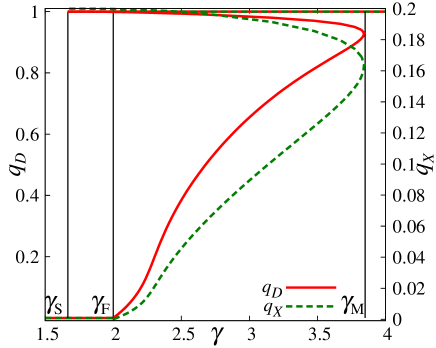
Figure 2: $\gamma$-dependence of $q_{D}$ (left axis) and $q_{X}$ (right axis) for $\alpha=0.5$ and $\rho=0.2$.

Fig. 2 plots $q_{D}$ and $q_{X}$ versus $\gamma$ for $\alpha=0.5$ and $\rho=0.2$. As shown in the figure, the solutions of $q_{D}$ and $q_{X}$ given by (17) are classified into three types: $q_{D}=1,~{}q_{X}=\rho{\sigma_{X}^{2}}$, $q_{D}=q_{X}=0$, and $0<q_{D}<1,~{}0<q_{X}<\rho{\sigma_{X}^{2}}$. The first one yields ${\rm MSE}_{D}={\rm MSE}_{X}=0$, indicating the correct identification of $\bm{D}$ and $\bm{X}$, and hence, we name it the success solution. The second one is referred to as the failure solution because it yields ${\rm MSE}_{D}=2$ and ${\rm MSE}_{X}=\rho\sigma_{X}^{2}$, which indicates complete failure of the learning of $\bm{D}$ and $\bm{X}$. The third one yields finite ${\rm MSE}_{D}$ and ${\rm MSE}_{X}$, $0<{\rm MSE}_{D}<2,~{}0<{\rm MSE}_{X}<\rho\sigma_{X}^{2}$, and we term it the middle solution.

V-A1 Success solution

When the expression

$$\delta\Big{(}\bm{Y}\!\!-\!\frac{\bm{DX}}{\sqrt{N}}\!\Big{)}\!=\!\lim_{\tau\to+0}\!\!\Big{(}\!\frac{1}{\sqrt{2\pi\tau}}\!\Big{)}^{MP}\!\!\!\!\!\!\!\!\exp\!\!\Big{(}\!\!-\!\frac{||\bm{Y}\!\!\!-\!\frac{1}{\sqrt{N}}\bm{DX}||^{2}}{2\tau}\!\Big{)},$$ (19)

is used, the success solution of $q_{D}$ and $q_{X}$ behaves as $(\rho\sigma_{X}^{2}-q_{X})/\tau=\chi_{X}$ and $(1-q_{D})/\tau=\chi_{D}$ while $\hat{q}_{X}$ and $\hat{q}_{D}$ scale as $\hat{q}_{X}=\hat{\theta}_{X}/\tau$ and $\hat{q}_{D}=\hat{\theta}_{D}/\tau$. By substituting them into the equations of $q_{D}$ and $q_{X}$, they are given by

$$\chi_{X}=\frac{\rho\gamma}{g},~{}~{}~{}\chi_{D}=\frac{\alpha}{\rho\sigma_{X}^{2}g},~{}~{}~{}\hat{\theta}_{X}=\frac{\rho}{\chi_{X}},~{}~{}~{}\hat{\theta}_{D}=\frac{1}{\chi_{D}},$$ (20)

where $g=(\alpha-\rho)\gamma-\alpha$. $\chi_{X}$ and $\chi_{D}$ must be positive by definition, and hence, the success solution exists for

$$\gamma>\frac{\alpha}{\alpha-\rho}\equiv\gamma_{\rm S}$$ (21)

only when $\alpha>\rho$.

V-A2 Failure solution

The failure solution $q_{D}=q_{X}=0$ appears at $0\leq\gamma<\gamma_{\rm F}$ as a locally stable solution. When $q_{D}$ and $q_{X}$ are sufficiently small, they are expressed as

$$q_{X} =\rho\sigma_{X}^{2}\alpha q_{D}+O(q^{2}),~{}~{}~{}q_{D}=\frac{\gamma q_{X}}{\rho\sigma_{X}^{2}}+O(q^{2}),$$ (22)

where $O(q^{2})$ denotes the higher-order terms over second-order with respect to $q_{D}$ and $q_{X}$. These expressions indicate that when

$$\gamma>\alpha^{-1}\equiv\gamma_{\rm F},$$ (23)

the local stability of $q_{D}=q_{X}=0$ is lost. As shown in Fig. 2, the failure solution vanishes at $\gamma_{\rm F}=2.0$ for $\alpha=0.5$.

V-A3 Middle solution

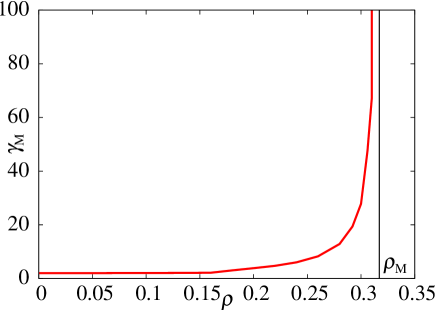
Figure 3: $\gamma_{\rm M}$ versus $\rho$ for $\alpha=0.5$.

We define $\gamma_{\rm M}$ over which the middle solution with $0<q_{D}<1$ and $0<q_{X}<\rho\sigma_{X}^{2}$ disappears, denoted as a vertical line in Fig. 2, which is provided as $\gamma_{\rm M}=3.841\ldots$ for the parameter choice of $(\alpha,\rho)=(0.5,0.2)$. The value of $\gamma_{\rm M}$ depends on $(\alpha,\rho)$, as shown in Fig. 3. This figure indicates that $\gamma_{\rm M}$ diverges at $\rho_{\rm M}=0.317\ldots$ for $\alpha=0.5$. The relation between $\rho_{\rm M}$ and $\alpha$, denoted as $\rho_{\rm M}(\alpha)$ (or $\alpha_{\rm M}(\rho)$), generally accords with the critical condition that belief propagation (BP)-based signal recovery using the correct prior starts to be involved with multiple fixed points for the signal reconstruction problem of compressed sensing [16] in which the correct dictionary $\bm{D}$ is provided in advance.

BP is also a potential algorithm for practically achieving the learning performance predicted by the current analysis because it is known that macroscopic behavior theoretically analyzed by the replica method can be confirmed experimentally for single instances by BP for many other systems [16, 17, 18]. The fact that only the success solution exists for $\gamma>\gamma_{\rm M}$ implies that one may be able to perfectly identify the correct dictionary $\bm{D}$ with a computational cost of polynomial order in $N$ utilizing BP, without being trapped by other locally stable solutions, for $\alpha>\alpha_{\rm M}(\rho)$.

V-B Free entropy density

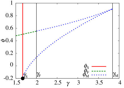
Figure 4: $\gamma$-dependence of $\phi$ for $\alpha=0.5$ and $\rho=0.2$. $\phi_{\rm S}$ diverges positively for $\gamma>\gamma_{\rm S}=\alpha/(\alpha-\rho)=1.666\ldots$.

There are three extrema of the free entropy (density), $\phi_{\rm S}$, $\phi_{\rm F}$, and $\phi_{\rm M}$, corresponding to the success solution, failure solution, and middle solution, respectively. Among them, the thermodynamically dominant solution that provides the correct evaluations of $q_{D}$ and $q_{X}$ is the one for which the value of free entropy is the largest. Fig. 4 plots $\phi_{\rm S}$, $\phi_{\rm F}$, and $\phi_{\rm M}$ versus $\gamma$ for $\alpha=0.5$, $\rho=0.2$, where $\gamma_{\rm S}=1.666\ldots$ and $\gamma_{\rm F}=2.0$. In particular, functional forms of $\phi_{\rm S}$ and $\phi_{\rm F}$ are given by

$$\phi_{\rm S}\! =\lim_{\tau\to+0}\!\frac{1}{2}\Big{[}g\!\left\{\ln(\frac{g}{\tau})\!-\!1\right\}\!-\!\alpha\gamma\ln(\alpha\gamma)\!+\!\alpha\!\left\{1\!-\!\ln\left(\frac{\rho\sigma_{X}^{2}}{\alpha}\right)\!\right\}$$

$$\hskip 28.45274pt\!+\!\gamma\rho(\ln\gamma-\ln\sigma_{X}^{2})\Big{]}\!-\!\gamma H(\rho)$$ (24)

$$\phi_{\rm F} =\frac{1}{2}\{-\alpha\gamma(1+\log\rho\sigma_{X}^{2})+\alpha\},$$ (25)

where $\tau\to+0$ originates from the expression of (19) and $H(\rho)=-(1-\rho)\log(1-\rho)-\rho\log(\rho)$. Further, (24) shows that $\phi_{\rm S}$ diverges positively for $g=(\alpha-\rho)\gamma-\alpha>0$, which guarantees that the success solution is always thermodynamically dominant for $\gamma>\gamma_{\rm S}=\alpha/(\alpha-\rho)$ as $\phi$ of other solutions is kept finite. This leads to the conclusion that the sample complexity of the Bayesian optimal learning is $P_{\rm c}=N\gamma_{\rm S}$, which is guaranteed as $O(N)$ as long as $\alpha>\rho$. This is the main consequence of the present study.

Fig. 5 plots the phase diagram in the $\alpha-\rho$ plane. The union of the regions (I) and (II) represents the condition that the sample complexity $P_{\rm c}$ is $O(N)$, while the full curve of the upper boundary of (II) denotes $\alpha_{\rm M}(\rho)$ above which BP is expected to work as an efficient learning algorithm. Dictionary learning is impossible in the region of (III). The critical condition $\alpha_{\rm{naive}}(\rho)$ above which the naive learning scheme of [11] can perfectly identify the planted solution by $O(N)$ samples is drawn as the dashed curve for comparison. The considerable difference between $\alpha_{\rm naive}(\rho)$ and $\rho$ (or even $\alpha_{\rm M}(\rho)$) indicates the significance of using adequate knowledge of probabilistic models in dictionary learning.

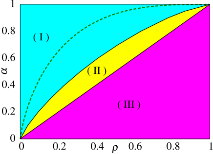
Figure 5: Phase diagram on $\alpha-\rho$ plane. The dashed curve in the area of (I) is the result of [11].

VI Summary

In summary, we assessed the minimum sample size required for perfectly identifying a planted solution in dictionary learning (DL). For this assessment, we derived the optimal learning scheme defined for a given probabilistic model of DL following the framework of Bayesian inference. Unfortunately, actually evaluating the performance of the Bayesian optimal learning scheme involves an intrinsic technical difficulty. For resolving this difficulty, we resorted to the replica method of statistical mechanics, and we showed that the sample complexity can be reduced to $O(N)$ as long as the compression rate $\alpha$ is greater than the density $\rho$ of non-zero elements of the sparse matrix. This indicates that the performance of a naive learning scheme examined in a previous study [11] can be improved significantly by utilizing the knowledge of adequate probabilistic models in DL. It was also shown that when $\alpha$ is greater than a certain critical value $\alpha_{\rm M}(\rho)$, the macroscopic state corresponding to perfect identification of the planted solution becomes a unique candidate for the thermodynamically dominant state. This suggests that one may be able to learn the planted solution with a computational complexity of polynomial order in $N$ utilizing belief propagation for $\alpha>\alpha_{\rm M}(\rho)$.
– Note added: After completing this study, the authors became aware that [19] presents results similar to those presented in this paper, where an algorithm for dictionary learning/calibration is independently developed on the basis of belief propagation.

References

- [1] J.-L. Starck, F. Murtagh , and J. M. Fadili, Sparse Image and Signal Processing: Wavelets, Curvelets, Morphological Diversity (Cambridge Univ. Press, New York, 2010).
- [2] H. Nyquist, Certain topics in telegraph transmission theory, Trans. AIEE 47 (2), pp. 617–644 (1928).
- [3] D. L. Donoho, Compressed sensing, IEEE Trans. Inform. Theory 52 (4), pp. 1289–1306 (2006).
- [4] E. J. Candès, and T Tao, Decoding by Linear Programming, IEEE Trans. Inform. Theory 51 (12), pp. 4203–4215 (2005).
- [5] B. A. Olshausen and D. J. Field, Sparse Coding with an Overcomplete Basis Set: A Strategy Employed by V1?, Vision Res. 37 (23), pp. 3311–3325 (1997).
- [6] R. Rubinstein, A. M. Bruckstein, and M. Elad, Dictionaries for Sparse Representation Modeling, Proc. of IEEE 98 (6), pp. 1045–1057 (2010).
- [7] M. Elad, Sparse and Redundant Representations: From Theory to Applications in Signal and Image Processing, (Springer-Verlag, New York, 2010).
- [8] S. Gleichman, and Y. C. Eldar, Blind Compressed Sensing, IEEE Inform. Theory 57, pp. 6958–6975 (2011).
- [9] M. Aharon, M. Elad, and A. M. Bruckstein, On the uniqueness of overcomplete dictionaries, and a practical way to retrieve them, Linear Algebra and its Applications 416 (1), pp. 48–67 (2006).
- [10] D. Vainsencher, S. Mannor, and A. M. Bruckstein, The Sample Complexity of Dictionary Learning, Journal of Machine Learning Research 12, pp. 3259–3281 (2011).
- [11] A. Sakata, and Y. Kabashima, Statistical mechanics of dictionary learning, arXiv:1203.6178.
- [12] Y. Iba, The Nishimori line and Bayesian statistics, J. Phys. A: Math. Gen. 32 (21), 3875–3888 (1999).
- [13] M. Mzard, G. Parisi, and M. A. Virasoro, Spin Glass Theory and Beyond, (World Sci. Pub., 1987).
- [14] H. Nishimori, Statistical Physics of Spin Glasses and Information Processing: An Introduction, (Oxford Univ. Pr., 2001).
- [15] M. Mézard and A. Montanari, Information, Physics, and Computation, (Oxford Univ. Press, Oxford, UK, 2009).
- [16] F. Krzakala, M. Mézard, F. Sausset, Y. F. Sun, and L. Zdeborová Statistical-Physics-Based Reconstruction in Compressed Sensing, Phys. Rev. X 2, pp. 021005-1–021005-18 (2012).
- [17] D. J. Thouless, P. W. Anderson, and R. G. Palmer, Solution of ’Solvable model of a spin glass, Phil. Mag. 35 (3), pp. 593–601 (1977).
- [18] K. Kabashima, A CDMA multiuser detection algorithm on the basis of belief propagation, J. Phys. A 36 (43), pp. 11111–11121 (2003).
- [19] F. Krzakala, M. Mézard, and L. Zdeborová, Phase Diagram and Approximate Message Passing for Blind Calibration and Dictionary Learning. Preprint received directly from the authors via private communication.