Analysis of the Discontinuous Petrov-Galerkin Method with Optimal Test Functions for the Reissner-Mindlin Plate Bending Model

Abstract

We analyze the discontinuous Petrov-Galerkin (DPG) method with optimal test functions when applied to solve the Reissner-Mindlin model of plate bending. We prove that the hybrid variational formulation underlying the DPG method is well-posed (stable) with a thickness-dependent constant in a norm encompassing the $L_{2}$-norms of the bending moment, the shear force, the transverse deflection and the rotation vector. We then construct a numerical solution scheme based on quadrilateral scalar and vector finite elements of degree $p$. We show that for affine meshes the discretization inherits the stability of the continuous formulation provided that the optimal test functions are approximated by polynomials of degree $p+3$. We prove a theoretical error estimate in terms of the mesh size $h$ and polynomial degree $p$ and demonstrate numerical convergence on affine as well as non-affine mesh sequences.

Keywords: plate bending; finite element method; discontinuous Petrov-Galerkin; discrete stability; optimal test functions; error estimates

1 Introduction

Finite element methods based on the principle of virtual displacements are the most widely used tools for computing the deformations and stresses of elastic bodies under external loads. However, in the modelling of thin-walled structures, the basic formulation leads to so-called locking, or numerical over-stiffness, unless special techniques (reduced integration, nonconforming elements) are applied, see [25, 24, 11, 7]. Another difficulty related to the displacement based formulations is the stress recovery. It is well known that the accuracy of the stress field derived from the displacement field can be much lower than that of the displacement field. Therefore special recovery techniques are often applied to improve the accuracy of stress approximations, see [33, 26]. Practical finite element design relies heavily on heuristics, intuition, and engineering expertise which make numerical analysis of the formulations difficult, since the various physical and geometrical assumptions do not have obvious interpretations in the functional analytic setting required for mathematical error analysis.

Mixed formulations where stresses are declared as independent unknowns are attractive because they often avoid the problem of locking by construction and allow direct approximation of the quantities of interest. However, in contrast to pure displacement formulations, mixed finite element methods do not inherit stability from the continuous formulation, but the stability of the discretization must be independently verified for each particular choice of finite element spaces as in [2, 30, 5, 13, 31, 14, 32, 4, 16]. The recently introduced discontinuous Petrov-Galerkin (DPG) variational framework provides means for automatic computation of test functions that guarantee discrete stability for any choice of trial functions, see [17, 18, 21, 27, 19, 20, 28, 35, 29].

In this paper we provide an error analysis for the DPG method with optimal test functions when applied to the Reissner-Mindlin model of plate bending. We follow the error analysis program laid down in [19, 23]. The stability analysis utilizes a duality argument based on the concept of optimal test space norm and is better suited to multidimensional problems than the earlier (see [18, 21, 27, 20]) analysis technique based on deriving an explicit expression for the generalized energy norm.

The unknowns in the (mesh-dependent) DPG formulation of the Reissner-Mindlin model are the shear force, bending moment, transverse deflection and rotation (field variables) as well as their suitable traces defined independently on the mesh skeleton. First, we show that the well-posedness and stability of the ideal DPG variational formulation follows from the well-posedness of the bending-moment formulation of the Reissner-Mindlin model which was established in [10], see also [1, 8, 9]. We introduce then a quadrilateral finite element discretization where the field variables are approximated by piecewise polynomial functions of degree $p$ or $p+1$ on each element and the traces by piecewise polynomials of degree $p$ (resultant tractions) and $p+1$ (displacements) on the mesh skeleton. We prove that on affine meshes the discrete formulation is stable in the sense of Babuška and Brezzi provided that the optimal test functions are approximated by piecewise polynomials of degree $p+3$ on each element.

The stability estimate is derived using regular (mesh and thickness independent) Sobolev norms and the estimate breaks down at the Kirchhoff limit corresponding to vanishing shear strains. Our final error bounds are therefore inversely proportional to the slenderness of the plate. The analysis indicates that the slenderness dependency arises from the shear stress term. This observation is corroborated by the numerical experiments which reveal that the accuracy of the shear stress is indeed affected by the value of the thickness while the other quantities are rather independent of it.

The paper is structured as follows. The derivation of the hybrid ultra-weak variational formulation of the Reissner-Mindlin plate bending model is presented in the next Section. The wellposedness of the formulation is proved in Section 3. The corresponding finite element method is introduced and analyzed in Section 4 and the results of our numerical experiments are shown in Section 5. The paper ends with conclusions and suggestions for future work in Section 6.

2 Reissner-Mindlin Plate Bending Model

2.1 Strong Form

Let $\Omega$ be a convex polygonal domain in $\mathbb{R}^{2}$ representing the middle surface of a plate. We take $L=\mathrm{diam}(\Omega)$ as the length unit and assume that the plate thickness $t$ is small as compared with unity, that is the plate is thin. In the Reissner-Mindlin model, the deformation of the plate is described in terms of the transverse deflection $w$ and the rotation vector $\boldsymbol{\psi}$, both defined on the middle surface $\Omega$. In the case of linearly elastic, homogeneous, and isotropic material, the shear force vector $\mathbf{V}$ and the bending moment tensor $\mathbf{M}$ are related to the displacements as (see for instance [34])

$$\mathbf{V}=\kappa Gt(\boldsymbol{\nabla}w-\boldsymbol{\psi}),\quad\mathbf{M}=Dt^{3}\left[(1-\nu)\boldsymbol{\varepsilon}(\boldsymbol{\psi})+\nu\operatorname{tr}(\boldsymbol{\varepsilon}(\boldsymbol{\psi}))\mathbf{I}\right],$$ (1)

where $\mathbf{I}$ is the identity tensor and $\boldsymbol{\varepsilon}(\boldsymbol{\psi})=\frac{1}{2}(\boldsymbol{\nabla}\boldsymbol{\psi}+\boldsymbol{\nabla}\boldsymbol{\psi}^{T})$ denotes the symmetric gradient. Moreover,

$$G=\frac{E}{2(1+\nu)},\quad D=\frac{E}{12(1-\nu^{2})}$$

are the elastic material parameters written in terms of Young’s modulus $E$ and Poisson’s ratio $\nu$ while $\kappa>0$ is an additional model parameter called the shear correction factor. The fundamental balance laws of static equilibrium are

$$-\boldsymbol{\nabla}\cdot\mathbf{V}=p,\quad-\boldsymbol{\nabla}\cdot\mathbf{M}-\mathbf{V}=\boldsymbol{0},$$ (2)

where $p$ represents a transversal bending load.

Upon rescaling the static quantities as

$$p\hookrightarrow Gt^{3}p,\quad\mathbf{V}\hookrightarrow Gt^{3}\mathbf{V},\quad\mathbf{M}\hookrightarrow Gt^{3}\mathbf{M},$$

introducing the auxiliary variable $\boldsymbol{\omega}=\frac{1}{2}(\boldsymbol{\nabla}\boldsymbol{\psi}-\boldsymbol{\nabla}\boldsymbol{\psi}^{T})$, and inverting the definition of $\mathbf{M}$ in (1) we arrive at the Reissner-Mindlin system

$$\kappa^{-1}t^{2}\mathbf{V}-\boldsymbol{\nabla}w+\boldsymbol{\psi} =\boldsymbol{0}, \qquad\mathcal{C}^{-1}\mathbf{M}-\boldsymbol{\nabla}\boldsymbol{\psi}+\boldsymbol{\omega} =\boldsymbol{0},$$ (3)

$$-\boldsymbol{\nabla}\cdot\mathbf{V} =p, \qquad-\boldsymbol{\nabla}\cdot\mathbf{M}-\mathbf{V} =\boldsymbol{0},$$

where

$$\mathcal{C}^{-1}\boldsymbol{\tau}=6\left(\boldsymbol{\tau}-\frac{\nu}{1+\nu}\operatorname{tr}(\boldsymbol{\tau})\mathbf{I}\right)$$

is the two-dimensional “compliance” tensor.

2.2 Hybrid Ultra-weak Form

We use the usual Sobolev spaces $H^{s}(X)$ of scalar-valued functions defined on a domain $X\subset\mathbb{R}^{2}$ and boldface font for the vector- and tensor-valued analogues. As usual, $H^{0}(X)=L_{2}(X)$. Accordingly, we make use of the space $H(\mathrm{div},X)$ consisting of vector fields in $\boldsymbol{L}_{2}(X)$ with divergence in $L_{2}(X)$ and denote by $\boldsymbol{H}(\mathbf{div},X)$ the corresponding space of tensor-valued functions with rows in $H(\mathrm{div},X)$ (the divergence of a tensor is taken row-wise).

Let $\{\Omega_{h}\}$ be a non-degenerate family of partitions of $\Omega$ into convex quadrilaterals, where $h$ refers to the maximum element diameter in $\Omega_{h}$. Integration of the system (3) by parts over a single element $K$ in $\Omega_{h}$ gives

$$\kappa^{-1}t^{2}(\mathbf{V},\mathbf{q})_{K}+(w,\boldsymbol{\nabla}\cdot\mathbf{q})_{K}-\langle w,\mathbf{q}\cdot\mathbf{n}\rangle_{\partial K}+(\boldsymbol{\psi},\mathbf{q})_{K} =0 \forall\mathbf{q}\in H(\mathrm{div},K)$$ (4)

$$(\mathcal{C}^{-1}\mathbf{M},\boldsymbol{\tau})_{K}+(\boldsymbol{\psi},\boldsymbol{\nabla}\cdot\boldsymbol{\tau})_{K}-\langle\boldsymbol{\psi},\boldsymbol{\tau}\mathbf{n}\rangle_{\partial K}+(r\mathbf{J},\boldsymbol{\tau})_{K} =0 \forall\,\boldsymbol{\tau}\in\boldsymbol{H}(\mathbf{div},K)$$

$$(\mathbf{V},\boldsymbol{\nabla}z)_{K}-\langle z,\mathbf{V}\cdot\mathbf{n}\rangle_{\partial K} =(p,z)_{K} \forall z\in H^{1}(K)$$

$$(\mathbf{M},\boldsymbol{\nabla}\boldsymbol{\phi})_{K}-\langle\boldsymbol{\phi},\mathbf{M}\mathbf{n}\rangle_{\partial K}-(\mathbf{V},\boldsymbol{\phi})_{K} =0 \forall\boldsymbol{\phi}\in\boldsymbol{H}^{1}(K)$$

$$(\mathbf{M},s\mathbf{J})_{K} =0 \forall s\in L_{2}(\Omega)$$

where $\mathbf{n}$ denotes the outward unit normal on $\partial K$. The standard $L_{2}$ inner product of scalar-, vector- or tensor-valued functions over $K$ and $\partial K$ have been denoted by $(\cdot,\cdot)_{K}$ and $\langle\cdot,\cdot\rangle_{\partial K}$, respectively. Moreover, the vorticity has been represented as a single unknown $\boldsymbol{\omega}=r\mathbf{J}$, where

$$\mathbf{J}=\begin{bmatrix}0&1\\ -1&0\end{bmatrix}$$

and the equilibrium condition $M_{12}=M_{21}$ has been imposed weakly using the same notation.

The next step in developing the DPG formulation is to declare the traces $(w,\boldsymbol{\psi},\mathbf{V}\cdot\mathbf{n},\mathbf{M}\mathbf{n})\!\!\mid_{\partial K}$ as indepedent unknowns by rewriting the boundary terms as

$$\langle w,\mathbf{q}\cdot\mathbf{n}\rangle_{\partial K} \hookrightarrow\langle\hat{w},\mathbf{q}\cdot\mathbf{n}\rangle_{1/2,\partial K}$$

$$\langle\boldsymbol{\psi},\boldsymbol{\tau}\mathbf{n}\rangle_{\partial K} \hookrightarrow\langle\hat{\boldsymbol{\psi}},\boldsymbol{\tau}\mathbf{n}\rangle_{1/2,\partial K}$$

$$\langle z,\mathbf{V}\cdot\mathbf{n}\rangle_{\partial K} \hookrightarrow\langle z,\hat{V}_{n}\rangle_{1/2,\partial K}$$

$$\langle\boldsymbol{\phi},\mathbf{M}\mathbf{n}\rangle_{\partial K} \hookrightarrow\langle\boldsymbol{\phi},\hat{\mathbf{M}}_{n}\rangle_{1/2,\partial K}$$

where $\langle\cdot,\ell\rangle_{1/2,\partial K}$ denotes the action of a functional $\ell$ in $H^{-1/2}$ acting on scalar- or vector-valued functions.

The boundary conditions for a clamped boundary are $\hat{\boldsymbol{\psi}}=\boldsymbol{0}$, $\hat{w}=0$ on $\partial\Omega$ and the final variational form of the problem is obtained by summing (4) over each $K$ in $\Omega_{h}$. The problem is to find $\mathbf{u}=(\mathbf{V},\mathbf{M},w,\boldsymbol{\psi},r,\hat{w},\hat{\boldsymbol{\psi}},\hat{V}_{n},\hat{\mathbf{M}}_{n})\in\boldsymbol{\mathcal{U}}$ such that

$$\mathcal{B}(\mathbf{u},\mathbf{v})=\mathcal{L}(\mathbf{v})\quad\forall\,\mathbf{v}=(\mathbf{q},\boldsymbol{\tau},z,\boldsymbol{\phi},s)\in\boldsymbol{\mathcal{V}}$$ (5)

where the functional spaces are defined formally as

$$\boldsymbol{\mathcal{U}} =\boldsymbol{L}_{2}(\Omega)\times\boldsymbol{L}_{2}(\Omega)\times L_{2}(\Omega)\times\boldsymbol{L}_{2}(\Omega)\times L_{2}(\Omega)$$ (6)

$$\times H_{0}^{1/2}(\partial\Omega_{h})\times\boldsymbol{H}^{1/2}_{0}(\partial\Omega_{h})\times H^{-1/2}(\partial\Omega_{h})\times\boldsymbol{H}^{-1/2}(\partial\Omega_{h})$$

$$\boldsymbol{\mathcal{V}} =H(\mathrm{div},\Omega_{h})\times\boldsymbol{H}(\mathbf{div},\Omega_{h})\times H^{1}(\Omega_{h})\times\boldsymbol{H}^{1}(\Omega_{h})\times L_{2}(\Omega)$$

and the bilinear and linear forms are given by

$$\mathcal{B}(\mathbf{u},\mathbf{v}) =(\mathbf{V},\kappa^{-1}t^{2}\mathbf{q}+\boldsymbol{\nabla}z-\boldsymbol{\phi})_{\Omega_{h}}+(\mathbf{M},\mathcal{C}^{-1}\boldsymbol{\tau}+\boldsymbol{\nabla}\boldsymbol{\phi}+s\mathbf{J})_{\Omega_{h}}$$ (7)

$$+(w,\boldsymbol{\nabla}\cdot\mathbf{q})_{\Omega_{h}}+(\boldsymbol{\psi},\mathbf{q}+\boldsymbol{\nabla}\cdot\boldsymbol{\tau})_{\Omega_{h}}+(r\mathbf{J},\boldsymbol{\tau})_{\Omega_{h}}-\langle\hat{w},\mathbf{q}\cdot\mathbf{n}\rangle_{\partial\Omega_{h}}-\langle\hat{\boldsymbol{\psi}},\boldsymbol{\tau}\mathbf{n}\rangle_{\partial\Omega_{h}}$$

$$-\langle z,\hat{V}_{n}\rangle_{\partial\Omega_{h}}-\langle\boldsymbol{\phi},\hat{\mathbf{M}}_{n}\rangle_{\partial\Omega_{h}}$$

$$\mathcal{L}(\mathbf{v}) =(p,z)_{\Omega_{h}}$$

Here we have adopted the notation of [23] for elementwise computations of the derivatives on the triangulation $\Omega_{h}$ and its skeleton $\partial\Omega_{h}$:

$$(\cdot,\cdot)_{\Omega_{h}}=\sum_{K\in\Omega_{h}}(\cdot,\cdot)_{K},\quad\langle\cdot,\cdot\rangle_{\partial\Omega_{h}}=\sum_{K\in\Omega_{h}}\langle\cdot,\cdot\rangle_{1/2,\partial K}$$

The broken Sobolev spaces in (6) are defined as

$$H^{1}(\Omega_{h}) =\{v\in L_{2}(\Omega)\;:\;v\!\!\mid_{K}\in H^{1}(K)\;\forall K\in\Omega_{h}\}$$

$$\boldsymbol{H}(\mathrm{div},\Omega_{h}) =\{\mathbf{q}\in\boldsymbol{L}_{2}(\Omega)\;:\;\mathbf{q}\!\!\mid_{K}\in\boldsymbol{H}(\mathrm{div},K)\;\forall K\in\Omega_{h}\}$$

whereas the fractional Sobolev spaces $H^{1/2}_{0}(\partial\Omega_{h})$ and $H^{-1/2}(\partial\Omega_{h})$ are interpreted as the trace spaces of functions in $H^{1}_{0}(\Omega)$ and $\boldsymbol{H}(\mathrm{div},\Omega)$ on the skeleton $\partial\Omega_{h}$:

$$H^{1/2}_{0}(\partial\Omega_{h}) =\{v\!\!\mid_{\partial\Omega_{h}}\;:\;v\in H^{1}_{0}(\Omega)\}$$

$$H^{-1/2}(\partial\Omega_{h}) =\{\boldsymbol{\eta}\cdot\mathbf{n}\!\!\mid_{\partial\Omega_{h}}\;:\;\boldsymbol{\eta}\in\boldsymbol{H}(\mathrm{div},\Omega)\}$$

The norms in the spaces $H^{1/2}_{0}(\partial\Omega_{h})$ and $H^{-1/2}(\partial\Omega_{h})$ can be defined as

$$||\hat{u}||_{H_{0}^{1/2}(\partial\Omega_{h})} =\inf_{v\in H^{1}_{0}(\Omega)}\{||v||_{H^{1}(\Omega)}:\gamma_{0}(v)=\hat{u}\}$$

$$||\hat{\eta}_{n}||_{H^{-1/2}(\partial\Omega_{h})} =\inf_{\boldsymbol{\eta}\in\boldsymbol{H}(\mathrm{div},\Omega)}\{||\boldsymbol{\eta}||_{\boldsymbol{H}(\mathrm{div},\Omega)}:\boldsymbol{\gamma}_{\mathbf{n}}(\boldsymbol{\eta})=\hat{\eta}_{n}\}$$

where $\gamma_{0}$ and $\boldsymbol{\gamma}_{\mathbf{n}}$ denote the trace operators satisfying $\gamma_{0}(v)=v\!\!\mid_{\partial\Omega_{h}}$ and $\boldsymbol{\gamma}_{\mathbf{n}}(\boldsymbol{\eta})=\boldsymbol{\eta}\cdot\mathbf{n}\!\!\mid_{\partial\Omega_{h}}$ for all $v\in\mathcal{C}^{1}(\bar{\Omega})$ and $\boldsymbol{\eta}\in\boldsymbol{\mathcal{C}}^{1}(\bar{\Omega})$, respectively.

3 Well-posedness of the Ultra-Weak Formulation

We begin with the following formulation of the Babuška-Lax-Milgram theorem and include the proof for completeness.

Theorem 3.1.

Assume that $\boldsymbol{\mathcal{U}}$ and $\boldsymbol{\mathcal{V}}$ are two Hilbert spaces and $\mathcal{B}(\mathbf{u},\mathbf{v})$ is a bilinear form on $\boldsymbol{\mathcal{U}}\times\boldsymbol{\mathcal{V}}$ satisfying

$$\mathcal{B}(\mathbf{u},\mathbf{v}) \leq C||\mathbf{u}||_{\boldsymbol{\mathcal{U}}}||\mathbf{v}||_{\boldsymbol{\mathcal{V}}}\quad\forall\mathbf{u}\in\boldsymbol{\mathcal{U}},\mathbf{v}\in\boldsymbol{\mathcal{V}}$$ (8)

$$\sup_{\mathbf{u}\in\boldsymbol{\mathcal{U}}}\frac{\mathcal{B}(\mathbf{u},\mathbf{v})}{||\mathbf{u}||_{\boldsymbol{\mathcal{U}}}} \geq\alpha||\mathbf{v}||_{\boldsymbol{\mathcal{V}}}\quad\forall\mathbf{v}\in\boldsymbol{\mathcal{V}}$$ (9)

$$\mathcal{B}(\mathbf{u},\mathbf{v}) =0\quad\forall\mathbf{v}\in\boldsymbol{\mathcal{V}}\quad\Rightarrow\quad\mathbf{u}=\boldsymbol{0}$$ (10)

If $\mathcal{L}\in\boldsymbol{\mathcal{V}}^{\prime}$, that is $\mathcal{L}$ is a linear functional on $\boldsymbol{\mathcal{V}}$, there exists a unique $\mathbf{u}\in\boldsymbol{\mathcal{U}}$ such that

$$\mathcal{B}(\mathbf{u},\mathbf{v})=\mathcal{L}(\mathbf{v})\quad\forall\mathbf{v}\in\boldsymbol{\mathcal{V}}$$

and

$$||\mathbf{u}||_{\boldsymbol{\mathcal{U}}}\leq\frac{||\mathcal{L}||}{\alpha}$$

Proof.

We show that the above assumptions guarantee that also the inf-sup condition

$$\sup_{\mathbf{v}\in\boldsymbol{\mathcal{V}}}\frac{\mathcal{B}{(\mathbf{u},\mathbf{v})}}{||\mathbf{v}||_{\boldsymbol{\mathcal{V}}}}\geq\alpha||\mathbf{u}||_{\boldsymbol{\mathcal{U}}}\quad\forall\mathbf{u}\in\boldsymbol{\mathcal{U}}$$ (11)

holds. The assertion follows then from the Babuška-Lax-Milgram Theorem, see [6, Theorem 2.1]. To prove (11) we define $\mathbf{T}:\boldsymbol{\mathcal{U}}\rightarrow\boldsymbol{\mathcal{V}}$ and $\mathbf{T}^{*}:\boldsymbol{\mathcal{V}}\rightarrow\boldsymbol{\mathcal{U}}$ through

$$\mathcal{B}(\mathbf{u},\mathbf{v})=(\mathbf{T}\mathbf{u},\mathbf{v})_{\boldsymbol{\mathcal{V}}}=(\mathbf{u},\mathbf{T}^{*}\mathbf{v})_{\boldsymbol{\mathcal{U}}}$$

It follows from (8) and the Riesz Representation Theorem that $\mathbf{T}$ and $\mathbf{T}^{*}$ are continuous and that (9) is equivalent to

$$||\mathbf{T}^{*}\mathbf{v}||_{\boldsymbol{\mathcal{U}}}\geq\alpha||\mathbf{v}||_{\boldsymbol{\mathcal{V}}}\quad\forall\mathbf{v}\in\boldsymbol{\mathcal{V}}$$ (12)

We show next that the range of $\mathbf{T}^{*}$ is closed. Namely, if $\{\mathbf{T}^{*}\mathbf{v}_{n}\}\in\boldsymbol{\mathcal{U}}$ is a Cauchy sequence, then so is $\{\mathbf{v}_{n}\}\in\boldsymbol{\mathcal{V}}$ because (9) implies that

$$||\mathbf{v}_{m}-\mathbf{v}_{n}||_{\boldsymbol{\mathcal{V}}}\leq\alpha||\mathbf{T}^{*}(\mathbf{v}_{m}-\mathbf{v}_{n})||_{\boldsymbol{\mathcal{U}}}=\alpha||\mathbf{T}^{*}\mathbf{v}_{m}-\mathbf{T}^{*}\mathbf{v}_{n}||_{\boldsymbol{\mathcal{U}}}$$

Therefore $\{\mathbf{v}_{n}\}$ converges to some $\mathbf{v}\in\boldsymbol{\mathcal{V}}$. Because $\mathbf{T}^{*}$ is continuous $\{\mathbf{T}^{*}\mathbf{v}_{n}\}$ converges to $\mathbf{T}^{*}\mathbf{v}$ which proves that $\overline{\mathbf{T}^{*}(\boldsymbol{\mathcal{V}})}=\mathbf{T}^{*}(\boldsymbol{\mathcal{V}})$.

The condition (10) implies now that $\mathbf{T}^{*}$ is surjective. If this was not true, there would exist a non-zero $\tilde{\mathbf{u}}\in\boldsymbol{\mathcal{U}}$ such $\mathcal{B}(\tilde{\mathbf{u}},\mathbf{v})=(\tilde{\mathbf{u}},\mathbf{T}^{*}\mathbf{v})=0$ for every $\mathbf{v}\in\boldsymbol{\mathcal{V}}$. However, this contradicts (10) so that we must have $\mathbf{T}^{*}(\boldsymbol{\mathcal{V}})=\boldsymbol{\mathcal{U}}$ which together with (12) implies (11):

$$\sup_{\mathbf{v}\in\boldsymbol{\mathcal{V}}}\frac{\mathcal{B}(\mathbf{u},\mathbf{v})}{||\mathbf{v}||_{\boldsymbol{\mathcal{V}}}}=\sup_{\mathbf{v}\in\boldsymbol{\mathcal{V}}}\frac{(\mathbf{u},\mathbf{T}^{*}\mathbf{v})_{\boldsymbol{\mathcal{U}}}}{||\mathbf{v}||_{\boldsymbol{\mathcal{V}}}}\geq\sup_{\mathbf{v}\in\boldsymbol{\mathcal{V}}}\frac{(\mathbf{u},\mathbf{T}^{*}\mathbf{v})_{\boldsymbol{\mathcal{U}}}}{\alpha^{-1}||\mathbf{T}^{*}\mathbf{v}||_{\boldsymbol{\mathcal{U}}}}=\alpha\sup_{\mathbf{w}\in\boldsymbol{\mathcal{U}}}\frac{(\mathbf{u},\mathbf{w})_{\boldsymbol{\mathcal{U}}}}{||\mathbf{w}||_{\boldsymbol{\mathcal{U}}}}=\alpha||\mathbf{u}||_{\boldsymbol{\mathcal{U}}}.$$

∎

3.1 Uniqueness of the Solution

Lemma 3.1.

Let the spaces $\boldsymbol{\mathcal{U}},\boldsymbol{\mathcal{V}}$ and the bilinear form $\mathcal{B}(\mathbf{u},\mathbf{v})$ be as defined in Equations (6) and (7), respectively. If $\mathbf{u}\in\boldsymbol{\mathcal{U}}$ satisfies

$$\mathcal{B}(\mathbf{u},\mathbf{v})=0$$ (13)

for every $\mathbf{v}\in\boldsymbol{\mathcal{V}}$, then $\mathbf{u}=\boldsymbol{0}$.

Proof.

Equation (13) implies that on every mesh element $K$ we have

$$\kappa^{-1}t^{2}(\mathbf{V},\mathbf{q})_{K}+(w,\boldsymbol{\nabla}\cdot\mathbf{q})_{K}-\langle\hat{w},\mathbf{q}\cdot\mathbf{n}\rangle_{\partial K}+(\boldsymbol{\psi},\mathbf{q})_{K} =0 \forall\mathbf{q}\in\boldsymbol{H}(\mathrm{div},K)$$ (14)

$$(\mathcal{C}^{-1}\mathbf{M},\boldsymbol{\tau})_{K}+(\boldsymbol{\psi},\boldsymbol{\nabla}\cdot\boldsymbol{\tau})_{K}-\langle\hat{\boldsymbol{\psi}},\boldsymbol{\tau}\mathbf{n}\rangle_{\partial K}+(r\mathbf{J},\boldsymbol{\tau})_{K} =0 \forall\boldsymbol{\tau}\in\boldsymbol{H}(\mathbf{div},K)$$

$$(\mathbf{V},\boldsymbol{\nabla}z)_{K}-\langle z,\hat{V}_{n}\rangle_{\partial K} =0 \forall z\in H^{1}(K)$$

$$(\mathbf{M},\boldsymbol{\nabla}\boldsymbol{\phi})_{K}-\langle\boldsymbol{\phi},\hat{\mathbf{M}}_{n}\rangle_{\partial K}-(\mathbf{V},\boldsymbol{\phi})_{K} =0 \forall\boldsymbol{\phi}\in\boldsymbol{H}^{1}(K)$$

$$(\mathbf{M},s\mathbf{J})_{K} =0 \forall s\in L_{2}(K)$$

Testing with infinitely differentiable functions which are non-zero only on a compact subset of $K$ reveals that

$$\kappa^{-1}t^{2}\mathbf{V}-\boldsymbol{\nabla}w+\boldsymbol{\psi} =\boldsymbol{0}$$ (15)

$$\mathcal{C}^{-1}\mathbf{M}-\boldsymbol{\nabla}\boldsymbol{\psi}+r\mathbf{J} =\boldsymbol{0}$$

$$-\boldsymbol{\nabla}\cdot\mathbf{V} =0$$

$$-\boldsymbol{\nabla}\cdot\mathbf{M}-\mathbf{V} =\boldsymbol{0}$$

in every $K$ in the distributional sense. These equations in turn imply that $\mathbf{V}\in\boldsymbol{H}(\mathrm{div},K)$, $\mathbf{M}\in\boldsymbol{H}(\mathbf{div},K)$ and $w\in H^{1}(K)$, $\boldsymbol{\psi}\in\boldsymbol{H}^{1}(K)$.

We also have

$$w\!\mid_{\partial K}=\hat{w}\!\mid_{\partial K},\;\boldsymbol{\psi}\!\mid_{\partial K}=\hat{\boldsymbol{\psi}}\!\mid_{\partial K}\quad\text{and}\quad\hat{V}_{n}\!\mid_{\partial K}=\mathbf{V}\cdot\mathbf{n}\!\mid_{\partial K},\;\hat{\mathbf{M}}_{n}\!\mid_{\partial K}=\mathbf{M}\mathbf{n}\!\mid_{\partial K}$$ (16)

This can be seen by integrating each equation in (14) by parts and using the corresponding identity in (15) to show that

$$\langle w-\hat{w},\mathbf{q}\cdot\mathbf{n}\rangle_{1/2,\partial K} =0 \forall\mathbf{q}\in\boldsymbol{H}(\mathrm{div},K)$$ (17)

$$\langle\boldsymbol{\psi}-\hat{\boldsymbol{\psi}},\boldsymbol{\tau}\mathbf{n}\rangle_{1/2,\partial K} =0 \forall\boldsymbol{\tau}\in\boldsymbol{H}(\mathbf{div},K)$$

$$\langle z,\mathbf{V}\cdot\mathbf{n}-\hat{V}_{n}\rangle_{1/2,\partial K} =0 \forall z\in H^{1}(K)$$

$$\langle\boldsymbol{\phi},\mathbf{M}\mathbf{n}-\hat{\mathbf{M}}_{n}\rangle_{1/2,\partial K} =0 \forall\boldsymbol{\phi}\in\boldsymbol{H}^{1}(K)$$

These equations imply that $\mathbf{M}\in\boldsymbol{H}(\mathbf{div},\Omega)$, $\mathbf{V}\in\boldsymbol{H}(\mathrm{div},\Omega)$, and that $w\in H^{1}_{0}(\Omega)$, $\boldsymbol{\psi}\in\boldsymbol{H}^{1}_{0}(\Omega)$ because $\hat{w}\!\mid_{\partial\Omega}=0$ and $\hat{\boldsymbol{\psi}}\!\mid_{\partial\Omega}=\boldsymbol{0}$.

The extra regularity allows us to set $\boldsymbol{\tau}=\mathbf{M}$, $\mathbf{q}=\mathbf{V}$ and $z=w$, $\boldsymbol{\phi}=\boldsymbol{\psi}$ in (14). Summing the equations together and over every element, we find after integration by parts and simplification that

$$\kappa^{-1}t^{2}(\mathbf{V},\mathbf{V})_{\Omega_{h}}+\langle w-\hat{w},\mathbf{V}\cdot\mathbf{n}\rangle_{\partial\Omega_{h}}+(\mathcal{C}^{-1}\mathbf{M},\mathbf{M})_{\Omega_{h}}+\langle\boldsymbol{\psi}-\hat{\boldsymbol{\psi}},\mathbf{M}\mathbf{n}\rangle_{\partial\Omega_{h}}-\langle w,\hat{V}_{n}\rangle_{\partial\Omega_{h}}-\langle\boldsymbol{\psi},\hat{\mathbf{M}}_{n}\rangle_{\partial\Omega_{h}}=0$$ (18)

The second and fourth terms vanish due to (17). The last two terms vanish as well. To see this, we use (16) and integrate by parts first locally and then globally (allowed by the regularity of $\mathbf{V},w,\mathbf{M},\boldsymbol{\psi}$) to find that

$$\langle w,\hat{V}_{n}\rangle_{\partial\Omega_{h}} =\langle w,\mathbf{V}\cdot\mathbf{n}\rangle_{\partial\Omega_{h}}$$ (19)

$$=(\boldsymbol{\nabla}w,\mathbf{V})_{\Omega_{h}}-(w,\boldsymbol{\nabla}\cdot\mathbf{V})_{\Omega_{h}}$$

$$=(\boldsymbol{\nabla}w,\mathbf{V})_{\Omega}-(w,\boldsymbol{\nabla}\cdot\mathbf{V})_{\Omega}$$

$$=\langle w,\mathbf{V}\cdot\mathbf{n}\rangle_{\partial\Omega}$$

Now the global boundary condition of $w\in H_{0}^{1}(\Omega)$ implies that $\langle w,\hat{V}_{n}\rangle_{\partial\Omega_{h}}=0$. A similar reasoning and the assumption $\boldsymbol{\psi}=\boldsymbol{H}_{0}^{1}(\Omega)$ show that $\langle\boldsymbol{\psi},\hat{\mathbf{M}}_{n}\rangle_{\partial\Omega_{h}}=0$.

Consequently, it follows from (18) that $\mathbf{V}$ and $\mathbf{M}$ must be zero. To proceed further, we recall (see for example [12, Section VI]) that for every $r\in L_{2}(\Omega)$, there exists a $\boldsymbol{\tau}^{r}\in\boldsymbol{H}(\mathbf{div},\Omega)$ such that $\boldsymbol{\nabla}\cdot\boldsymbol{\tau}^{r}=\boldsymbol{0}$ and $\tau^{r}_{12}-\tau^{r}_{21}=r$. We select $\boldsymbol{\tau}=\boldsymbol{\tau}^{r}$ in the second equation of (14) and sum over the elements to conclude as in (19) that

$$(r,r)_{\Omega_{h}} =\langle\hat{\boldsymbol{\psi}},\boldsymbol{\tau}^{r}\mathbf{n}\rangle_{\partial\Omega_{h}}=\langle\boldsymbol{\psi},\boldsymbol{\tau}^{r}\mathbf{n}\rangle_{\partial\Omega}=0$$

Thus, $r=0$.

Since $\mathbf{M}$ and $r$ are already known to vanish, the second equation in (15) implies that $\boldsymbol{\psi}$ is constant. Since $\boldsymbol{\psi}\in\boldsymbol{H}_{0}^{1}(\Omega)$ we find that $\boldsymbol{\psi}=\boldsymbol{0}$. The first equation in (15) implies then similarly that $w=0$. Finally (16) shows that also the traces $\hat{w}$, $\hat{\boldsymbol{\psi}}$ and $\hat{V}_{n}$, $\hat{\mathbf{M}}_{n}$ are zero. Thus, all components in $\mathbf{u}$ are shown to vanish and the proof is finished.

∎

3.2 Existence of the Solution

In the DPG terminology, the supremum in the condition (9) is called the optimal test space norm:

$$|||\mathbf{v}|||_{\boldsymbol{\mathcal{V}}}=\sup_{\mathbf{u}\in\boldsymbol{\mathcal{U}}}\frac{\mathcal{B}(\mathbf{u},\mathbf{v})}{||\mathbf{u}||_{\boldsymbol{\mathcal{U}}}}.$$

In the current application it can be expressed in the form

$$|||\mathbf{v}|||_{\boldsymbol{\mathcal{V}}}^{2} =||\kappa^{-1}t^{2}\mathbf{q}+\boldsymbol{\nabla}z-\boldsymbol{\phi}||_{\Omega_{h}}^{2}+||\mathcal{C}^{-1}\boldsymbol{\tau}+\boldsymbol{\nabla}\boldsymbol{\phi}+s\mathbf{J}||_{\Omega_{h}}^{2}+||\boldsymbol{\nabla}\cdot\mathbf{q}||_{\Omega_{h}}^{2}+||\mathbf{q}+\boldsymbol{\nabla}\cdot\boldsymbol{\tau}||_{\Omega_{h}}^{2}$$ (20)

$$+||\tau_{12}-\tau_{21}||_{\Omega_{h}}^{2}+||[\mathbf{q}\cdot\mathbf{n}]||_{\partial\Omega_{h}}^{2}+||[\boldsymbol{\tau}\mathbf{n}]||_{\partial\Omega_{h}}^{2}+||[z\mathbf{n}]||_{\partial\Omega_{h}}^{2}+||[\boldsymbol{\phi}\mathbf{n}]||_{\partial\Omega_{h}}^{2},$$

where $||\cdot||_{\Omega_{h}}^{2}=(\cdot,\cdot)_{\Omega_{h}}$ and

$$||[\mathbf{q}\cdot\mathbf{n}]||_{\partial\Omega_{h}} =\sup_{\hat{w}\in H^{1/2}_{0}(\partial\Omega_{h})}\frac{\langle\hat{w},\mathbf{q}\cdot\mathbf{n}\rangle_{\partial\Omega_{h}}}{||\hat{w}||_{H^{1/2}(\partial\Omega_{h})}},\quad ||[\boldsymbol{\tau}\mathbf{n}]||_{\partial\Omega_{h}} =\sup_{\hat{\boldsymbol{\psi}}\in\boldsymbol{H}^{1/2}_{0}(\partial\Omega_{h})}\frac{\langle\hat{\boldsymbol{\psi}},\boldsymbol{\tau}\mathbf{n}\rangle_{\partial\Omega_{h}}}{||\hat{\boldsymbol{\psi}}||_{\boldsymbol{H}^{1/2}(\partial\Omega_{h})}},$$

$$||[z\mathbf{n}]||_{\partial\Omega_{h}} =\sup_{\hat{V}_{n}\in H^{-1/2}(\partial\Omega_{h})}\frac{\langle z,\hat{V}_{n}\rangle_{\partial\Omega_{h}}}{||\hat{V}_{n}||_{H^{-1/2}(\partial\Omega_{h})}},\quad ||[\boldsymbol{\phi}\mathbf{n}]||_{\partial\Omega_{h}} =\sup_{\hat{\mathbf{M}}_{n}\in\boldsymbol{H}^{-1/2}(\partial\Omega_{h})}\frac{\langle\boldsymbol{\phi},\hat{\mathbf{M}}_{n}\rangle_{\partial\Omega_{h}}}{||\hat{\mathbf{M}}_{n}||_{\boldsymbol{H}^{-1/2}(\partial\Omega_{h})}}.$$

It is easy to see that conditions (9) and (8) of the Babuška-Lax-Milgram Theorem are equivalent to the following Lemma.

Lemma 3.2.

There exist positive constants $\alpha$ and $C$, which are independent of the mesh $\Omega_{h}$, such that

$$\alpha||\mathbf{v}||_{\boldsymbol{\mathcal{V}}}\leq|||\mathbf{v}|||_{\boldsymbol{\mathcal{V}}}\leq C||\mathbf{v}||_{\boldsymbol{\mathcal{V}}}\quad\forall\mathbf{v}\in\boldsymbol{\mathcal{V}}.$$ (21)

Proof.

Let $\mathbf{v}=(\mathbf{q},\boldsymbol{\tau},z,\boldsymbol{\phi},s)\in\boldsymbol{\mathcal{V}}$ be given and denote by

$$(\mathbf{V},\mathbf{M},w,\boldsymbol{\psi},r)\in\boldsymbol{H}(\mathrm{div},\Omega)\times\boldsymbol{H}(\mathbf{div},\Omega)\times L_{2}(\Omega)\times\boldsymbol{L}_{2}(\Omega)\times L_{2}(\Omega)$$

the solution to the variational problem

$$\kappa^{-1}t^{2}(\mathbf{V},\delta\mathbf{V})_{\Omega}+(w,\boldsymbol{\nabla}\cdot\delta\mathbf{V})_{\Omega}+(\boldsymbol{\psi},\delta\mathbf{V})_{\Omega} =(\mathbf{q},\delta\mathbf{V})_{\Omega} \forall\delta\mathbf{V}\in\boldsymbol{H}(\mathrm{div},\Omega),$$ (22)

$$(\mathcal{C}^{-1}\mathbf{M},\delta\mathbf{M})_{\Omega}+(\boldsymbol{\psi},\boldsymbol{\nabla}\cdot\delta\mathbf{M})_{\Omega}+(r\mathbf{J},\delta\mathbf{M})_{\Omega} =(\boldsymbol{\tau},\delta\mathbf{M})_{\Omega} \forall\delta\mathbf{M}\in\boldsymbol{H}(\mathbf{div},\Omega),$$

$$(-\boldsymbol{\nabla}\cdot\mathbf{V},\delta w)_{\Omega} =(z,\delta w)_{\Omega} \forall\delta w\in L_{2}(\Omega),$$

$$(-\boldsymbol{\nabla}\cdot\mathbf{M}-\mathbf{V},\delta\boldsymbol{\psi})_{\Omega} =(\boldsymbol{\phi},\delta\boldsymbol{\psi})_{\Omega} \forall\delta\boldsymbol{\psi}\in\boldsymbol{L}_{2}(\Omega),$$

$$(\mathbf{M},\delta r\mathbf{J})_{\Omega} =(s,\delta r)_{\Omega} \forall\delta r\in L_{2}(\Omega),$$

which exists and is unique due to the wellposedness of the bending moment formulation of the Reissner-Mindlin model. Namely, the analysis of [10] shows that the bilinear form induced by the left hand side of (22) satisfies the inf-sup condition in a norm encompassing

$$t||\mathbf{V}||_{\boldsymbol{L}_{2}(\Omega)},\;||\boldsymbol{\nabla}\cdot\mathbf{V}||_{\boldsymbol{L}_{2}(\Omega)},\;||\mathbf{M}||_{\boldsymbol{L}_{2}(\Omega)},\;||\boldsymbol{\nabla}\cdot\mathbf{M}+\mathbf{V}||_{\boldsymbol{L}_{2}(\Omega)},\;||w||_{L_{2}(\Omega)},\;||\boldsymbol{\psi}||_{\boldsymbol{L}_{2}(\Omega)},\;||r||_{L_{2}(\Omega)}.$$ (23)

Testing with infinitely smooth functions in the first two equations of (22) reveals then that $w\in H^{1}(\Omega)$, $\boldsymbol{\psi}\in\boldsymbol{H}^{1}(\Omega)$ so that the solution of (22) satisfies the estimate

$$t||\mathbf{V}||_{\boldsymbol{L}_{2}(\Omega)}+||\boldsymbol{\nabla}\cdot\mathbf{V}||_{L_{2}(\Omega)} +||\mathbf{M}||_{\boldsymbol{L}_{2}(\Omega)}+||\boldsymbol{\nabla}\cdot\mathbf{M}+\mathbf{V}||_{\boldsymbol{L}_{2}(\Omega)}+||w||_{H^{1}(\Omega)}+||\boldsymbol{\psi}||_{\boldsymbol{H}^{1}(\Omega)}+||r||_{\boldsymbol{L}_{2}(\Omega)}$$ (24)

$$\leq C\left(||\mathbf{q}||_{\boldsymbol{L}_{2}(\Omega)}+||\boldsymbol{\tau}||_{\boldsymbol{L}_{2}(\Omega)}+||z||_{L_{2}(\Omega)}+||\boldsymbol{\phi}||_{\boldsymbol{L}_{2}(\Omega)}+||s||_{L_{2}(\Omega)}\right)$$

where the constant $C>0$ is independent of $t$, $\mathbf{q}$, $\boldsymbol{\tau}$, $z$, $\boldsymbol{\phi}$, and $s$.

The passage from (14) to (15) can be repeated to arrive from (22) to the system

$$\kappa^{-1}t^{2}\mathbf{V}-\boldsymbol{\nabla}w+\boldsymbol{\psi} =\mathbf{q}$$ (25)

$$\mathcal{C}^{-1}\mathbf{M}-\boldsymbol{\nabla}\boldsymbol{\psi}+r\mathbf{J} =\boldsymbol{\tau}$$

$$-\boldsymbol{\nabla}\cdot\mathbf{V} =z$$

$$-\boldsymbol{\nabla}\cdot\mathbf{M}-\mathbf{V} =\boldsymbol{\phi}$$

valid on each $K$ in the distributional sense. Now integration by parts yields

$$||\mathbf{q}||_{\boldsymbol{L}_{2}(\Omega)}^{2}+||\boldsymbol{\tau}||_{\boldsymbol{L}_{2}(\Omega)}^{2}+||z||_{L_{2}(\Omega)}^{2} +||\boldsymbol{\phi}||_{\boldsymbol{L}_{2}(\Omega)}^{2}+||s||_{L_{2}(\Omega)}^{2}$$

$$=(\kappa^{-1}t^{2}\mathbf{V}-\boldsymbol{\nabla}w+\boldsymbol{\psi},\mathbf{q})_{\Omega}+(\mathcal{C}^{-1}\mathbf{M}-\boldsymbol{\nabla}\boldsymbol{\psi}+r\mathbf{J},\boldsymbol{\tau})_{\Omega}$$

$$\quad-(\boldsymbol{\nabla}\cdot\mathbf{V},z)_{\Omega}-(\boldsymbol{\nabla}\cdot\mathbf{M}+\mathbf{V},\boldsymbol{\phi})_{\Omega}+(\mathbf{M},s\mathbf{J})_{\Omega}$$

$$=\kappa^{-1}t^{2}(\mathbf{V},\mathbf{q})_{\Omega_{h}}+(w,\boldsymbol{\nabla}\cdot\mathbf{q})_{\Omega_{h}}-\langle w,\mathbf{q}\cdot\mathbf{n}\rangle_{\partial\Omega_{h}}+(\boldsymbol{\psi},\mathbf{q})_{\Omega_{h}}$$

$$\quad+(\mathcal{C}^{-1}\mathbf{M},\boldsymbol{\tau})_{\Omega_{h}}+(\boldsymbol{\psi},\boldsymbol{\nabla}\cdot\boldsymbol{\tau})_{\Omega_{h}}-\langle\boldsymbol{\psi},\boldsymbol{\tau}\mathbf{n}\rangle_{\partial\Omega_{h}}+(r\mathbf{J},\boldsymbol{\tau})_{\Omega_{h}}$$

$$\quad+(\mathbf{V},\boldsymbol{\nabla}z)_{\Omega_{h}}-\langle z,\mathbf{V}\cdot\mathbf{n}\rangle_{\partial\Omega_{h}}$$

$$\quad+(\mathbf{M},\boldsymbol{\nabla}\boldsymbol{\phi})_{\Omega_{h}}-\langle\boldsymbol{\phi},\mathbf{M}\mathbf{n}\rangle_{\partial\Omega_{h}}-(\mathbf{V},\boldsymbol{\phi})_{\Omega_{h}}+(\mathbf{M},s\mathbf{J})_{\Omega_{h}}$$

Collecting terms and applying Cauchy-Schwarz inequality, we get

$$||\mathbf{q}||_{\boldsymbol{L}_{2}(\Omega)}^{2}+||\boldsymbol{\tau}||_{\boldsymbol{L}_{2}(\Omega)}^{2} +||z||_{L_{2}(\Omega)}^{2}+||\boldsymbol{\phi}||_{\boldsymbol{L}_{2}(\Omega)}^{2}+||s||_{L_{2}(\Omega)}^{2}$$

$$=(\mathbf{V},\kappa^{-1}t^{2}\mathbf{q}+\boldsymbol{\nabla}z-\boldsymbol{\phi})_{\Omega_{h}}+(\mathbf{M},\mathcal{C}^{-1}\boldsymbol{\tau}+\boldsymbol{\nabla}\boldsymbol{\phi}+s\mathbf{J})_{\Omega_{h}}$$

$$\quad+(w,\boldsymbol{\nabla}\cdot\mathbf{q})_{\Omega_{h}}+(\boldsymbol{\psi},\mathbf{q}+\boldsymbol{\nabla}\cdot\boldsymbol{\tau})_{\Omega_{h}}+(r\mathbf{J},\boldsymbol{\tau})_{\Omega_{h}}$$

$$\quad-\langle w,\mathbf{q}\cdot\mathbf{n}\rangle_{\partial\Omega_{h}}-\langle\boldsymbol{\psi},\boldsymbol{\tau}\mathbf{n}\rangle_{\partial\Omega_{h}}-\langle z,\mathbf{V}\cdot\mathbf{n}\rangle_{\partial\Omega_{h}}-\langle\boldsymbol{\phi},\mathbf{M}\mathbf{n}\rangle_{\partial\Omega_{h}}$$

$$\leq||\mathbf{V}||_{\boldsymbol{L}_{2}(\Omega)}||\kappa^{-1}t^{2}\mathbf{q}+\boldsymbol{\nabla}z-\boldsymbol{\phi}||_{\Omega_{h}}+||\mathbf{M}||_{\boldsymbol{L}_{2}(\Omega)}||\mathcal{C}^{-1}\boldsymbol{\tau}+\boldsymbol{\nabla}\boldsymbol{\phi}+s\mathbf{J}||_{\Omega_{h}}$$

$$\quad+||w||_{L_{2}(\Omega)}||\boldsymbol{\nabla}\cdot\mathbf{q}||_{\Omega_{h}}+||\boldsymbol{\psi}||_{\boldsymbol{L}_{2}(\Omega)}||\mathbf{q}+\boldsymbol{\nabla}\cdot\boldsymbol{\tau}||_{\Omega_{h}}+||r||_{L_{2}(\Omega)}||\tau_{12}-\tau_{21}||_{L_{2}(\Omega)}$$

$$\quad+||[\mathbf{q}\cdot\mathbf{n}]||_{\partial\Omega_{h}}||w||_{H^{1}(\Omega)}+||[\boldsymbol{\tau}\mathbf{n}]||_{\partial\Omega_{h}}||\boldsymbol{\psi}||_{\boldsymbol{H}^{1}(\Omega)}$$

$$\quad+||[z]||_{\partial\Omega_{h}}||\mathbf{V}||_{\boldsymbol{H}(\mathrm{div},\Omega)}+||[\boldsymbol{\phi}]||_{\partial\Omega_{h}}||\mathbf{M}||_{\boldsymbol{H}(\mathbf{div},\Omega)}$$

$$\leq 2|||\mathbf{v}|||_{\boldsymbol{\mathcal{V}}}(||\mathbf{V}||_{\boldsymbol{H}(\mathrm{div},\Omega)}+||\mathbf{M}||_{\boldsymbol{H}(\mathbf{div},\Omega)}+||w||_{{H}^{1}(\Omega)}+||\boldsymbol{\psi}||_{\boldsymbol{H}^{1}(\Omega)}+||r||_{L_{2}(\Omega)})$$

By using the estimate (24), we obtain

$$||\mathbf{q}||_{\boldsymbol{L}_{2}(\Omega)}^{2}+||\boldsymbol{\tau}||_{\boldsymbol{L}_{2}(\Omega)}^{2}+ ||z||_{L_{2}(\Omega)}^{2}+||\boldsymbol{\phi}||_{\boldsymbol{L}_{2}(\Omega)}^{2}+||s||_{L_{2}(\Omega)}^{2}$$

$$\leq Ct^{-1}|||\mathbf{v}|||_{\boldsymbol{\mathcal{V}}}\left(||\mathbf{q}||_{\boldsymbol{L}_{2}(\Omega)}+||\boldsymbol{\tau}||_{\boldsymbol{L}_{2}(\Omega)}+||z||_{L_{2}(\Omega)}+||\boldsymbol{\phi}||_{\boldsymbol{L}_{2}(\Omega)}+||s||_{L_{2}(\Omega)}\right)$$

and, consequently,

$$||\mathbf{q}||_{\boldsymbol{L}_{2}(\Omega)}+||\boldsymbol{\tau}||_{\boldsymbol{L}_{2}(\Omega)}+||z||_{L_{2}(\Omega)}+||\boldsymbol{\phi}||_{\boldsymbol{L}_{2}(\Omega)}+||s||_{L_{2}(\Omega)}\leq Ct^{-1}|||\mathbf{v}|||_{\mathcal{V}}.$$ (26)

The remaining terms constituting the norm $||\mathbf{v}||_{\boldsymbol{\mathcal{V}}}$ can be bounded from above by $|||\mathbf{v}|||_{\boldsymbol{\mathcal{V}}}$ directly or by using the triangle inequality:

$$||\boldsymbol{\nabla}\cdot\mathbf{q}||_{\Omega_{h}} \leq|||\mathbf{v}|||_{\boldsymbol{\mathcal{V}}}$$ (27)

$$||\boldsymbol{\nabla}\cdot\boldsymbol{\tau}||_{\Omega_{h}} \leq||\boldsymbol{\nabla}\cdot\boldsymbol{\tau}+\mathbf{q}||_{\Omega_{h}}+||\mathbf{q}||_{\boldsymbol{L}_{2}(\Omega)}\leq Ct^{-1}|||\mathbf{v}|||_{\boldsymbol{\mathcal{V}}}$$

$$||\boldsymbol{\nabla}z||_{\Omega_{h}} \leq||\kappa^{-1}t^{2}\mathbf{q}+\boldsymbol{\nabla}z-\boldsymbol{\phi}||_{\Omega_{h}}+\kappa^{-1}t^{2}||\mathbf{q}||_{\boldsymbol{L}_{2}(\Omega)}+||\boldsymbol{\phi}||_{\boldsymbol{L}_{2}(\Omega)}\leq Ct^{-1}|||\mathbf{v}|||_{\mathcal{V}}$$

$$||\boldsymbol{\nabla}\boldsymbol{\phi}||_{\Omega_{h}} \leq||\mathcal{C}^{-1}\boldsymbol{\tau}+\boldsymbol{\nabla}\boldsymbol{\phi}+s\mathbf{J}||_{\Omega_{h}}+||\mathcal{C}^{-1}\boldsymbol{\tau}||_{\boldsymbol{L}_{2}(\Omega)}+2||s||_{L_{2}(\Omega)}^{2}\leq Ct^{-1}|||\mathbf{v}|||_{\mathcal{V}}$$

The first inequality in (21) follows now from (27) and (26) with an $\alpha$ proportional to $t$.

The proof of the second inequality is more straightforward. The integral terms $||\cdot||_{\Omega_{h}}$ can be bounded from above by $||\mathbf{v}||_{\boldsymbol{\mathcal{V}}}$ using the triangle inequality whereas the jump terms can be handled by integration by parts and Cauchy-Schwarz inequality:

$$||[\mathbf{q}\cdot\mathbf{n}]||_{\partial\Omega_{h}}=\sup_{z\in H_{0}^{1}(\Omega)}\frac{\langle z,\mathbf{q}\cdot\mathbf{n}\rangle_{\partial\Omega_{h}}}{||z||_{H^{1}(\Omega)}}=\sup_{z\in H_{0}^{1}(\Omega)}\frac{(\boldsymbol{\nabla}z,\mathbf{q})_{\Omega_{h}}+(z,\boldsymbol{\nabla}\cdot\mathbf{q})_{\Omega_{h}}}{||z||_{H^{1}(\Omega)}}\leq||\mathbf{q}||_{\boldsymbol{H}(\mathrm{div},\Omega_{h})}$$

Similar arguments can be used to show that

$$||[\boldsymbol{\tau}\mathbf{n}]||_{\partial\Omega_{h}} \leq||\boldsymbol{\tau}||_{\boldsymbol{H}(\mathbf{div},\Omega_{h})}$$

$$||[z]||_{\partial\Omega_{h}} \leq||z||_{H_{0}^{1}(\Omega_{h})}$$

$$||[\boldsymbol{\phi}]||_{\partial\Omega_{h}} \leq||\boldsymbol{\phi}||_{\boldsymbol{H}_{0}^{1}(\Omega_{h})}$$

We leave the details to the reader and conclude our proof. ∎

We have shown in Lemmas 3.1 and 3.2 that the conditions of the Babuška-Lax-Milgram theorem 3.1 hold. In other words, we have established

Theorem 3.2.

The ultra-weak variational formulation of the Reissner-Mindlin plate bending problem defined by (5)–(7) is well-posed.

Remark 3.1.

The proportionality of $\alpha$ to $t$, in (21), is due to the first term in (24) which affects only the shear stress. This observation is ratified in our numerical experiments below.

4 The Approximate Problem

In order to discretize (5), we choose a finite element trial function space $\boldsymbol{\mathcal{U}}_{h}\subset\boldsymbol{\mathcal{U}}$ and construct a corresponding test function space $\boldsymbol{\mathcal{V}}^{r}_{h}=\mathbf{T}^{r}(\boldsymbol{\mathcal{U}}_{h})\subset\boldsymbol{\mathcal{V}}^{r}\subset\boldsymbol{\mathcal{V}}$ by solving the auxiliary problem

$$(\mathbf{T}^{r}\mathbf{w}_{h},\mathbf{v})_{\boldsymbol{\mathcal{V}}}=\mathbf{B}(\mathbf{w}_{h},\mathbf{v})\quad\forall\mathbf{v}\in\boldsymbol{\mathcal{V}}^{r}$$

for each $\mathbf{w}_{h}\in\boldsymbol{\mathcal{U}}_{h}$. The discontinuous Petrov-Galerkin approximation $\mathbf{u}_{h}\in\boldsymbol{\mathcal{U}}_{h}$ is defined as the solution to the problem

$$\mathcal{B}(\mathbf{u}_{h},\mathbf{v})=\mathcal{L}(\mathbf{v})\quad\forall\mathbf{v}\in\boldsymbol{\mathcal{V}}_{h}^{r}$$ (28)

The space $\boldsymbol{\mathcal{V}}^{r}$ is determined by an appropriate enrichment of the trial function space $\boldsymbol{\mathcal{U}}_{h}$. The level of enrichment is specified so that the Fortin’s Criterion for the discrete inf-sup condition holds:

Lemma 4.1.

(Fortin’s Criterion for DPG) Suppose that for the subspaces $\boldsymbol{\mathcal{V}}^{r}$, $\boldsymbol{\mathcal{U}}_{h}$, there exists a bounded linear projector $\boldsymbol{\Pi}_{h}:\boldsymbol{\mathcal{V}}\rightarrow\boldsymbol{\mathcal{V}}^{r}$ such that

$$\mathcal{B}(\mathbf{w}_{h},\mathbf{v}-\boldsymbol{\Pi}_{h}\mathbf{v})=0\quad\forall\mathbf{w}_{h}\in\boldsymbol{\mathcal{U}}_{h}.$$ (29)

If $||\boldsymbol{\Pi}_{h}||\leq c$, then the finite element spaces $\boldsymbol{\mathcal{U}}_{h}$ and $\boldsymbol{\mathcal{V}}_{h}^{r}$ satisfy the inf-sup condition

$$\sup_{\mathbf{v}_{h}^{r}\in\boldsymbol{\mathcal{V}}_{h}^{r}}\frac{\mathbf{B}(\mathbf{u}_{h},\mathbf{v}_{h}^{r})}{||\mathbf{v}_{h}^{r}||_{\boldsymbol{\mathcal{V}}}}\geq\frac{\alpha}{c}||\mathbf{u}_{h}||_{\boldsymbol{\mathcal{U}}}\quad\forall\mathbf{u}_{h}\in\boldsymbol{\mathcal{U}}_{h}$$ (30)

and the DPG approximation is uniquely defined by (28) and is a quasi-optimal approximation of $\mathbf{u}$, namely

$$||\mathbf{u}-\mathbf{u}_{h}||_{\boldsymbol{\mathcal{U}}}\leq\frac{Cc}{\alpha}\min_{\mathbf{w}_{h}\in\boldsymbol{\mathcal{U}}_{h}}||\mathbf{u}-\mathbf{w}_{h}||_{\boldsymbol{\mathcal{U}}}$$ (31)

Proof.

See proof of Theorem 2.1 in [23]. ∎

To make Lemma 4.1 applicable in the present context, we need to construct local projectors from $\boldsymbol{H}(\mathrm{div},K)$ and $H^{1}(K)$ to suitable finite element spaces. In [23], these projectors were constructed for polynomial spaces on simplicial triangulations of $\Omega$. We will use the techniques of [3] to construct analogous projectors for quadrilateral meshes. We assume the partitions to be shape-regular in the usual sense, that is, each angle of each $K\in\Omega_{h}$ is assumed to be bounded away from $0$ and $\pi$ by an absolute, positive constant and the ratio of any two sides on $K$ is assumed to be uniformly bounded.

Let $\hat{K}$ be a rectangular reference element, and denote by $\mathbf{F}_{K}:\hat{K}\rightarrow\mathbb{R}^{2}$ the bilinear diffeomorphism onto the actual element $K=\mathbf{F}_{K}(\hat{K})$. We define the local bilinear quadrilateral finite element space of degree $r$ as

$$S_{r}(K)=\{v\in L_{2}(K),\;v=\hat{v}\circ\mathbf{F}_{K}^{-1},\;\hat{v}\in\mathcal{Q}_{r}(\hat{K})\},$$ (32)

where $\mathcal{Q}_{r}(\hat{K})=\mathcal{P}_{r,r}(\hat{K})$ denotes the space of polynomials of degree at most $r$ in each variable separately on $\hat{K}$. We also use the local vector finite element space

$$\boldsymbol{V}\!\!_{r}(K)=\{\mathbf{q}:K\rightarrow\mathbb{R}^{2}\;\mid\;\mathbf{q}=(\mathbf{P}_{K}\hat{\mathbf{q}})\circ\mathbf{F}_{K}^{-1},\;\hat{\mathbf{q}}\in\boldsymbol{\mathcal{R}}\boldsymbol{\mathcal{T}}_{r}(\hat{K})\},$$ (33)

where $\boldsymbol{\mathcal{R}}\boldsymbol{\mathcal{T}}_{r}(\hat{K})=\mathcal{P}_{r+1,r}(\hat{K})\times\mathcal{P}_{r,r+1}(\hat{K})$ is the Raviart-Thomas space and $\mathbf{P}_{K}$ denotes the Piola transformation which is defined in terms of the Jacobian matrix $\mathbf{J}_{K}=D\mathbf{F}_{K}$ as

$$\mathbf{P}_{K}(\hat{\mathbf{x}})=\frac{\mathbf{J}_{K}(\hat{\mathbf{x}})}{\det{\mathbf{J}_{K}(\hat{\mathbf{x}})}}.$$

For the numerical fluxes and traces we need local polynomial spaces defined on the boundary $\partial K$ as

$$\Gamma_{r}(\partial K) =\{\gamma\in L_{2}(\partial K),\;\gamma\!\!\mid_{E}\in\mathcal{P}_{r}(E)\;\text{for all edges $E$ of $K$}\},$$

$$\tilde{\Gamma}_{r}(\partial K) =\Gamma_{r}(\partial K)\cap\mathcal{C}(\partial K),$$

where $\mathcal{P}_{r}(\partial K)$ stands for polynomials of degree $r$ on $E$ and $\mathcal{C}(\partial K)$ stands for the space of continuous functions on $\partial K$.

The trial space of degree $p$ for the DPG method is defined in terms of the above spaces as

$$\begin{split}\boldsymbol{\boldsymbol{\mathcal{U}}}_{h}&=\{(\mathbf{V},\mathbf{M},w,\boldsymbol{\psi},r,\hat{w},\hat{\boldsymbol{\psi}},\hat{V}_{n},\hat{\mathbf{M}}_{n})\in\boldsymbol{\mathcal{U}}\;:\\ &\mathbf{V}\!\!\mid_{K}\in\boldsymbol{V}_{p}(K),\;\mathbf{M}\!\!\mid_{K}\in\boldsymbol{V}_{p}(K),\;w\!\!\mid_{K}\in S_{p}(K),\;\boldsymbol{\psi}\!\!\mid_{K}\in\boldsymbol{S}_{p}(K),\;r\!\!\mid_{K}\in S_{p}(K),\\ &\hat{w}\!\!\mid_{\partial K}\in\tilde{\Gamma}_{p+1}(\partial K),\;\hat{\boldsymbol{\psi}}\!\!\mid_{\partial K}\in\tilde{\Gamma}_{p+1}(\partial K),\;\hat{V}_{n}\!\!\mid_{\partial K}\in\Gamma_{p}(\partial K),\;\hat{\mathbf{M}}_{n}\!\!\mid_{\partial K}\in\Gamma_{p}(\partial K)\quad\forall K\in\Omega_{h}\}\end{split}$$

In the definition of the enriched test function space $\boldsymbol{\mathcal{V}}^{r}$, we may employ the space (32) to approximate those components which belong to $H^{1}(K)$ or $L_{2}(K)$ and the space (33) to approximate the components in $\boldsymbol{H}(\mathrm{div},K)$. The definition of $\boldsymbol{\mathcal{V}}^{r}$ is

$$\begin{split}\boldsymbol{\mathcal{V}}^{r}=\{&(\mathbf{q},\boldsymbol{\tau},z,\boldsymbol{\phi},s)\in\boldsymbol{\mathcal{V}}\;:\;\mathbf{q}\!\!\mid_{K}\in\boldsymbol{V}\!_{r}(K),\;\boldsymbol{\tau}\!\!\mid_{K}\in\boldsymbol{V}\!_{r}(K),\\ &z\!\!\mid_{K}\in S_{r}(K),\;\boldsymbol{\phi}\!\!\mid_{K}\in\boldsymbol{S}_{r}(K),\;\mu\!\!\mid_{K}\in S_{r}(K)\quad\forall K\in\Omega_{h}\}.\end{split}$$

Next we will show, that taking $r=p+3$ is sufficient to guarantee the existence of the projector needed to guarantee the best approximation property of $\mathbf{u}_{h}$ in Lemma 4.1. The proof consists of three parts and follows closely the reasoning used in [23] with small modifications.

Lemma 4.2.

Let $B(K)$ be defined as $B(K)=\{z\in S_{p+2}(K)\;:\;\text{$z$ is zero at the vertices of $K$}\}$. Then there exists a projector $R_{K}^{0}$ onto $B(K)\subset H^{1}(K)$ such that

$$(R_{K}^{0}z,v)_{K} =(z,v)_{K}\quad\forall v\in S_{p}(K)$$ (34)

$$\langle R_{K}^{0}z,\gamma\rangle_{\partial K} =\langle z,\gamma\rangle_{\partial K}\quad\forall\gamma\in\Gamma_{p}(\partial K)$$ (35)

$$h_{K}^{-1}||R_{K}^{0}z||_{L_{2}(K)}+|R_{K}^{0}z|_{H^{1}(K)} \leq C(h_{K}^{-1}||z||_{L_{2}(K)}+|z|_{H^{1}(K)})$$ (36)

for all $z\in H^{1}(K)$.

Proof.

To see that $R_{K}^{0}$ is well-defined, we first note that the number of conditions in (34) and (35) is

$$\dim S_{p}(K)+\dim\Gamma_{p}(\partial K)=(p+1)^{2}+4(p+1)=p^{2}+6p+5$$

and equals the dimension of $B(K)$:

$$\dim B(K)=(p+3)^{2}-4=p^{2}+6p+5$$

Therefore, in order to show that $R_{K}^{0}z$ exists and is unique, it suffices to show that $z=0$ implies $R_{K}^{0}z=0$. On each edge $e$ of $\partial K$, $R_{K}^{0}z$ has the form $R_{K}^{0}z\!\!\mid_{e}=B_{e}u$ where $u\in\mathcal{P}_{p}(e)$ and $B_{e}$ is a quadratic bubble function defined on $e$ such that $0\leq B_{e}\leq 1$. Consequently, (35) implies that $R_{K}^{0}z\!\!\mid_{e}=0$ on each edge. This in turn means that $R_{K}^{0}z=B_{K}\phi_{p}$, where $\phi_{p}\in\mathcal{Q}_{p}(K)$ and $B_{K}$ is the biquadratic bubble function defined on $K$ such that $0\leq B_{K}\leq 1$ and $B_{K}\!\!\mid_{\partial K}=0$. Now (34) implies that $R_{K}^{0}z=0$. The mesh regularity hypothesis and a scaling argument guarantee the validity of (36) with a constant $C$ independent of $K$. ∎

We can now construct a projector into the enriched finite element space such that the $H^{1}$-norm is bounded by an $h$-independent number. This is the content of the following Lemma.

Lemma 4.3.

There exists a projector $R_{K}$ from $H^{1}(K)$ into $S_{p+2}(K)$ such that

$$(R_{K}z,v)_{K} =(z,v)_{K}\quad\forall v\in S_{p}(K)$$ (37)

$$\langle R_{K}z,\gamma\rangle_{\partial K} =\langle z,\gamma\rangle_{\partial K}\quad\forall\gamma\in\Gamma_{p}(\partial K)$$ (38)

$$||R_{K}z||_{H^{1}(K)} \leq C||z||_{H^{1}(K)}$$ (39)

for all $z\in H^{1}(K)$.

Proof.

$R_{K}z$ is defined as $R_{K}z=R_{K}^{0}(z-\bar{z})+\bar{z}$, where $\bar{z}$ is the constant function

$$\bar{z}=\frac{\int_{K}z\,\mathrm{d}K}{\int_{K}\mathrm{d}K}$$

which, by a scaling argument and a variant of Friedrichs’ inequality, satisfies

$$||z-\bar{z}||_{L_{2}(K)}\leq Ch_{K}|z|_{H^{1}(K)}$$

It follows from the definition of $R_{K}$ that $R_{K}z-z=R_{K}^{0}(z-\bar{z})-(z-\bar{z})$ so that (34) and (35) imply (37) and (38).

We have

$$||R_{K}z||_{L_{2}(K)}\leq||R_{K}^{0}(z-\bar{z})||_{L_{2}(K)}+||\bar{z}||_{L_{2}(K)}$$

∎

Lemma 4.4.

There exists an operator $\boldsymbol{\pi}_{K}:\boldsymbol{H}(\mathrm{div},K)\rightarrow\boldsymbol{V}\!_{p+2}(K)$ such that

$$(\mathbf{q}-\boldsymbol{\pi}_{K}\mathbf{q},\boldsymbol{\eta})_{K} =0\quad\forall\boldsymbol{\eta}\in\boldsymbol{S}_{p}(K)$$ (40)

$$\langle\gamma,(\mathbf{q}-\boldsymbol{\pi}_{K}\mathbf{q})\cdot\mathbf{n}\rangle_{\partial K} =0\quad\forall\gamma\in\tilde{\Gamma}_{p+1}(\partial K)$$ (41)

$$||\boldsymbol{\pi}_{K}\mathbf{q}||_{\boldsymbol{H}(\mathrm{div},K)} \leq C||\mathbf{q}||_{\boldsymbol{H}(\mathrm{div},K)}$$ (42)

for all $\mathbf{q}\in\boldsymbol{H}(\mathrm{div},K)$.

Proof.

We start by constructing a bounded projector $\boldsymbol{\pi}_{\hat{K}}:\boldsymbol{H}(\mathrm{div},\hat{K})\rightarrow\boldsymbol{\mathcal{Q}}_{p+2}(\hat{K})$ for the rectangular master element $\hat{K}$. The construction is based on the observation that (40) and (41) resemble closely the canonical degrees of freedom in the Raviart-Thomas space $\boldsymbol{\mathcal{R}\mathcal{T}}_{p+1}(\hat{K})=\mathcal{P}_{p+2,p+1}(\hat{K})\times\mathcal{P}_{p+1,p+2}(\hat{K})$. Namely, if we denote by $\Gamma_{p+1}^{\perp}(\partial\hat{K})$ the $L^{2}(\partial\hat{K})$-orthogonal complement of $\tilde{\Gamma}_{p+1}(\partial\hat{K})$ in $\Gamma_{p+1}(\partial\hat{K})$, and define

$$\boldsymbol{\mathcal{R}}(\hat{K})=\{\hat{\mathbf{q}}\in\boldsymbol{\mathcal{R}\mathcal{T}}_{p+1}(\hat{K})\;:\;\langle\hat{\gamma},\hat{\mathbf{q}}\cdot\hat{\mathbf{n}}\rangle_{\partial K}=0\quad\forall\hat{\gamma}\in\Gamma_{p+1}^{\perp}(\partial\hat{K})\}$$

then the operator $\boldsymbol{\pi}_{\hat{K}}:\boldsymbol{H}(\mathrm{div},\hat{K})\rightarrow\boldsymbol{\mathcal{R}}(\hat{K})$ is indeed well-defined by the conditions

$$(\boldsymbol{\pi}_{\hat{K}}\hat{\mathbf{q}},\hat{\boldsymbol{\eta}})_{\hat{K}} =(\hat{\mathbf{q}},\hat{\boldsymbol{\eta}})_{\hat{K}}\quad\forall\hat{\boldsymbol{\eta}}\in\mathcal{P}_{p,p+1}(\hat{K})\times\mathcal{P}_{p+1,p}(\hat{K})$$

$$\langle\boldsymbol{\pi}_{\hat{K}}\hat{\mathbf{q}}\cdot\hat{\mathbf{n}},\hat{\eta}\rangle_{\partial\hat{K}} =\langle\hat{\mathbf{q}}\cdot\hat{\mathbf{n}},\hat{\eta}\rangle_{\partial\hat{K}}\quad\forall\hat{\eta}\in\tilde{\Gamma}_{p+1}(\partial\hat{K})$$

This is true because $\boldsymbol{\pi}_{\hat{K}}\hat{\mathbf{q}}\in\mathcal{R}(\hat{K})$ is a function in $\boldsymbol{\mathcal{R}\mathcal{T}}_{p+1}(\hat{K})$ and all of its degrees of freedom must vanish when $\hat{\mathbf{q}}=\boldsymbol{0}$.

The corresponding projection for an arbitrary element $K=\mathbf{F}_{K}(\hat{K})$ can be defined using the Piola transform as $\boldsymbol{\pi}_{K}=\mathbf{P}_{K}\circ\boldsymbol{\pi}_{\hat{K}}\circ\mathbf{P}_{K}^{-1}$. We have $\mathbf{J}_{K}^{T}\hat{\boldsymbol{\eta}}\in\mathcal{P}_{p,p+1}(\hat{K})\times\mathcal{P}_{p+1,p}(\hat{K})$ whenever $\hat{\boldsymbol{\eta}}\in\mathcal{Q}_{p}(\hat{K})$ so that (40) and (41) follow from the identities

$$(\mathbf{q}-\boldsymbol{\pi}_{K}\mathbf{q},\boldsymbol{\eta})_{K}=(\mathbf{J}_{K}(\hat{\mathbf{q}}-\boldsymbol{\pi}_{\hat{K}}\hat{\mathbf{q}}),\hat{\boldsymbol{\eta}})_{\hat{K}}=(\hat{\mathbf{q}}-\boldsymbol{\pi}_{\hat{K}}\hat{\mathbf{q}},\mathbf{J}_{K}^{T}\hat{\boldsymbol{\eta}})_{\hat{K}}$$

$$\langle(\mathbf{q}-\boldsymbol{\pi}_{K}\mathbf{q})\cdot\mathbf{n},\boldsymbol{\gamma}\rangle_{\partial K}=\langle(\hat{\mathbf{q}}-\boldsymbol{\pi}_{\hat{K}}\hat{\mathbf{q}})\cdot\hat{\mathbf{n}},\hat{\boldsymbol{\gamma}}\rangle_{\partial\hat{K}}$$

To prove (42), we first assume that $h_{K}=1$ and notice that $\boldsymbol{\pi}_{\hat{K}}$ from $\boldsymbol{H}(\mathrm{div},\hat{K})$ to $\boldsymbol{L}_{2}(\hat{K})$, $\mathbf{P}_{K}$ from $\boldsymbol{H}(\mathrm{div},\hat{K})$ to $\boldsymbol{H}(\mathrm{div},K)$ and $\mathbf{P}_{K}^{-1}$ from $\boldsymbol{H}(\mathrm{div},K)$ to $\boldsymbol{H}(\mathrm{div},\hat{K})$ are bounded operators with bounds depending only on the shape of $K$. Therefore, $\boldsymbol{\pi}_{K}$ is bounded from $\boldsymbol{H}(\mathrm{div},K)$ to $\boldsymbol{L}_{2}(K)$.

To extend the $\boldsymbol{L}_{2}(K)$-bound to an arbitrary convex quadrilateral $K$, we follow [3] and introduce the dilated element $\tilde{K}=\mathbf{D}(K)$ defined by $\mathbf{D}(\mathbf{x})=h_{K}^{-1}\mathbf{x}$. We have then $\mathbf{F}_{\tilde{K}}=\mathbf{D}\circ\mathbf{F}_{K}$ so that $\boldsymbol{\pi}_{\tilde{K}}=\mathbf{P}_{\tilde{K}}\circ\boldsymbol{\pi}_{K}\circ\mathbf{P}_{\tilde{K}}^{-1}$ and for any $\mathbf{q}\in\boldsymbol{H}(\mathrm{div},K)$, let $\tilde{\mathbf{q}}=h_{K}\mathbf{q}(h_{K}\tilde{\mathbf{x}})$. Then,

$$||\tilde{\mathbf{q}}||_{\boldsymbol{L}_{2}(\tilde{K})} =||\mathbf{q}||_{\boldsymbol{L}_{2}(K)}$$

$$||\tilde{\boldsymbol{\nabla}}\cdot\tilde{\mathbf{q}}||_{\boldsymbol{L}_{2}(\tilde{K})} =h_{K}^{2}||\boldsymbol{\nabla}\cdot\mathbf{q}||_{\boldsymbol{L}_{2}(\tilde{K})}=h_{K}||\boldsymbol{\nabla}\cdot\mathbf{q}||_{L_{2}(K)}$$

so that we have

$$||\boldsymbol{\pi}_{K}\mathbf{q}||_{\boldsymbol{L}_{2}(K)}=||h_{K}^{-1}\boldsymbol{\pi}_{\tilde{K}}\hat{\mathbf{q}}||_{\boldsymbol{L}_{2}(K)}=||\boldsymbol{\pi}_{\hat{K}}\mathbf{q}||_{\boldsymbol{L}_{2}(\tilde{K})}\leq C||\tilde{\mathbf{q}}||_{\boldsymbol{H}(\mathrm{div},\tilde{K})}\leq C(||\mathbf{q}||_{\boldsymbol{L}_{2}(K)}+h_{K}||\boldsymbol{\nabla}\cdot\mathbf{q}||_{L_{2}(K)})$$

To obtain an $h$-independent bound for the norm of the divergence, we use the identities

$$(\boldsymbol{\nabla}\cdot\mathbf{q})\circ\mathbf{F}_{K} =\frac{\hat{\boldsymbol{\nabla}}\cdot\hat{\mathbf{q}}}{\det\mathbf{J}_{K}(\hat{\mathbf{x}})}$$

$$\hat{\boldsymbol{\nabla}}\cdot(\boldsymbol{\pi}_{\hat{K}}\hat{\mathbf{q}}) =\hat{Q}_{p+1}\hat{\boldsymbol{\nabla}}\cdot\hat{\mathbf{q}}$$

where $\hat{Q}_{p+1}$ denotes the $L_{2}(\hat{K})$-projector onto $\mathcal{Q}_{p+1}(\hat{K})$, to write

$$\boldsymbol{\nabla}\cdot(\boldsymbol{\pi}_{K}\mathbf{q})=\frac{\hat{\boldsymbol{\nabla}}\cdot(\boldsymbol{\pi}_{\hat{K}}\hat{\mathbf{q}})}{\det\mathbf{J}_{K}}=\frac{\hat{\Pi}_{p+1}\hat{\boldsymbol{\nabla}}\cdot\hat{\mathbf{q}}}{\det\mathbf{J}_{K}}=\frac{\hat{\Pi}_{p+1}[\det\mathbf{J}_{K}(\boldsymbol{\nabla}\cdot\mathbf{q})\circ\mathbf{F}_{K}]}{\det\mathbf{J}_{K}}$$

In other words $\boldsymbol{\nabla}\cdot(\boldsymbol{\pi}_{K}\mathbf{q})=\Lambda_{K}(\boldsymbol{\nabla}\cdot\mathbf{q})$, where $\Lambda_{K}:L_{2}(K)\rightarrow L_{2}(K)$ is defined by

$$\Lambda_{K}f=\frac{\hat{\Pi}_{p+1}[\det(\mathbf{J}_{K})(f\circ\mathbf{F}_{K})]}{\det(\mathbf{J}_{K})}\circ\mathbf{F}_{K}^{-1}$$

for any scalar function $f$. Now (42) follows because:

$$||\Lambda_{K}f||_{L_{2}(K)}\leq C||f||_{L_{2}(K)}\quad\forall f\in L_{2}(K)$$ (43)

The bound (43) is obvious for elements with unit diameter and can be extended to elements with arbitrary diameter with a constant depending only on the shape of $K$ by using the dilation $\mathbf{x}\hookrightarrow h_{K}^{-1}\mathbf{x}$. ∎

We can now state our main approximation result:

Theorem 4.1.

Let $\mathbf{u}=(\mathbf{V},\mathbf{M},w,\boldsymbol{\psi},r_{h},\hat{w},\hat{\boldsymbol{\psi}},\hat{V}_{n},\hat{\mathbf{M}}_{n})$ denote the exact solution to the Reissner-Mindlin model and $\mathbf{u}_{h}=(\mathbf{V}_{h},\mathbf{M}_{h},w_{h},\boldsymbol{\psi}_{h},r_{h},\hat{w}_{h},\hat{\boldsymbol{\psi}}_{h},\hat{V}_{n,h},\hat{\mathbf{M}}_{n,h})$ the DPG approximation of degree $p$ on an affine mesh with maximum element diameter $h$. The approximation error

$$\begin{split}e&=||\mathbf{V}-\mathbf{V}_{h}||_{L_{2}(\Omega)}+||\mathbf{M}-\mathbf{M}_{h}||_{L_{2}(\Omega)}+||w-w_{h}||_{L_{2}(\Omega)}+||\boldsymbol{\psi}-\boldsymbol{\psi}_{h}||_{L_{2}(\Omega)}+||r-r_{h}||_{L_{2}(\Omega)}\\ &+||\hat{w}-\hat{w}_{h}||_{H^{1/2}(\partial\Omega_{h})}+||\hat{\boldsymbol{\psi}}-\hat{\boldsymbol{\psi}}_{h}||_{\boldsymbol{H}^{1/2}(\partial\Omega_{h})}+||\hat{V}_{n}-\hat{V}_{n,h}||_{H^{-1/2}(\partial\Omega_{h})}+||\hat{\mathbf{M}}_{n}-\hat{\mathbf{M}}_{n,h}||_{H^{-1/2}(\partial\Omega_{h})}\end{split}$$

satisfies an a priori estimate

$$e\leq Ct^{-1}\left(||\mathbf{V}||_{\boldsymbol{H}^{p+2}(\Omega)}+||\mathbf{M}||_{\boldsymbol{H}^{p+2}(\Omega)}+||w||_{H^{p+2}(\Omega)}+||\boldsymbol{\psi}||_{\boldsymbol{H}^{p+2}(\Omega)}\right)$$ (44)

where the constant $C$ is independent of $h$ and $t$ but depends on $p$ and $\Omega$.

Proof.

We start by defining a global projection operator $\boldsymbol{\Pi}_{h}:\boldsymbol{\mathcal{V}}\rightarrow\boldsymbol{\mathcal{V}}^{p+3}$ piecewise:

$$(\boldsymbol{\Pi}_{h}\mathbf{v})\!\!\mid_{K}=(\boldsymbol{\pi}_{K}\boldsymbol{\tau},\boldsymbol{\pi}_{K}\mathbf{q},R_{K}z,\boldsymbol{R}_{K}\boldsymbol{\phi},Q_{K}\mu)$$

where $\boldsymbol{\pi}_{K}$ and $R_{K}$ are the projectors defined in Lemmas 4.4 and 4.3 and $Q_{K}$ is the $L_{2}$-projector onto $S_{p+2}(K)$. The projectors satisfy

$$(k^{-1}t^{2}\boldsymbol{\eta}_{h}+\boldsymbol{\theta}_{h},\mathbf{q}-\boldsymbol{\pi}_{K}\mathbf{q})_{K} =0, \quad(v_{h},\boldsymbol{\nabla}\cdot(\mathbf{q}-\boldsymbol{\pi}_{K}\mathbf{q}))_{K} =0, \quad\langle\hat{v}_{h},(\mathbf{q}-\boldsymbol{\pi}_{K}\mathbf{q})\cdot\mathbf{n}\rangle_{1/2,\partial K} =0,$$ (45)

$$(\mathcal{C}^{-1}\boldsymbol{\sigma}_{h}+\rho_{h}\mathbf{J},(\boldsymbol{\tau}-\boldsymbol{\pi}_{K}\boldsymbol{\tau}))_{K} =0, (\theta_{h},\boldsymbol{\nabla}\cdot(\boldsymbol{\tau}-\boldsymbol{\pi}_{K}\boldsymbol{\tau}))_{K} =0, \quad\langle\hat{\boldsymbol{\theta}}_{h},(\boldsymbol{\tau}-\boldsymbol{\pi}_{K}\boldsymbol{\tau})\mathbf{n}\rangle_{1/2,\partial K} =0,$$

$$(\boldsymbol{\eta}_{h},\boldsymbol{\nabla}(z-R_{K}z))_{K} =0,\quad \langle z-R_{K}z,\hat{\eta}_{n,h}\rangle_{\partial K} =0,$$

$$(\sigma_{h},\boldsymbol{\nabla}(\boldsymbol{\phi}-\boldsymbol{R}_{K}\boldsymbol{\phi}))_{K} =0, \quad\langle\boldsymbol{\phi}-\boldsymbol{R}_{K}\boldsymbol{\phi},\hat{\boldsymbol{\sigma}}_{n}\rangle_{1/2,\partial K} =0,$$

$$(\boldsymbol{\sigma}_{h},(s-Q_{K}s)\mathbf{J})_{K} =0$$

for all $\mathbf{w}_{h}=(\boldsymbol{\eta}_{h},\boldsymbol{\sigma}_{h},v_{h},\boldsymbol{\theta}_{h},\rho_{h},\hat{v}_{h},\hat{\boldsymbol{\theta}}_{h},\hat{\eta}_{n,h},\hat{\boldsymbol{\sigma}}_{n,h})\in\boldsymbol{\mathcal{U}}_{h}$. The first and third columns follow directly from Lemmas 4.4, 4.3 and the definition of $Q_{K}$. The second column is proved using the same Lemmas in conjunction with integration by parts. The first equality in the second column holds because

$$(v_{h},\boldsymbol{\nabla}\cdot(\mathbf{q}-\boldsymbol{\pi}_{K}\mathbf{q}))_{K} =(\hat{v}_{h},\hat{\boldsymbol{\nabla}}\cdot(\hat{\mathbf{q}}-\boldsymbol{\pi}_{\hat{K}}\hat{\mathbf{q}}))_{\hat{K}}$$

$$=\langle\hat{v}_{h},(\hat{\mathbf{q}}-\boldsymbol{\pi}_{\hat{K}}\hat{\mathbf{q}})\cdot\hat{\mathbf{n}}\rangle_{\partial\hat{K}}-(\hat{\boldsymbol{\nabla}}\hat{v}_{h},\hat{\mathbf{q}}-\boldsymbol{\pi}_{\hat{K}}\hat{\mathbf{q}})_{K}$$

$$=0$$

The third equality in the second column holds because

$$(\boldsymbol{\eta}_{h},\boldsymbol{\nabla}(z-R_{K}z))_{K} =\langle\boldsymbol{\eta}_{h}\cdot\mathbf{n},z-R_{K}z\rangle_{\partial K}-(\boldsymbol{\nabla}\cdot\boldsymbol{\eta}_{h},z-R_{K}z)_{K}$$

$$=\langle\hat{\boldsymbol{\eta}}_{h}\cdot\hat{\mathbf{n}},\hat{z}-R_{\hat{K}}\hat{z}\rangle_{\partial\hat{K}}-(\hat{\boldsymbol{\nabla}}\cdot\hat{\boldsymbol{\eta}}_{h},\hat{z}-R_{\hat{K}}\hat{z})_{\hat{K}}$$

$$=0$$

The second and fourth equality can be proven in the same way so that we have established the condition (29) of Lemma 4.1. In other words, we have established the best approximation property (31).

A more quantitative error estimate is obtained by using results from approximation theory. For smooth enough vector and scalar fields $\mathbf{V}$ and $w$, there exist interpolants $\tilde{\mathbf{V}}\in\boldsymbol{H}(\mathrm{div},\Omega_{h})$ and $\tilde{w}\in H^{1}(\Omega_{h})$ such that

$$\tilde{\mathbf{V}}\!\!\mid_{K}\in\mathbf{V}_{p}(K),\quad\tilde{w}\!\!\mid_{K}\in S_{p}(K)\quad\forall K\in\Omega_{h},$$

and

$$||\mathbf{V}-\tilde{\mathbf{V}}||_{\boldsymbol{L}_{2}(\Omega)} \leq Ch^{p+1}||\mathbf{V}||_{H^{p+1}(\Omega)},$$

$$||w-\tilde{w}||_{L_{2}(\Omega)} \leq Ch^{p+1}||w||_{H^{p+1}(\Omega)}.$$

Here $\tilde{w}$ is the standard interpolant of $w$ and $\tilde{\mathbf{V}}$ denotes the projection of $\mathbf{V}$ to the Raviart-Thomas space, see [22, 3].

We can also construct interpolants satisfying $\breve{w}\!\!\mid_{\partial\Omega_{h}}\in H^{1/2}_{0}(\partial\Omega_{h})$ and $\breve{\mathbf{V}}\cdot\mathbf{n}\!\!\mid_{\partial\Omega_{h}}\in H^{-1/2}(\partial\Omega_{h})$ such that

$$\breve{w}\!\!\mid_{\partial K}\in\tilde{\Gamma}_{p+1}(\partial K),\quad\breve{\mathbf{V}}\cdot\mathbf{n}\!\!\mid_{\partial K}\in\Gamma_{p}(\partial K)\quad\forall K\in\Omega_{h}.$$

Since the traces $\hat{w}$ and $\hat{V}_{n}$ associated to the exact solution equal the traces of the corresponding field variables, we are allowed to write

$$\min_{\hat{v}_{h}}||\hat{w}-\hat{v}_{h}||_{H^{1/2}(\partial\Omega_{h})} \leq||w-\breve{w}||_{H^{1}(\Omega)}$$

$$\min_{\hat{\eta}_{n,h}}||\hat{V}_{n}-\hat{\eta}_{n,h}||_{H^{-1/2}(\partial\Omega_{h})} \leq||\mathbf{V}-\breve{\mathbf{V}}||_{\boldsymbol{H}(\mathrm{div},\Omega)}$$

Defining $\breve{w}$ as the regular interpolant of $w$ with quadrilateral elements of degree $p+1$ and $\breve{\mathbf{V}}$ as the projection of $\mathbf{V}$ into the Arnold-Boffi-Falk space of index $p$, we obtain the error estimates

$$||w-\breve{w}||_{H^{1}(\Omega)} \leq Ch^{p+1}||w||_{H^{p+2}(\Omega)},$$

$$||\mathbf{V}-\breve{\mathbf{V}}||_{\boldsymbol{H}(\mathrm{div},\Omega)} \leq Ch^{p+1}(||\mathbf{V}||_{\boldsymbol{H}^{p+1}}+||\boldsymbol{\nabla}\cdot\mathbf{V}||_{\boldsymbol{H}^{p+1}(\Omega)}).$$

Identical constructions can be carried out for the remaining solution components $\boldsymbol{\psi}$, $\mathbf{M}$, $r$, $\hat{\boldsymbol{\psi}}$, and $\hat{\mathbf{M}}_{n}$. Hence, the estimate (44) is established. ∎

Remark 4.1.

Notice that the restriction of the proof to affine mesh sequences arises from the terms involving $\boldsymbol{\eta}_{h}$ and $\boldsymbol{\sigma}_{h}$ in the first column of (45). Namely, when the mapping $\mathbf{F}_{K}$ is not affine, the use of Piola transform introduces a non-constant factor $1/\det{\mathbf{J}_{K}}$ violating the orthogonality conditions established in Lemma 4.4. On an affine mesh, the same terms dictate the enrichment degree to be three, since we need to apply Lemma 4.4 also when $\boldsymbol{\eta}\in\boldsymbol{V}_{p}(K)$. On the other hand, the use of Piola transformation for the shear force and bending moment is necessary in general to match the normals in $\hat{V}_{n}$ and $\hat{\mathbf{M}}_{n}$ with the ones in $\mathbf{V}\cdot\mathbf{n}$ and $\mathbf{M}\mathbf{n}$.

Remark 4.2.

When bounding the approximation error of $\hat{V}_{n}$ and $\hat{\mathbf{M}}_{n}$, use of Raviart-Thomas projector would imply loss of one power of $h$ in the convergence rate on a general mesh, see [3]. In the DPG approximation the resultant tractions can be extended as well to the mentioned Arnold-Boffi-Falk space defined on the reference element as $\boldsymbol{\mathcal{A}}\boldsymbol{\mathcal{B}}\boldsymbol{\mathcal{F}}_{p}(\hat{K})=\mathcal{P}_{p+2,p}(\hat{K})\times\mathcal{P}_{p,p+2}(\hat{K})$ since the normal components of the elements of this space are also polynomials of degree $p$ on the edges.

5 Numerical Results

We study the convergence of the DPG method when applied to solve the model problem proposed in [15]. The problem consists of a fully clamped, homogeneous and isotropic square plate loaded by the pressure distribution

$$\begin{split}p(x,y)=\frac{1}{12(1-\nu^{2})}[12y(y-1)(5x^{2}-5x+1)(2y^{2}(y-1)^{2}+x(x-1)(5y^{2}-5y+1))\\ +12x(x-1)(5y^{2}-5y+1)(2x^{2}(x-1)^{2}+y(y-1)(5x^{2}-5x+1))]\end{split}$$

on the computational domain $\Omega=(0,1)\times(0,1)$. The problem has a closed form analytic solution than can be used to address the accuracy of numerical solution schemes.

We use the values $\nu=0.3$ and $\kappa=5/6$ for the Poisson ratio and the shear correction factor, respectively. We set $p=1$ and compute the DPG solution using uniform and trapezoidal $N\times N$-meshes, with $N$ varying as $N=4,8,16,32,64$, see Fig. 1.

          (Uniform)           (Trapezoidal)

Figure 1: Uniform and trapezoidal mesh sequences.

The results for the thickness values $t=0.1$ and $t=0.001$ are summarized in Figs. 2 and 3, respectively. In the figures we show the relative errors in the $L_{2}$ norm for all quantities of interest:

$$\frac{||\mathbf{V}-\mathbf{V}_{h}||}{||\mathbf{V}||},\quad\frac{||\mathbf{M}-\mathbf{M}_{h}||}{||\mathbf{M}||},\quad\frac{||w-w_{h}||}{||w||},\quad\frac{||\boldsymbol{\psi}-\boldsymbol{\psi}_{h}||}{||\boldsymbol{\psi}||}$$

Uniform

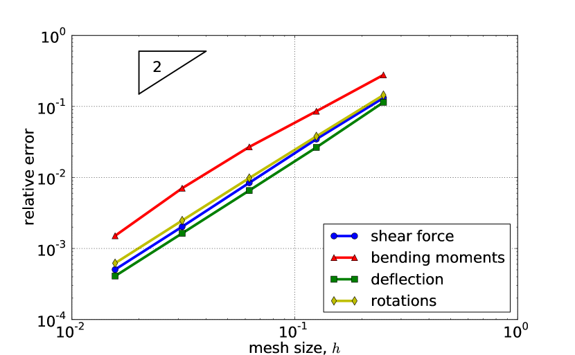
Trapezoidal

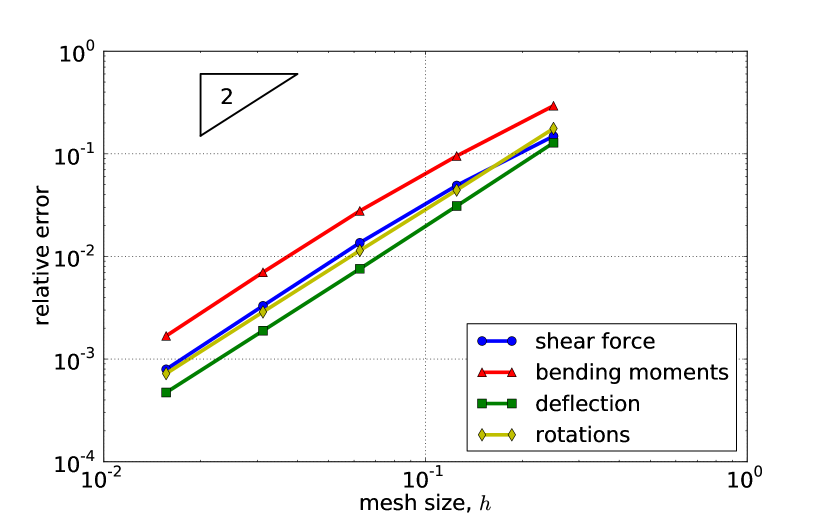
Figure 2: Convergence at $t=1/10$. Uniform versus trapezoidal mesh sequence.

Uniform

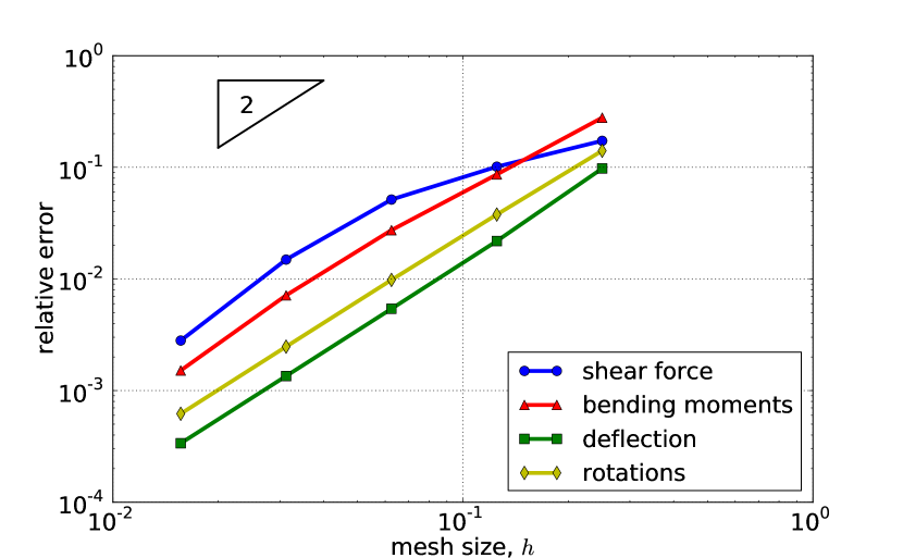
Trapezoidal

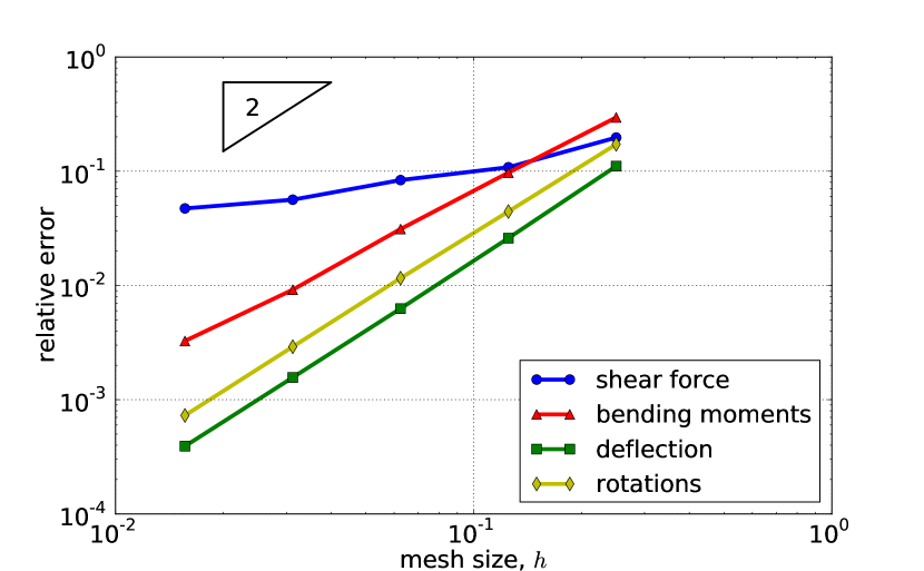
Figure 3: Convergence at $t=1/1000$. Uniform versus trapezoidal mesh sequence.

The results show that

1. Optimal quadratic convergence is attained for all quantities on both mesh sequences at $t=1/10$.

2. Convergence of the shear stress slows down at $t=1/1000$ especially on the trapezoidal mesh sequence. However, a relative error of less than 10 percent is attained also at the $16\times 16$ trapezoidal mesh.

Finally, we show in Figs. 4–7 contour plots of all quantities of interest at $t=1/1000$ obtained with DPG by using a fine mesh. The good approximation quality of all quantities makes prediction of the values and the locations of maximum stresses straightforward.

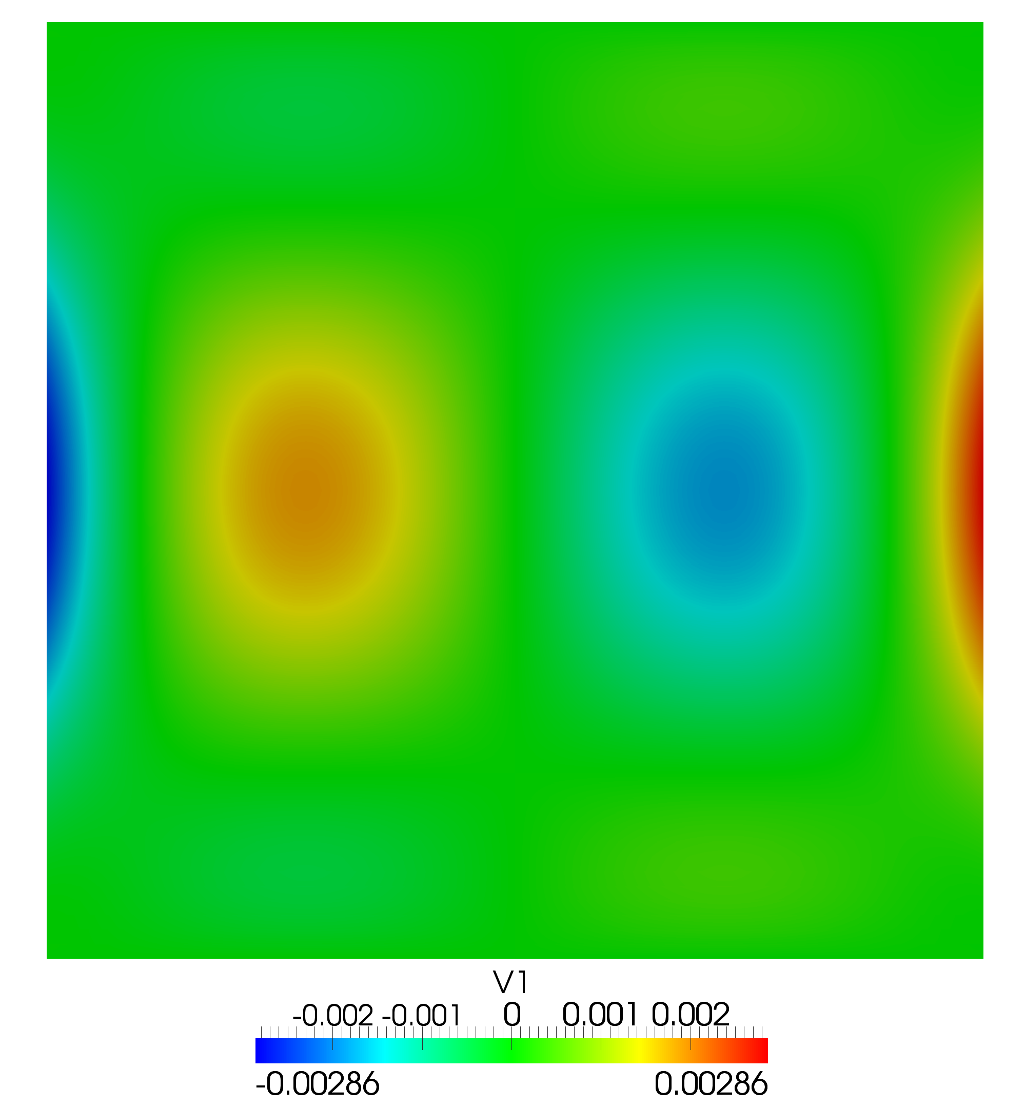
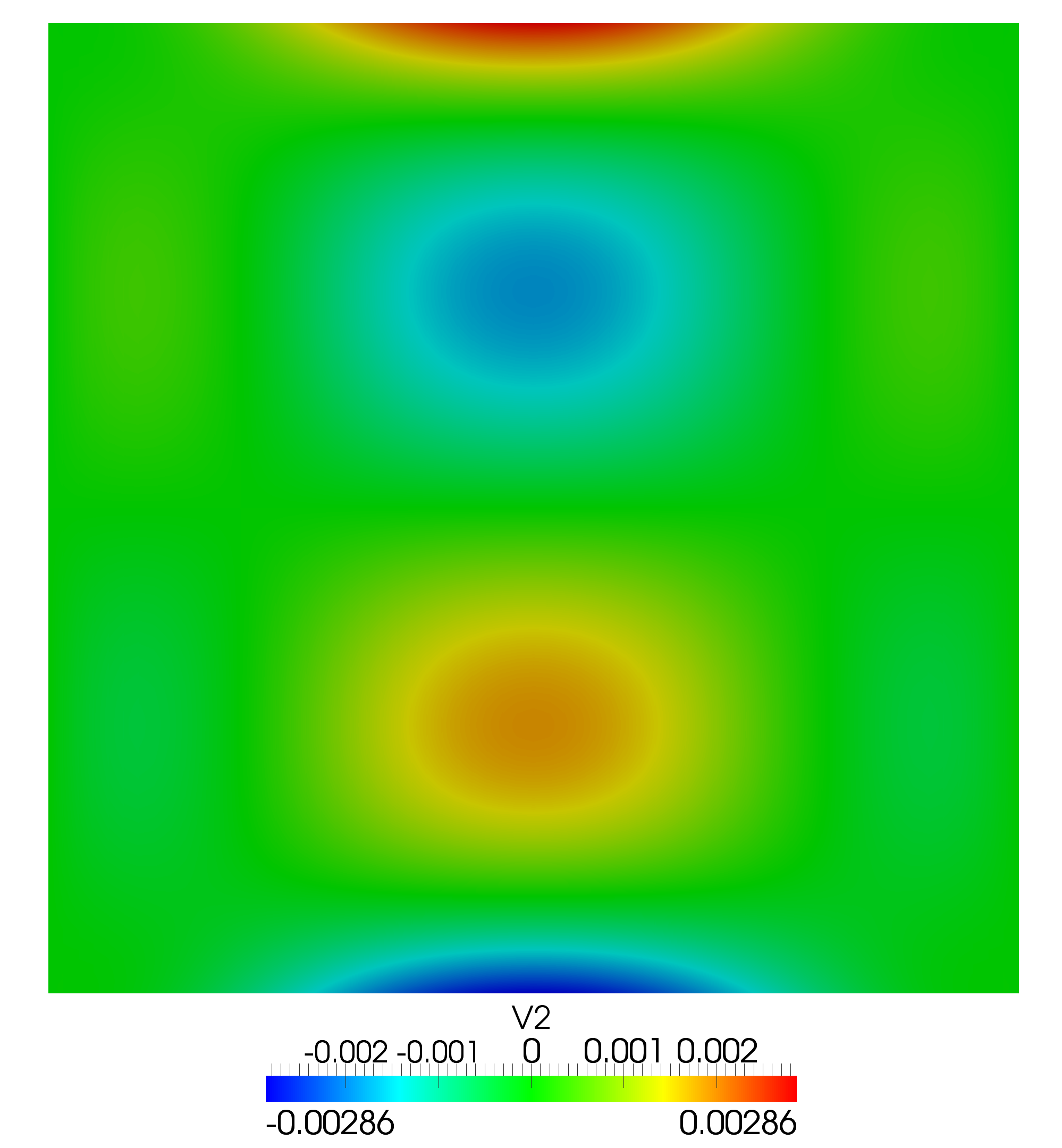
Figure 4: Shear forces at $t=1/1000$.

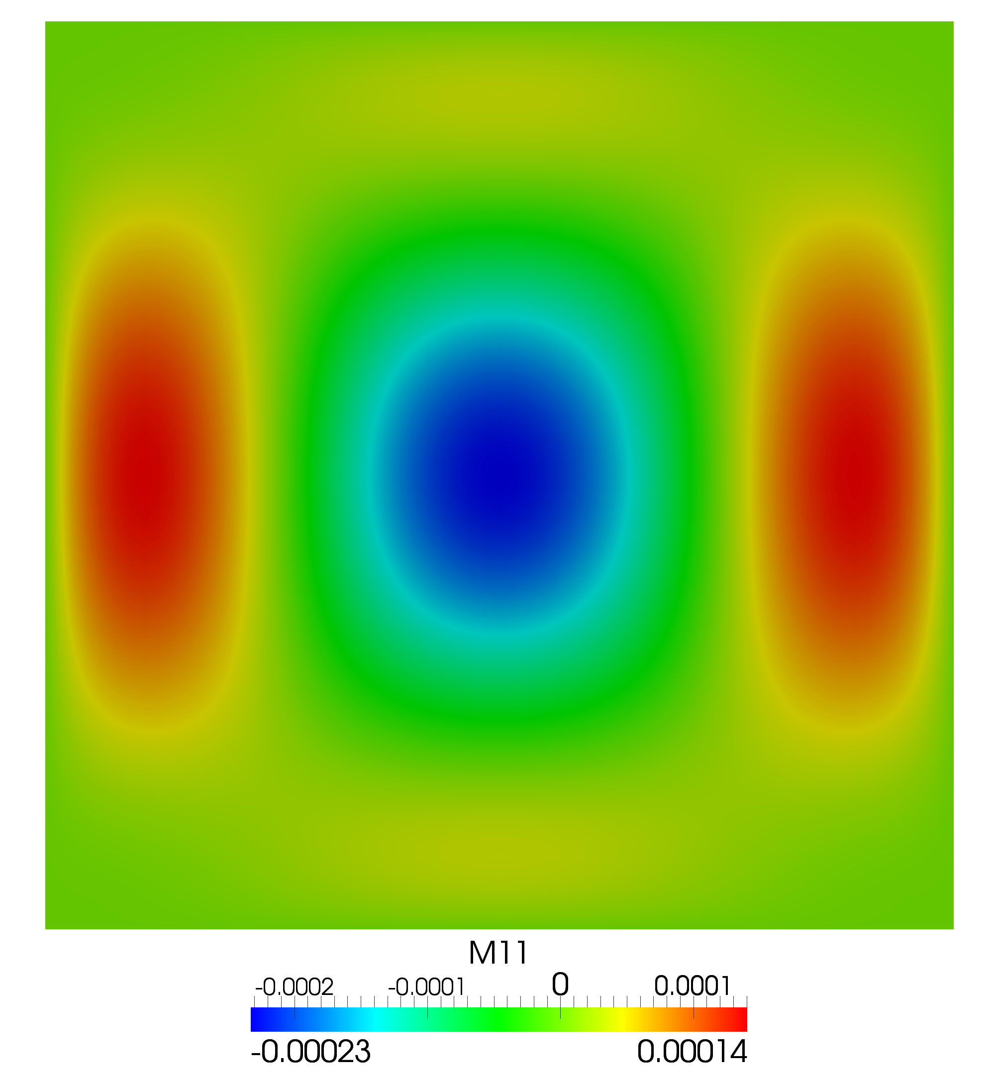
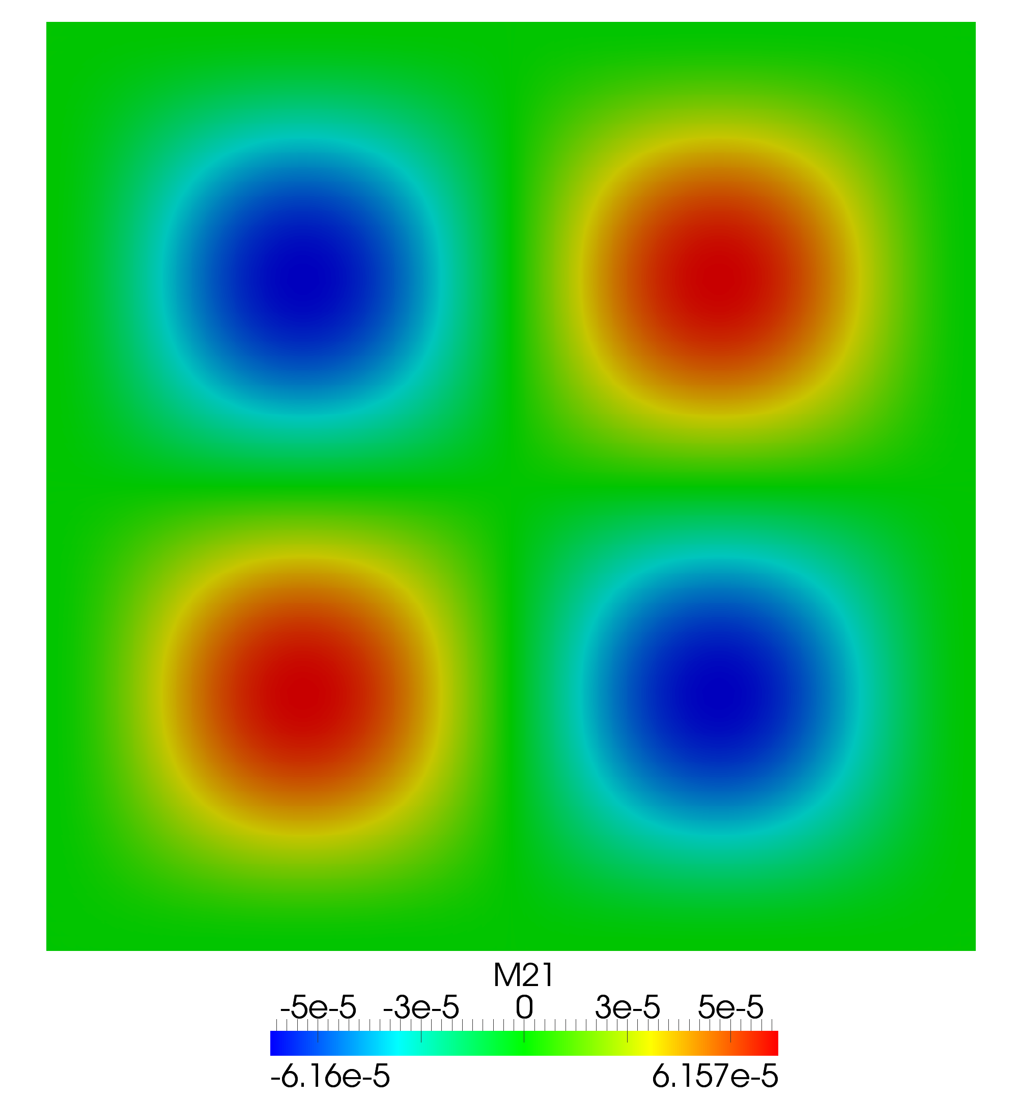
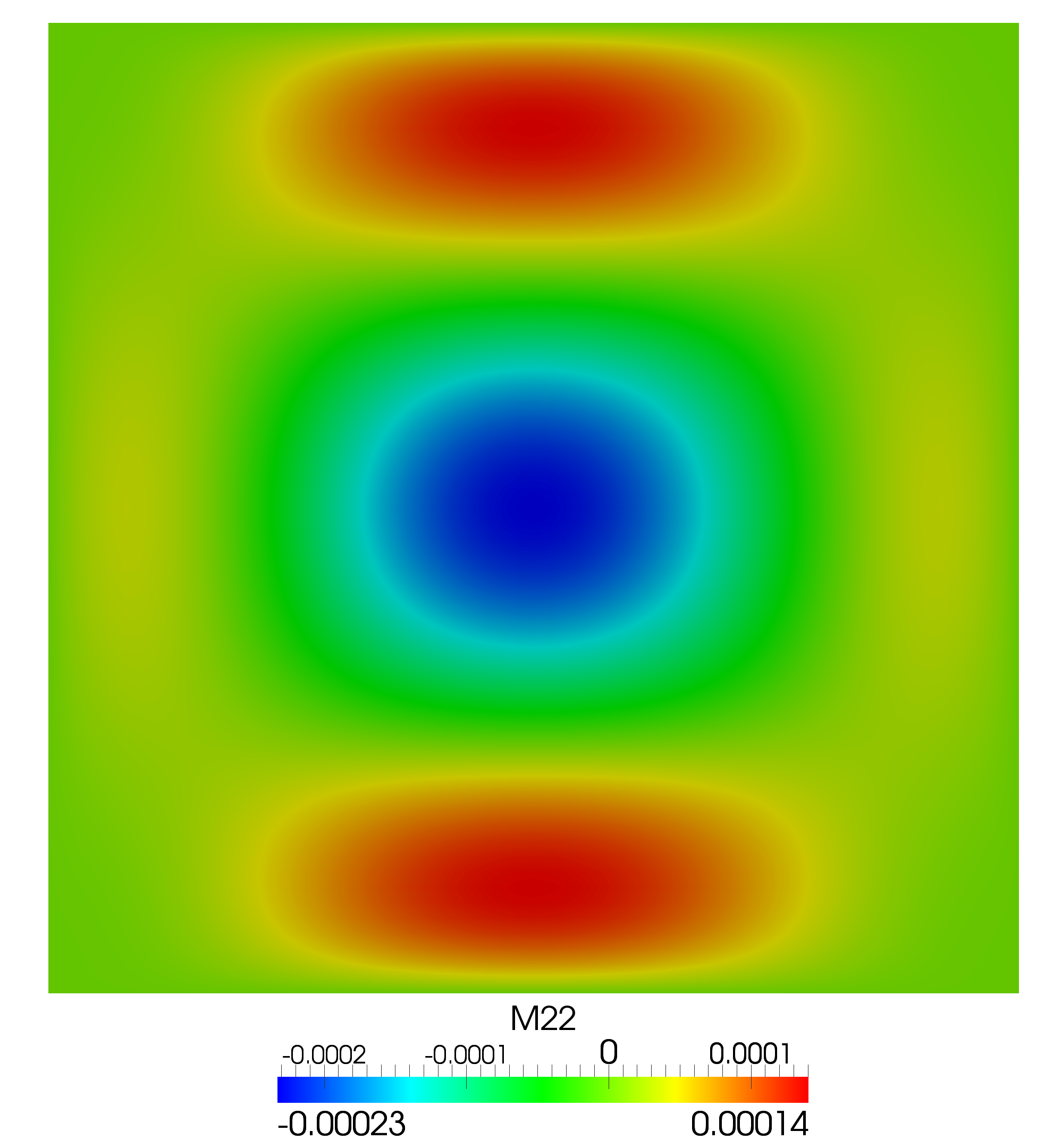
Figure 5: Bending moments at $t=1/1000$.

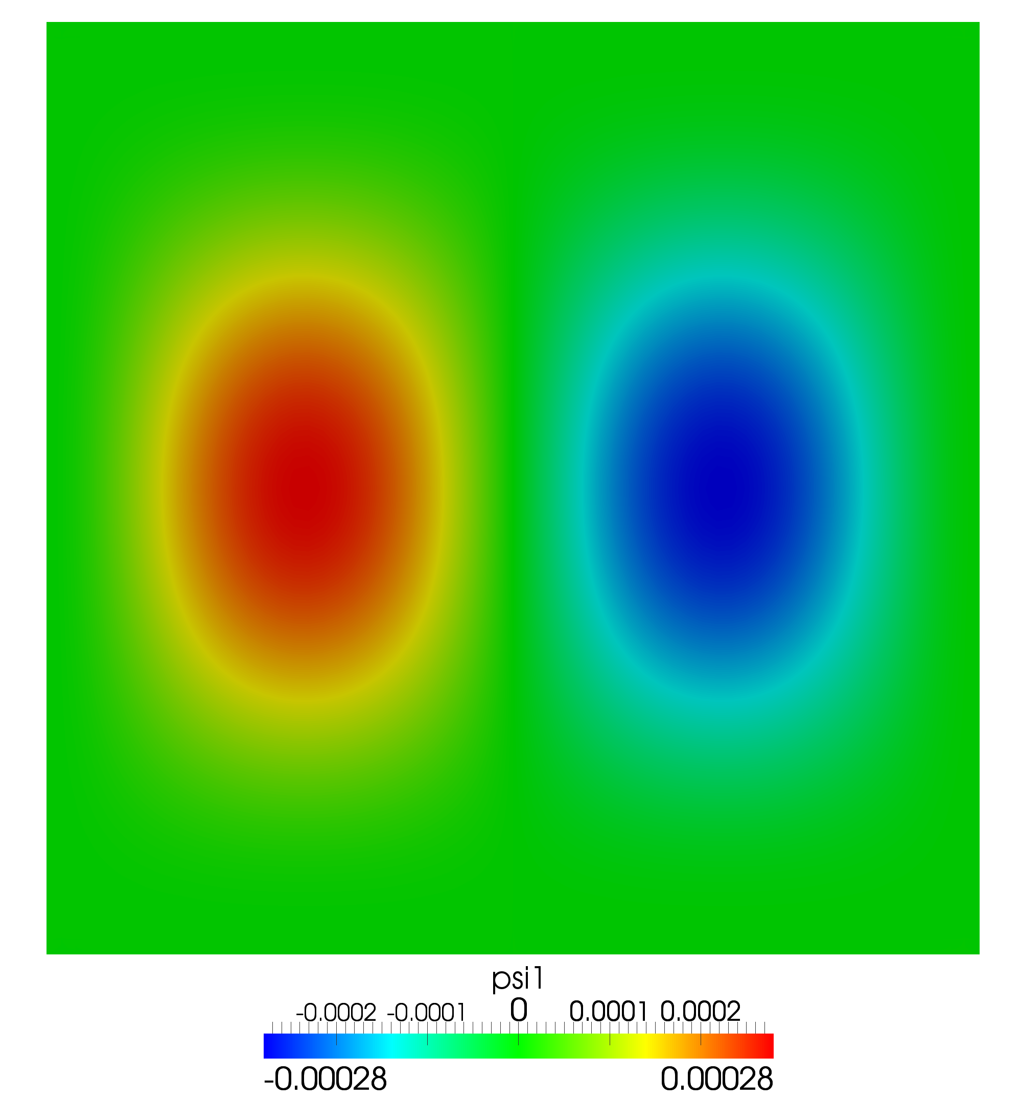
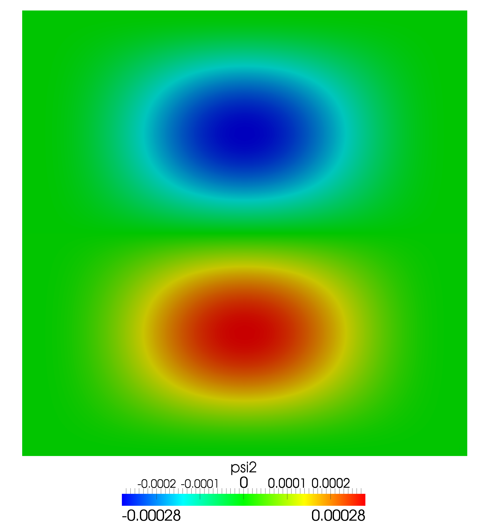
Figure 6: Rotations at $t=1/1000$.

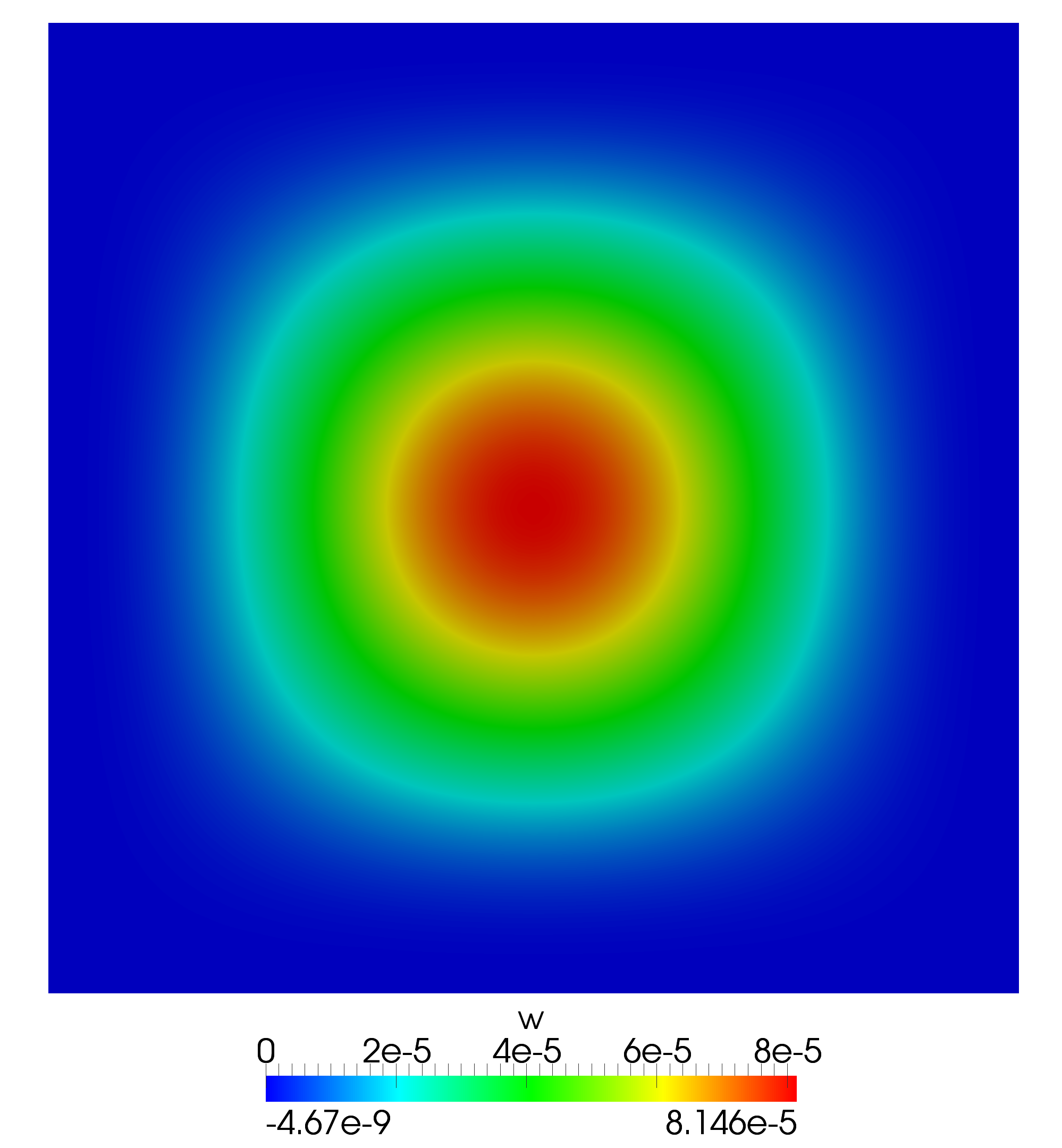
Figure 7: Transverse deflection at $t=1/1000$.

6 Concluding Remarks

We have analyzed the discontinuous Petrov-Galerkin finite element method in the Reissner-Mindlin plate bending problem. The formulation is based on a piecewise polynomial approximation using quadrilateral scalar and vector finite elements of degree $p$ for all quantities of interest (shear stress, bending moment, transverse deflection, rotation). In addition, the resultant tractions and the kinematic variables are approximated on the mesh skeleton by polynomials of degree $p$ and $p+1$, respectively.

We have showed that the non-standard variational formulation underlying the DPG method is well-posed. Based on that result, we have showed that a discretization where the test functions are approximated in an enriched finite element space of degree $p+3$ is stable as well and leads to optimal order of convergence in the $L_{2}$ norm for all variables. However, the theoretical stability estimate breaks down at the limit of zero thickness and therefore the final error bound becomes amplified by the factor $t^{-1}$. Our numerical results indicate that some error amplification indeed occurs for the shear force, but the obtained stress values are relatively accurate even on severely distorted meshes. Future work includes formulation of the algorithm for more general geometries and an evaluation of the computational cost and robustness in comparison with other type of formulations.

References

- [1] Amara, M., Capatina-Papaghiuc, D., and Chatti, A. Bending Moment Mixed Method for the Kirchhoff–Love Plate Model. SIAM Journal on Numerical Analysis 40, 5 (Jan. 2002), 1632–1649.
- [2] Arnold, D. N. Discretization by finite elements of a model parameter dependent problem. Numerische Mathematik 37, 3 (Oct. 1981), 405–421.
- [3] Arnold, D. N., Boffi, D., and Falk, R. S. Quadrilateral H (div) Finite Elements. SIAM Journal on Numerical Analysis 42, 6 (Jan. 2005), 2429–2451.
- [4] Arnold, D. N., Brezzi, F., and Marini, L. D. A Family of Discontinuous Galerkin Finite Elements for the Reissner-Mindlin Plate. Journal of Scientific Computing 22-23, 1-3 (June 2005), 25–45.
- [5] Arnold, D. N., and Falk, R. S. A Uniformly Accurate Finite Element Method for the Reissner-Mindlin Plate. SIAM Journal on Numerical Analysis 26, 6 (Dec. 1989), 1276–1290.
- [6] Babuška, I. Error-bounds for finite element method. Numerische Mathematik 16, 4 (Jan. 1971), 322–333.
- [7] Bathe, K.-J., and Dvorkin, E. N. A four-node plate bending element based on Mindlin/Reissner plate theory and a mixed interpolation. International Journal for Numerical Methods in Engineering 21, 2 (Feb. 1985), 367–383.
- [8] Behrens, E. M., and Guzmán, J. A New Family of Mixed Methods for the Reissner-Mindlin Plate Model Based on a System of First-Order Equations. Journal of Scientific Computing 49, 2 (Dec. 2010), 137–166.
- [9] Behrens, E. M., and Guzmán, J. A Mixed Method for the Biharmonic Problem Based On a System of First-Order Equations. SIAM Journal on Numerical Analysis 49, 2 (Jan. 2011), 789–817.
- [10] Beirão da Veiga, L., Mora, D., and Rodríguez, R. Numerical analysis of a locking-free mixed finite element method for a bending moment formulation of Reissner-Mindlin plate model. Numerical Methods for Partial Differential Equations (Feb. 2012).
- [11] Belytschko, T., and Tsay, C.-S. A stabilization procedure for the quadrilateral plate element with one-point quadrature. International Journal for Numerical Methods in Engineering 19, 3 (Mar. 1983), 405–419.
- [12] Braess, D. Finite elements. Theory, fast solvers, and applications in solid mechanics. Cambridge University Press, Cambridge, 2001.
- [13] Brezzi, F., Bathe, K.-J., and Fortin, M. Mixed-interpolated elements for Reissner-Mindlin plates. International Journal for Numerical Methods in Engineering 28, 8 (Aug. 1989), 1787–1801.
- [14] Chapelle, D., and Stenberg, R. An optimal low-order locking-free finite element method for Reissner-Mindlin plates. Mathematical Models and Methods in Applied Sciences (M3AS) 8, 3 (1998), 407–430.
- [15] Chinosi, C., and Lovadina, C. Numerical analysis of some mixed finite element methods for Reissner-Mindlin plates. Computational Mechanics 16, 1 (Apr. 1995), 36–44.
- [16] Chinosi, C., Lovadina, C., and Marini, L. Nonconforming locking-free finite elements for Reissner-Mindlin plates. Computer Methods in Applied Mechanics and Engineering 195, 25-28 (May 2006), 3448–3460.
- [17] Demkowicz, L., and Gopalakrishnan, J. A class of discontinuous Petrov-Galerkin methods. Part I: The transport equation. Computer Methods in Applied Mechanics and Engineering 199, 23-24 (Apr. 2010), 1558–1572.
- [18] Demkowicz, L., and Gopalakrishnan, J. A class of discontinuous Petrov-Galerkin methods. Part II: Optimal test functions. Numerical Methods for Partial Differential Equations 27 (2010), 70–105.
- [19] Demkowicz, L., and Gopalakrishnan, J. Analysis of the DPG Method for the Poisson Equation. SIAM Journal on Numerical Analysis 49, 5 (2011), 1788–1809.
- [20] Demkowicz, L., Gopalakrishnan, J., Muga, I., and Zitelli, J. Wavenumber explicit analysis of a DPG method for the multidimensional Helmholtz equation. Computer Methods in Applied Mechanics and Engineering 213-216 (Mar. 2012), 126–138.
- [21] Demkowicz, L., Gopalakrishnan, J., and Niemi, A. H. A class of discontinuous Petrov-Galerkin methods. Part III: Adaptivity. Applied Numerical Mathematics 62, 4 (Apr. 2012), 396–427.
- [22] Girault, V., and Raviart, P. A. Finite element methods for Navier-Stokes equations: theory and algorithms, vol. 5 of Springer Series in Computational Mathematics. Springer-Verlag, 1986.
- [23] Gopalakrishnan, J., and Qiu, W. An analysis of the practical DPG method. Preprint (July 2011).
- [24] Hughes, T. J. R., and Tezduyar, T. E. Finite Elements Based Upon Mindlin Plate Theory With Particular Reference to the Four-Node Bilinear Isoparametric Element. Journal of Applied Mechanics 48, 3 (1981), 587.
- [25] Macneal, R. H. A simple quadrilateral shell element. Computers & Structures 8, 2 (Apr. 1978), 175–183.
- [26] Niemi, A. H., Babuška, I., Pitkäranta, J., and Demkowicz, L. Finite element analysis of the Girkmann problem using the modern hp-version and the classical h-version. Engineering with Computers 28, 2 (June 2011), 123–134.
- [27] Niemi, A. H., Bramwell, J. A., and Demkowicz, L. F. Discontinuous Petrov-Galerkin method with optimal test functions for thin-body problems in solid mechanics. Computer Methods in Applied Mechanics and Engineering 200, 9-12 (Feb. 2011), 1291–1300.
- [28] Niemi, A. H., Collier, N. O., and Calo, V. M. Discontinuous Petrov-Galerkin method based on the optimal test space norm for steady transport problems in one space dimension. Journal of Computational Science (Aug. 2011).
- [29] Niemi, A. H., Collier, N. O., and Calo, V. M. Automatically Stable Discontinuous Petrov-Galerkin Methods for Stationary Transport Problems: Quasi-Optimal Test Space Norm. Submitted (Jan. 2012).
- [30] Pitkäranta, J. Analysis of some low-order finite element schemes for Mindlin-Reissner and Kirchhoff plates. Numerische Mathematik 53, 1-2 (Jan. 1988), 237–254.
- [31] Pitkäranta, J., and Suri, M. Design principles and error analysis for reduced-shear plate-bending finite elements. Numerische Mathematik 75, 2 (Dec. 1996), 223–266.
- [32] Pitkäranta, J., and Suri, M. Upper and lower error bounds for plate-bending finite elements. Numerische Mathematik 84, 4 (Feb. 2000), 611–648.
- [33] Szabó, B. A., Babuška, I., Pitkäranta, J., and Nervi, S. The problem of verification with reference to the Girkmann problem. Engineering with Computers 26, 2 (Nov. 2009), 171–183.
- [34] Ventsel, E., and Krauthammer, T. Thin Plates and Shells. CRC Press, 2001.
- [35] Zitelli, J., Muga, I., Demkowicz, L., Gopalakrishnan, J., Pardo, D., and Calo, V. M. A class of discontinuous Petrov-Galerkin methods. Part IV: The optimal test norm and time-harmonic wave propagation in 1D. Journal of Computational Physics 230 (2011), 2406–2432.