Nonlocal actin orientation models select for a unique orientation pattern.

Abstract

Many models have been developed to study the role of branching actin networks in motility. One important component of those models is the distribution of filament orientations relative to the cell membrane. Two mean-field models previously proposed are generalized and analyzed. In particular, we find that both models uniquely select for a dominant orientation pattern. In the linear case, the pattern is the eigenfunction associated with the principal eigenvalue. In the nonlinear case, we show there exists a unique equilibrium and that the equilibrium is locally stable. Approximate techniques are then used to provide evidence for global stability.

1 Introduction

Actin is a protein involved in many cellular processes ranging from regulating gene transcription to acting as a motor in cell motility [9]. It is one of the most conserved proteins and is present in almost all eukaryotic cells. Actin monomers polymerize into thin filaments which form highly branched networks near the leading edge of motile cells [19]. While actin monomers will spontaneously polymerize in physiological conditions, inside these branched networks, new filaments are generated by branching off of existing filaments [23]. New filaments are nucleated by the actin related proteins 2 and 3 complex (Arp2/3). To maintain a consistent supply of actin monomers, actin filaments are eventually severed and depolymerized. Filament density is regulated by capping protein binding to the filament tips, ceasing polymerization [7]. Combined with filaments growing by the addition of new monomers, these processes create a dynamic network that serves as the engine in certain types of cell motility [23, 25].

Any individual filament in an actin network can be partially characterized by the angle between it and the normal direction of the membrane. One obvious question is whether or not these angles form any regular pattern. While the question has not been extensively studied experimentally, there is some evidence that the networks indeed organize into regular patterns relative to the cell membrane [15, 32, 26, 30]. A few models have been proposed to explain the existence of such patterns [15, 28, 31]. While these models have been numerically studied, there has been no rigorous work proving the existence, uniqueness or stability of these solutions. This article presents a few results that characterize the solutions to two equations modeling the angular density of branching actin networks.

All of the models proposed to explain the orientation distribution have used a continuum approximation. There is some question as to whether or not ignoring the stochastic fluctuations of actin networks is justified [25]. However, none of the models make specific predictions about the kinetics of network organization, and there is currently no evidence that correlations between filaments lead to changes in the equilibrium orientation pattern. For the rest of this article, we will assume the approximation is justified and focus on long-time equilibrium behavior.

Some of the first few models to study orientation patterns in actin and similar networks studied the existence and persistence of peaks in the orientation pattern [12, 17, 16]. The analysis was based on Fourier series and small perturbations which greatly limited their generality. Their analysis led to the qualitative result that peaked orientation patterns are likely to be observed. Similar methods have been used on models of orientation and space [11, 5]. Stability analysis has also been done on similar models, termed “ring models” in the neuroscience literature [4, 33].

The first model we consider here was proposed by Maly and Borisy [15]. Their insight was that if filaments were capped at different rates based on the filament orientation, filament branching and capping could generate stable orientation patterns. The model they proposed takes into account branching and capping explicitly and filament growth implicitly. New filaments branch off of existing filaments at a characteristic angle $\sim 70^{\circ}$ with some variance around that. We can write out a branching kernel as a probability of a mother filament with angle $\theta_{M}$ having a branched daughter filament with angle $\theta_{D}$:

$$\mathcal{B}(\phi)=\mathrm{P}(\theta_{D}=\theta_{M}-\phi)$$ (1)

Adding up the contribution of all filaments with density $u(\phi)$ gives the total branching rate at angle $\theta$:

$$\text{BR}(\theta)\propto\int\mathcal{B}(\theta-\phi)u(\phi)\,\mathrm{d}\phi$$ (2)

They also proposed that the capping rate was proportional to the amount of time the filament would be not in contact with the leading edge, much like [18], but used the capping function $\frac{1}{\cos(\theta)}$. The Maly and Borisy model only considered filaments growing faster than the leading edge, i.e. filaments with orientation $|\theta|\leq\theta_{\text{crit}}=\arccos\left[\frac{v}{v_{max}}\right]$ where $\frac{v}{v_{max}}$ is the velocity of the leading edge relative to the maximum velocity of filament growth. Combining the two terms gives the full equation:

$$\dot{u}(\theta,t)=\lambda\int\limits_{-\theta_{\text{crit}}}^{\theta_{\text{crit}}}\mathcal{B}(\theta-\phi)u(\phi)\,\mathrm{d}\phi-\frac{u(\theta,t)}{\cos(\theta)}$$ (3)

where $\dot{u}$ indicates the time derivative. The equation is defined on $(-\theta_{\text{crit}},\theta_{\text{crit}})\times\mathbb{R}^{+}$ with absorbing boundary conditions.

Maly and Borisy performed two analyses on (3). The first analysis was to approixmate solutions of (3) by solving the equation for two points in orientation space. Solutions to the two-point approximation supported the argument that the equation selected for a unique orientation ‘type’ that grew exponentially at the fastest rate. The second analysis was to use numerical quadrature [3] to approximate the eigenfunctions of the right-hand side of (3). However, the existence and uniqueness of the eigenfunction solutions were never rigorously shown. They explained their results by using an evolutionary selection metaphor. In this article, we show that a version of (3) with stricter hypotheses on the capping rate uniquely selects for a most ’fit’ orientation pattern with a fitness function defined on the unit ball of orientation functions.

A very similar model was proposed by Weichsel and Schwartz [31] to explain both the orientation patterns and the velocity of a growing actin network pushing against a given force. There were two primary differences between their model and the Maly and Borisy model. First, orientations were defined on the entire circle, $S^{1}$. The second difference was to normalize the total branching rate to the constant $\lambda$, which ensures that solutions have bounded total density. The Weichsel and Schwartz model is:

$$\dot{u}(\theta,t)=\frac{\lambda}{\int_{S^{1}}u(\phi,t)\,\mathrm{d}\phi}\int\limits_{S^{1}}\mathcal{B}(\theta-\phi)u(\phi,t)\,\mathrm{d}\phi-\kappa(\theta)u(\theta,t)$$ (4)

where the capping rate is a constant plus a term proportional to the difference between the velocity of the leading edge and a filament with a given orientation:

$$\kappa(\theta)=k+c\left(v_{LE}-v_{0}\cos(\theta)\right)^{+}$$ (5)

where $v_{LE}$ is the velocity of the leading edge, $v_{0}$ is the rate of filament growth, and $(x)^{+}$ is the positive part of $x$.

Weichsel and Schwartz performed the same two analyses as in the Maly and Borisy paper. They found that, for certain parameters, there were two equilibria in the two-point approximation to (4), where one equilibrium is stable and the other is a saddle. Finally, they used numerical techniques to calculate the equilibrium distributions. The results in this article explicitly contradict their assertion of multiple equilibria, but they show the local stability of a unique, positive equilibrium. However, it is important to note that the equilibrium is unique for a fixed $\mathcal{B}$ and $\kappa$. Changing the load force, concentrations of branching and capping proteins, or other experimental manipulations could change the structure of the unique equilibrium.

The core tool used in this paper to prove the existence and uniqueness of a principal eigenvalue is the Krein-Rutman theorem. The theorem is one of the key tools in studying transfer and diffusion operators with applications in biology [22], physics [10], and materials science [6]. The work presented here is relatively novel in that we show the equivalence of the spectrum between our operator of interest and a positive operator before using the Krein-Rutman theorem on the positive operator.

1.1 Definitions and Assumptions

The two equations we specifically analyze are:

$$\dot{u}(\theta,t) =\lambda\Big{(}\mathcal{B}\star u\Big{)}(\theta,t)-\kappa(\theta)u(\theta,t)$$ (6)

$$\dot{u}(\theta,t) =\frac{b}{\int u(\omega,t)\,\mathrm{d}\omega}\Big{(}\mathcal{B}\star u\Big{)}(\theta,t)-\kappa(\theta)u(\theta,t)$$ (7)

Equation 6 is our generalization of the Maly and Borisy [15] model, and equation 7 is our generalization of the Weichsel and Schwarz [31] model. Both equations are defined on the circle $S^{1}$ with $\mathcal{B}\geq 0$ being the branching kernel which generates new filaments and $\kappa(\theta)>0$ being the variable capping rate which eliminates filaments. The hypotheses on each function are relatively weak:

1. $\mathcal{B}$ is real, positive, symmetric $C^{2}$ function with $\|B\|_{1}=1$.

2. $\kappa$ is a real, strictly positive, symmetric $C^{2}$ function

The assumptions are likely stronger than necessary, but generalizing the problem is a question for further study. They also do not exactly capture the dynamics for either paper. The first paper, by Maly and Borisy [15], would require an infinite capping rate. However, as that is likely unphysical, the equations at hand should be sufficient. For Weichsel and Schwarz [31], the capping rate they used is continuous but not differentiable. The primary role of the $C^{2}$ hypothesis on $\mathcal{B}$ is to ensure compactness, and weaker hypotheses should be quite feasible. Likewise, the $C^{2}$ hypothesis is stronger than necessary, but it simplifies the presentation. The smoothness hypotheses are merely technical and should have no effect on the interpretation of the results presented here.

In agreement with the paper [15], the first-order branching equation uniquely selects for an optimal orientation pattern. However, the Weichsel and Schwarz paper [31] suggests that there might be multiple equilibria. We show that the zeroth-order branching equation also uniquely selects for a unique equilibrium orientation pattern.

The first two results characterize solutions to the first-order branching equation (6). Theorem 2 shows that the spectrum of the operator defining (6) is dominated by an isolated, simple principal eigenvalue with strictly positive eigenfunction. While that eigenvalue may be positive or negative in general, long-time solutions to (6) are therefore dominated by the exponential increase or decay of the principal eigenfunction. Proposition 8 says that for given $\mathcal{B}$ and $\kappa$, there exists only one $\lambda$ such that (6) has a non-trivial equilibrium.

The rest of the article is dedicated to analyzing (7). Proposition 13 gives the existence and uniqueness of a non-trivial equilibrium. Linear stability analysis combined with Theorem 15 implies that the equilibrium is locally stable. Finally, numerical simulations and a perturbation analysis are performed to provide evidence that (7) is globally stable.

2 First-order Branching

The first result uniquely characterizes the dynamics of (6). Define $\mathrm{A}$ to be the linear operator on the right-hand side of (6):

$$\mathrm{A}=\lambda\Big{(}\mathcal{B}\star u\Big{)}(\theta,t)-\kappa(\theta)u(\theta,t)$$ (8)

For the sake of brevity, we will forego much discussion of the existence and uniqueness of solutions to equation (6). It is known that a densely-defined resolvent positive operator fulfills the Hille-Yosida conditions, which ensures unique, positive solutions [1]. We will sketch a quick lemma showing that $\mathrm{A}$ is resolvent positive as it is illustrative of future techniques:

Lemma 1.

$\mathrm{A}$ is a resolvent positive operator, i.e. there exists $\gamma_{0}\in\mathbb{R}$ such that for all $\gamma\in\mathbb{R}$ where $\gamma>\gamma_{0}$:

$$(\gamma-\mathrm{A})^{-1}\geq 0$$ (9)

Proof.

For the sake of this sketch, we will avoid the details regarding the underlying space $A$ is defined on and will define inequalities pointwise. Choose $\gamma_{0}=\rho(\mathrm{A})$. Fix $\gamma\in\mathbb{R}$ where $\gamma>\gamma_{0}$ and some positive function $f\geq 0$. It suffices to show that $g\geq 0$ where $g$ is:

$$(\gamma-\mathrm{A})^{-1}f=g$$ (10)

Working things out, we can observe:

$$(\gamma-\mathrm{A})^{-1}f =g \iff$$

$$f =(\gamma-\mathrm{A})g \iff$$

$$f =(\gamma+\kappa)g-\mathcal{B}\star g \iff$$

$$\frac{f}{\gamma+\kappa} =g-\frac{\mathcal{B}\star g}{\gamma+\kappa}$$

Define $\mathrm{B}_{\gamma}=\frac{\mathcal{B}\star}{\gamma+\kappa}$. We can now use the Neumann series to finish the proof:

$$g =(1-\mathrm{B}_{\gamma})^{-1}f \iff$$

$$g =\sum_{k=0}^{\infty}B_{\gamma}^{k}f\geq 0$$ (11)

The last inequality comes from our hypothesis that $\mathcal{B}\geq 0$. ∎

The main result we are showing here is as follows:

Theorem 2.

$\mathrm{A}$ has an isolated, algebraically simple principal eigenvalue with positive eigenfunction.

To make things more readable, we will break the proof out into a number of lemmas and combine them at the end. Much of the analysis in this section relies on proving facts for $\mathrm{A}$ as an operator on the space $\mathnormal{L}^{2}$ and generalizing to $\mathnormal{L}^{1}$. Before doing so, a quick lemma to ensure $\mathrm{A}$ is bounded on both spaces.

Lemma 3.

$\mathrm{A}$ is a bounded linear operator on both $\mathnormal{L}^{1}$ and $\mathnormal{L}^{2}$.

Proof.

By the hypothesis that $\mathcal{B}$ is bounded, we use Young’s inequality to observe:

$$\|\mathcal{B}\star u\|_{1} \leq\|\mathcal{B}\|_{\infty}\|u\|_{1}$$

$$\|\mathcal{B}\star u\|_{2} \leq\|\mathcal{B}\|_{2}\|u\|_{2}$$ (12)

The convolution is therefore a bounded operator on both spaces. Since $\mathrm{A}$ is the sum of the convolution and multiplication by a bounded function, we can conclude that $\mathrm{A}$ is a bounded operator ∎

A fact about $\mathcal{B}\star\cdot$ we need:

Lemma 4.

The operator $(\mathcal{B}\star u)(\theta)$ is compact.

Proof.

When we are considering the operator $\mathcal{B}\star\cdot$ over $\mathnormal{L}^{2}$, we can simply observe that $\mathcal{B}(\theta-\omega)$ is a Hilbert-Schmidt kernel and that implies that the convolution is compact. However, proving compactness over $\mathnormal{L}^{1}$ is slightly more difficult. We will use the Arzelà-Ascoli theorem to show that $\mathcal{B}\star\cdot$ maps bounded sequences to sequences with a convergent subsequence.

Take a sequence of functions $\{f_{n}\}_{n\in\mathbb{N}}$ where $\|f_{n}\|_{1}\leq 1$. Using Young’s inequality as above, we obtain a uniform bound on $\|\mathcal{B}\star f_{n}\|_{\infty}$:

$$\|\mathcal{B}\star f_{n}\|_{\infty}\leq\|\mathcal{B}\|_{\infty}\|f_{n}\|_{1}\leq\|B\|_{\infty}$$ (13)

Since $\mathcal{B}\in C^{2}$, we know that $\|\mathcal{B}^{\prime}\|_{\infty}<\infty$. We can again apply Young’s inequality to show that the derivative of $\mathcal{B}\star f_{n}$ is uniformly bounded:

$$\|(\mathcal{B}\star f_{n})^{\prime}\|_{\infty}=\|\mathcal{B}^{\prime}\star f_{n}\|_{\infty}\leq\|\mathcal{B}^{\prime}\|_{\infty}\|f_{n}\|_{1}\leq\|B^{\prime}\|_{\infty}$$ (14)

The $(\mathcal{B}\star f_{n})^{\prime}$ being uniformly bounded implies that $\{\mathcal{B}\star f_{n}\}$ is uniformly Lipschitz. That means that Arzelà-Ascoli holds and $\mathcal{B}\star\cdot$ is compact. ∎

Here, we should introduce a bit of notation to clarify which space we are considering when we talk about the spectrum of $\mathrm{A}$. $\sigma_{1}(\mathrm{A})$ refers to the spectrum of $\mathrm{A}$ over the space $\mathnormal{L}^{1}$, and $\sigma_{2}(\mathrm{A})$ is the spectrum over $\mathnormal{L}^{2}$. We can now state and prove a lemma which characterizes the spectrum of $\mathrm{A}$ for much of the complex plane.

Lemma 5.

All elements of $\sigma_{1}(\mathrm{A})$ and $\sigma_{2}(\mathrm{A})$ outside of the line $-R(\kappa)=[-\sup\kappa,-\inf\kappa]$ are eigenvalues.

Proof.

This result holds equally for all the $\mathnormal{L}^{p}$ spaces. I will prove the result for $\mathnormal{L}^{1}$. The argument holds by simply replacing the metric $\|\cdot\|_{1}$ with $\|\cdot\|_{p}$. The eigenfunctions over $\mathnormal{L}^{1}$ are bounded, so are in all of the $\mathnormal{L}^{p}$ spaces. Fix a number $\mu\in\sigma_{1}(\mathrm{A})$ with $\mu\notin[-\sup\kappa,-\inf\kappa]$ and in either the continuous spectrum or the point spectrum. Since $\mu$ is not in the residual spectrum, we have a sequence $\{u_{n}\}_{n\in\mathbb{N}}\subset\mathnormal{L}^{1}$ with $\|u_{n}\|_{1}$ such that:

$$\lim_{n\rightarrow\infty}\|(\mathrm{A}-\mu\mathrm{I})u_{n}\|_{1}=0$$

By invoking the compactness of $\mathcal{B}\star\cdot$ from the previous step, there exists a subsequence $u_{n_{k}}$ such that:

$$0=\lim_{k\to\infty}\|(\mathrm{A}-\mu\mathrm{I})u_{n_{k}}\|_{1} =\lim_{k\to\infty}\|(\mathcal{B}\star u_{n_{k}})(\theta)-(\kappa(\theta)+\mu)u_{n_{k}}(\theta)\|_{1}$$

$$=\lim_{k\to\infty}\|v(\theta)-(\kappa(\theta)+\mu)u_{n_{k}}(\theta)\|_{1}$$

where $v$ is the limit of $\mathcal{B}\star u_{n_{k}}$. By hypothesis, $\kappa(\theta)+\mu\neq 0$, so $\displaystyle\frac{1}{\kappa(\theta)+\mu}$ is bounded. We now have that:

$$\lim_{k\to\infty}u_{n_{k}}(\theta)=\frac{v(\theta)}{\kappa(\theta)+\mu}=w(\theta)$$

almost everywhere. By the fact that $\mathcal{B}\star\cdot$ is closed, $(\mathcal{B}\star w)(\theta)=v(\theta)$. Applying the above identities shows that $\mathrm{A}w=\mu w$. Finally, observe that $w\in\mathnormal{L}^{\infty}$ since:

$$w=\frac{\mathcal{B}\star w}{\kappa+\mu}$$ (15)

$\mathcal{B}\star w$ is bounded by Young’s inequality and $\displaystyle\frac{1}{\kappa(\theta)+\mu}$ is bounded by hypothesis. ∎

We can show an even stronger correspondence between $\sigma_{1}(\mathrm{A})$ and $\sigma_{2}(\mathrm{A})$.

Lemma 6.

The spectra $\sigma_{1}(\mathrm{A})$ and $\sigma_{2}(\mathrm{A})$ are equal outside of $[-\sup\kappa,-\inf\kappa]$.

Proof.

To show this, we will consider the spectrum in three parts, the point spectrum, the continuous spectrum, and the residual spectrum. Any eigenvalue of $\mathrm{A}$ on $\mathnormal{L}^{2}$ is an eigenvalue on $\mathnormal{L}^{1}$ by the inclusion $\mathnormal{L}^{2}\subset\mathnormal{L}^{1}$. The reverse inclusion comes from the fact that all of the eigenvalues over $\mathnormal{L}^{1}$ outside of $[-\sup\kappa,-\inf\kappa]$ are in $\mathnormal{L}^{\infty}\supset\mathnormal{L}^{2}$. We now have that the two point spectrums are equal. The result in step 3 implies that there is no elements of the continuous spectrum outside of $[-\sup\kappa,-\inf\kappa]$, which implies the continuous spectrums are equal. All that remains is to show that $\mathrm{A}$ has no residual spectrum on either $\mathnormal{L}^{2}$ or $\mathnormal{L}^{1}$.

The natural embedding of $\mathnormal{L}^{q}$ into $\mathnormal{L}^{p}$ where $1\leq p<q\leq\infty$ is a dense embedding. Continuous functions are dense in $\mathnormal{L}^{1}$ as can be seen by approximating simple functions by continuous functions. Since continuous functions are in $\mathnormal{L}^{\infty}$, that implies $\mathnormal{L}^{\infty}$ is dense in $\mathnormal{L}^{1}$. By the inclusion $\mathnormal{L}^{q}\subset\mathnormal{L}^{1}$, continuous functions are dense in $\mathnormal{L}^{q}$ for all $1<q\leq\infty$.

The last step remains to show that $\mathrm{A}$ has no residual spectrum over neither $\mathnormal{L}^{2}$ nor $\mathnormal{L}^{1}$. By self-adjointness, $\mathrm{A}$ has no residual spectrum over $\mathnormal{L}^{2}$. The fact that $\mathrm{A}$ has no residual spectrum over $\mathnormal{L}^{1}$ follows immediately from the density of the embedding $\mathnormal{L}^{2}$ in $\mathnormal{L}^{1}$. We know that $\mathrm{A}-\mu\mathrm{I}$ has dense range in $\mathnormal{L}^{2}$ for all $\mu\in\mathbb{C}$ whenever $\mu$ is not an eigenvalue. Assume $\mu$ is not an eigenvalue, the dense embedding and $\mathrm{A}-\mu\mathrm{I}$ having dense range in $\mathnormal{L}^{2}$ implies that $\mathrm{A}-\mu\mathrm{I}\Big{|}_{\mathnormal{L}^{2}}$ is dense in $\mathnormal{L}^{1}$. That implies that $\mathrm{A}-\mu\mathrm{I}\Big{|}_{\mathnormal{L}^{1}}$ is dense in $\mathnormal{L}^{1}$ and that $\mu$ is not in the residual spectrum. ∎

Moving away from the operator theory world for a moment, we need a more set theoretic lemma for proving that the principal eigenvalue is simple.

Lemma 7.

For any given kernel $\mathcal{B}$, there exists $n$ such that $\Big{(}\mathrm{B}_{\gamma}\Big{)}^{n}$ is strongly positive, i.e.:

$$u\geq 0\implies\Big{(}\mathrm{B}_{\gamma}\Big{)}^{n}u>0$$

whenever $u\geq 0$ is a continuous function not uniformly zero and $\gamma>-\inf\kappa$.

Proof.

We are only concerned with whether or not $\Big{(}\mathrm{B}_{\gamma}\Big{)}^{n}$ is positive and not on the specific value of $\Big{(}\mathrm{B}_{\gamma}\Big{)}^{n}$, so it is sufficient to show the result for $\mathrm{B}^{n}$ where $\mathrm{B}u=\mathcal{B}\star u$. Define $\Sigma$ to be the $\sigma-$algebra associated with the Lebesgue measure on $S^{1}$. We can define the set mapping $T:\Sigma\to\Sigma$ as:

$$T\Omega=\mathop{\operator@font supp}\nolimits\{\mathcal{B}\star\mathbf{1}_{\Omega}\}$$ (16)

where $\Omega\in\Sigma$. Choose some open interval $(y-\delta,y+\delta)\subset\mathop{\operator@font supp}\nolimits\{\mathcal{B}\}$ for $y\neq 0$, $y\in\mathbb{R}\backslash\mathbb{Q}$. Assume $\Omega$ contains an open interval $(x-\varepsilon,x+\varepsilon)$. Observe that for every $z\in(x+y-\delta,x+y+\delta)$:

$$\mathcal{B}\star\mathbf{1}_{\Omega}(z)=\int\mathcal{B}(z-s)\mathbf{1}_{\Omega}(s)\,\mathrm{d}s\geq\int\limits_{x-\varepsilon}^{x+\varepsilon}\mathcal{B}(z-s)\,\mathrm{d}s=\int\limits_{y-\varepsilon}^{y+\varepsilon}\mathcal{B}\Big{(}(z-x+y)-s^{\prime}\Big{)}\,\mathrm{d}s^{\prime}>0$$ (17)

The above argument also holds for $z\in(x-y-\delta,x-y+\delta)$. Notice that while the existence of the interval was used in the above calculation, there is no explicit dependence on $\varepsilon$ beyond that $\varepsilon>0$. Iterating $T$, we can observe that:

$$T^{2n}\Omega\subset\cup_{0\leq j\leq n}\Big{(}(x+2jy-\delta,x+2jy+\delta)\cup(x-2jy-\delta,x-2jy+\delta)\Big{)}$$ (18)

By the fact that $x+2y$ is an irrational rotation, $\{x+2jy\}_{j\in\mathbb{N}}$ is dense in $S^{1}$ and the sets $\{(x+2jy-\delta,x+2jy+\delta)\}_{j\in\mathbb{N}}$ form an open covering of $S^{1}$. The compactness of $S^{1}$ implies that there exists $n\in\mathbb{N}$ such that $S^{1}\subset\cup_{1\leq j\leq n}(x+2jy-\delta,x+2jy+\delta)$. Rotational symmetry in $S^{1}$ implies that $n$ has no dependence on $x$. Fix some function $u\in C(S^{1})$ with $u\geq 0$ and $u$ not uniformly zero. We can set $\Omega=\mathop{\operator@font supp}\nolimits\{u\}$ and observe $\Omega$ contains an open interval containing some $x^{\prime}$. The above discussion implies:

$$T^{2n}\Omega\supset\cup_{1\leq j\leq n}(x^{\prime}+2jy-\delta,x^{\prime}+2jy+\delta)\supset S^{1}$$ (19)

The above set relation implies $\mathrm{B}^{2n}u>0$. ∎

We can now show the main result of this section, Theorem 2.

Proof.

Since $\mathrm{A}$ is self-adjoint, we know the spectrum over $\mathnormal{L}^{2}$ is bounded by the eigenvalue $\mu_{0}$:

$$\mu_{0}=\sup_{\|u\|_{2}=1}\langle\mathrm{A}u,u\rangle$$ (20)

By lemma 5, we know that $\mu_{0}$ is an eigenvalue as long as $\mu_{0}>-\inf\kappa$. It suffices to show there exists $u\in\mathnormal{L}^{2}$ such that:

$$\langle\mathrm{A}u,u,\rangle+\inf\kappa\langle u,u\rangle>0$$ (21)

By the continuity of $\kappa$ and compactness of the circle, $\kappa(\theta)-\inf\kappa=0$ for at least one $\theta$. For the sake of notation, define $g(\theta)=\kappa(\theta)-\inf\kappa$.

Observe that for any function of the form $u(\theta)=c+f(\theta)\geq 0$ with $c,\,f(\theta)\geq 0$ where $\int_{S^{1}}u(\theta)=1$:

$$\langle\mathcal{B}\star u,u\rangle =\iint\limits_{S^{1}S^{1}}\mathcal{B}(\theta-\omega)(c+f(\omega))\,\mathrm{d}\omega(c+f(\theta))\,\mathrm{d}\theta$$

$$\geq c\iint\limits_{S^{1}S^{1}}\mathcal{B}(\theta-\omega)(c+f(\theta))\,\mathrm{d}\omega\,\mathrm{d}\theta=c$$

since $f(\theta)\geq 0$ and $\int\mathcal{B}=1$. Without loss of generality, assume $g(0)=0$. By our hypothesis that $\kappa$ is $C^{2}$ and $0$ is a local minima, we have the inequality:

$$g(\theta)=g(\theta)-g(0)\leq Q|\theta-0|^{2}=Q\theta^{2}$$ (22)

where $Q=\sup|g^{\prime\prime}|$. Define $f_{\varepsilon}$ as:

$$f_{\varepsilon}=\frac{\mathbf{1}_{[-\varepsilon,\varepsilon]}}{2\varepsilon}$$

where $\mathbf{1}$ is the usual indicator function. Note that $\int f=1$. We now have the two relations:

$$\int\limits_{S^{1}}f_{\varepsilon}(\theta)g(\theta)\,\mathrm{d}\theta =\int\limits_{-\varepsilon}^{\varepsilon}f_{\varepsilon}(\theta)g(\theta)\,\mathrm{d}\theta\leq\frac{2}{\varepsilon}\int\limits_{0}^{\varepsilon}Q\theta^{2}\,\mathrm{d}\theta=Q\frac{2\varepsilon^{2}}{3}$$

$$\int\limits_{S^{1}}f_{\varepsilon}(\theta)^{2}g(\theta)\,\mathrm{d}\theta =\int\limits_{-\varepsilon}^{\varepsilon}f_{\varepsilon}(\theta)^{2}g(\theta)\,\mathrm{d}\theta\leq\frac{2}{\varepsilon^{2}}\int\limits_{0}^{\varepsilon}Q\theta^{2}\,\mathrm{d}\theta=Q\frac{2\varepsilon}{3}$$

Combining those relations gives:

$$\langle g(c+f_{\varepsilon}),(c+f_{\varepsilon})\rangle =\int\limits_{S^{1}}g(\theta)(c+f_{\varepsilon}(\theta))^{2}\,\mathrm{d}\theta$$

$$=\int\limits_{S^{1}}g(\theta)\Big{(}c^{2}+2cf_{\varepsilon}(\theta)+f_{\varepsilon}(\theta)^{2}\Big{)}\,\mathrm{d}\theta\leq Rc^{2}+cQ\frac{4\varepsilon^{2}}{3}+Q\frac{2\varepsilon}{3}$$

where $R=\int g(\theta)\,\mathrm{d}\theta$.

First, assume $R\geq 2\pi$ and $Q\geq 1$. Fix $c=\frac{1}{2R}$, $\varepsilon=\frac{1}{4RQ}$ and $c^{\prime}=1-2\pi c<1$. Fix $u=c+c^{\prime}f_{\varepsilon}$. Putting all of the above together gives:

$$\langle\mathrm{A}u+(\inf\kappa)u,u\rangle =\langle\mathcal{B}\star(c+c^{\prime}f_{\varepsilon}),c+c^{\prime}f_{\varepsilon}\rangle-\langle g(c+c^{\prime}f_{\varepsilon}),c+c^{\prime}f_{\varepsilon}\rangle$$

$$\geq c-Rc^{2}-cc^{\prime}Q\frac{4\varepsilon^{2}}{3}-c^{\prime 2}Q\frac{2\varepsilon}{3}$$

$$\geq\frac{1}{2R}-\frac{R}{4R^{2}}-\frac{Q}{R}\frac{2\varepsilon^{2}}{3}-Q\frac{2\varepsilon}{3}$$

$$\geq\frac{1}{4R}-\frac{Q}{3R}\frac{1}{8R^{2}Q^{2}}-\frac{Q}{6RQ}$$

$$\geq\frac{1}{4R}-\frac{1}{24R}-\frac{1}{6R}=\frac{1}{24R}>0$$

If $R<2\pi$, then set $c=\frac{1}{2\pi}$ and $c^{\prime}=0$. If $R\geq 2\pi$ and $Q<1$, set $c$ and $c^{\prime}$ as above and $\varepsilon=\frac{1}{4R}$. That shows we have constructed such a $u$ and $\max\sigma_{2}(\mathrm{A})>-\inf\kappa$.

Now that we have a principal eigenvalue, to show that it is isolated, take a sequence $\mu_{j}\to\mu_{0}$ with associated eigenfunctions $u_{j}$. Choose a subsequence such that $\mathcal{B}\star u_{j_{k}}$ is convergent:

$$0 =\lim_{k\to\infty}\|\mathcal{B}\star u_{j_{k}}-\mathcal{B}\star u_{j_{k+1}}\|_{2}$$

$$=\lim_{k\to\infty}\|(\kappa+\mu_{j_{k}})u_{j_{k}}-(\kappa+\mu_{j_{k+1}})u_{j_{k+1}}\|_{2}$$

$$=\lim_{k\to\infty}\|(\kappa+\mu_{0})(u_{j_{k}}-u_{j_{k+1}})\|_{2}$$

$$\leq\lim_{k\to\infty}(\inf\kappa+\mu_{0})\|u_{j_{k}}-u_{j_{k+1}}\|_{2}=(\inf\kappa+\mu_{0})\sqrt{2}>0$$ (23)

since $u_{j}$ and $u_{j_{k}}$ are orthogonal and $\mu_{0}>-\inf\kappa$.

The last thing to show is that the eigenvalue is simple with positive eigenfunction. From the existence of an eigenvalue for $\mathrm{A}$, we know that the following eigenvalue equation has at least one solution:

$$\frac{\mathcal{B}\star u}{\kappa+\mu_{0}}=u$$ (24)

$\mathrm{B}_{\mu_{0}}u=\frac{\mathcal{B}\star u}{\kappa+\mu_{0}}$ is obviously a positive and compact operator on the Banach space of continuous functions. The Krein-Rutman theorem implies that $\mathrm{B}_{\mu_{0}}$ has an eigenvalue equal to its spectral radius. Assume that spectral radius $\rho(\mathrm{B}_{\mu_{0}})>1$:

$$\frac{\mathcal{B}\star u}{\kappa+\mu_{0}} =\rho(\mathrm{B}_{\mu_{0}})u \iff$$

$$\mathcal{B}\star u-(\kappa u+\mu_{0})u =(\rho(\mathrm{B}_{\mu_{0}})-1)(\kappa+\mu_{0})u \iff$$

$$\mathrm{A}u-\mu_{0}u =(\rho(\mathrm{B}_{\mu_{0}})-1)(\kappa+\mu_{0})u$$ (25)

That last equality implies:

$$\langle\mathrm{A}u-\mu_{0}u,u\rangle=(\rho(\mathrm{B}_{\mu_{0}})-1)\langle(\kappa+\mu_{0})u,u\rangle>0$$ (26)

in contradiction to our definition of $\mu_{0}$. Therefore, $\rho(\mathrm{B}_{\mu_{0}})=1$, and there exists a positive $u$ that solves (24).

Now it remains to show that the eigenvalue is simple. The Krein-Rutman theorem implies that it is sufficient to show that $\Big{(}\mathrm{B}_{\mu_{0}}\Big{)}^{n}$ is strongly positive for some $n$. That is shown in Lemma 7. With Lemma 7, we have that $\Big{(}\mathrm{B}_{\mu_{0}}\Big{)}^{n}$ is a strongly positive operator with leading eigenvalue 1. Since $\mathrm{B}_{\mu_{0}}$ and $\Big{(}\mathrm{B}_{\mu_{0}}\Big{)}^{n}$ have the same eigenvalues, $\Big{(}\mathrm{B}_{\mu_{0}}\Big{)}^{n}$ having a simple leading eigenvalue implies the leading eigenvalue of $\mathrm{B}_{\mu_{0}}$ is also simple. ∎

Another small proposition to characterize solutions to (6):

Proposition 8.

Given $\mathcal{B}$ and $\kappa$, there exists precisely one $\lambda$ such that (6) has a stable, non-trivial equilibrium.

Define the operator $\mathrm{A}_{\lambda}$ as:

$$\mathrm{A}_{\lambda}u=\lambda\mathcal{B}\star u-\kappa u$$

Define the related operator and inner product spaces:

$$\mathrm{A}^{\prime}u=\frac{\mathcal{B}\star u}{\kappa}\qquad\langle f,g\rangle_{\kappa}=\int_{S^{1}}f(\theta)g(\theta)\kappa(\theta)\,\mathrm{d}\theta$$

We can now prove the result.

Proof.

Observe $\mathrm{A}^{\prime}$ is self-adjoint with respect to $\langle\cdot,\cdot\rangle_{\kappa}$. Also, we have the relation between $\mathrm{A}_{\lambda}$ and $\mathrm{A^{\prime}}$:

$$\langle\mathrm{A}_{\lambda}u,u\rangle =\iint\limits_{S^{1}S^{1}}\lambda\mathcal{B}(\theta-\omega)u(\omega)\,\mathrm{d}\omega\,u(\theta)-\kappa u(\theta)^{2}\,\mathrm{d}\theta$$

$$=\iint\limits_{S^{1}S^{1}}\lambda\frac{\mathcal{B}(\theta-\omega)}{\kappa(\theta)}u(\omega)\,\mathrm{d}\omega\,u(\theta)\kappa(\theta)\,\mathrm{d}\theta-\int_{S^{1}}u(\theta)^{2}\kappa(\theta)\,\mathrm{d}\theta$$

$$=\lambda\langle\mathrm{A}^{\prime}u,u\rangle_{\kappa}-\langle u,u\rangle_{\kappa}$$

From the proof of Theorem 2, we have that $\mathrm{A}^{\prime}$ has a simple principal eigenvalue, $\mu_{0}^{\prime}>0$. We know that $\mu_{0}$ and $\mu_{0}^{\prime}$ can be defined by the following:

$$\mu_{0}=\sup_{\|u\|_{2}\neq 0}\frac{\langle\mathrm{A}u,u\rangle}{\langle u,u\rangle}\qquad\text{and}\qquad\mu_{0}^{\prime}=\sup_{\langle u,u,\rangle_{\kappa}\neq 0}\frac{\langle\mathrm{A}^{\prime}u,u\rangle_{\kappa}}{\langle u,u\rangle_{\kappa}}$$ (27)

There is a relationship between the sign of $\mu_{0}$ and $\mu_{0}^{\prime}$:

$$\operatorname{sign}[\lambda\mu_{0}^{\prime}-1] =\operatorname{sign}\left[\sup_{\langle u,u\rangle_{\kappa}\neq 0}\frac{\lambda\langle\mathrm{A}^{\prime}u,u,\rangle_{\kappa}-\langle u,u,\rangle_{\kappa}}{\langle u,u\rangle_{\kappa}}\right]$$

$$=\sup_{\langle u,u\rangle_{\kappa}\neq 0}\left[\operatorname{sign}\frac{\lambda\langle\mathrm{A}^{\prime}u,u,\rangle_{\kappa}-\langle u,u,\rangle_{\kappa}}{\langle u,u\rangle_{\kappa}}\right]$$

$$=\sup_{\|u\|_{2}\neq 0}\left[\operatorname{sign}\frac{\langle\mathrm{A}_{\lambda}u,u\rangle}{\langle u,u\rangle}\right]$$

$$=\operatorname{sign}\left[\sup_{\|u\|_{2}\neq 0}\frac{\langle\mathrm{A}_{\lambda}u,u\rangle}{\langle u,u\rangle}\right]=\operatorname{sign}[\mu_{0}]$$ (28)

The argument holds since $\frac{\langle u,u\rangle_{\kappa}}{\langle u,u\rangle}>0$ by hypothesis of the supremum and does not change the sign of the argument. We know that (6) has a non-trivial equilibrium if and only if $\mathrm{A}_{\lambda}$ has a zero eigenvalue. That equilibrium is stable if and only if all of the other elements of the spectrum have negative real part. That is the case if and only if the zero eigenvalue is the largest eigenvalue, i.e. $\mu_{0}=0$. The calculation above therefore implies there exists only one $\lambda$ where (6) has a stable equilibrium since there is only on $\lambda$ such that $\mu_{0}=\lambda\mu_{0}^{\prime}-1=0$. ∎

3 Zeroth-order Branching

3.1 Existence of Solutions

Proving the existence of solutions to (7) does not require any sophisticated machinery. Define $\mathrm{G}(u)$ to be the nonlinear operator that defines the dynamics of (7). First, to show local existence, we need that $\mathrm{G}$ is locally Lipschitz:

Lemma 9.

$\mathrm{G}$ is locally Lipschitz for all $u\in\mathnormal{L}^{1}$ where $u\geq 0$.

Proof.

The derivative of $\mathrm{G}$ is equal to:

$$D\mathrm{G}_{u}(v)=\frac{(\mathcal{B}\star v)(\theta)}{\int_{S^{1}}u(\omega)\,\mathrm{d}\omega}-\kappa(\theta)v(\theta)-\int\limits_{S^{1}}v(\omega)\,\mathrm{d}\omega\frac{(\mathcal{B}\star u)(\theta)}{\left(\int_{S^{1}}u(\omega)\,\mathrm{d}\omega\right)^{2}}$$ (29)

Fix $\varepsilon<\frac{\|u\|_{1}}{2}$. For all $v\in B(u,\varepsilon)$, the $\mathnormal{L}^{1}$-norm ball around $u$, we have the following inequality:

$$\left\|D\mathrm{G}_{v}\right\|_{op}\leq\frac{\|v\|_{1}}{\|u\|_{1}-\varepsilon}+\sup\kappa\|v\|_{1}+\frac{\|v\|_{1}^{2}}{(\|u\|_{1}-\varepsilon)^{2}}$$ (30)

∎

The above lemma with the standard Picard-Lindelöf argument is sufficient to show local existence on $\mathnormal{L}^{1}\times\mathbb{R}^{+}$. To show global existence, we need to show that $\mathrm{G}(u)$ is uniformly Lipschitz on its domain. Define the closed set $\mathcal{U}(c,c^{\prime})$ to be:

$$\mathcal{U}(v):=\{v\in\mathnormal{L}^{1}:v(\theta)\geq 0\;\text{and}\;0<c\leq\|v\|_{1}\leq c^{\prime}<\infty\}$$

Lemma 10.

$\mathrm{G}$ is uniformly Lipschitz on $\mathcal{U}(c,c^{\prime})$ for every $0<c<c^{\prime}<\infty$.

Proof.

It is easy to see that a coarse estimate for the supremum of the operator norm is:

$$\|D\mathrm{G}_{u}\|_{op}\leq\frac{2}{c}+\|\kappa\|_{\infty}$$

which implies that $\mathrm{G}$ is Lipschitz on $\mathcal{U}(c,c^{\prime})$. ∎

Global existence for all $t\geq 0$ can be shown by observing that solutions with positive, integrable initial data stay in $\mathcal{U}(c,c^{\prime})$ for some $c$, $c^{\prime}$.

Lemma 11.

Given initial data $v(\theta)\geq 0$, $v\in\mathnormal{L}^{1}$, there exists $0<c<c^{\prime}<\infty$ such that solutions to (7) stay in $\mathcal{U}(c,c^{\prime})$

Proof.

It is obvious that solutions with positive initial data remain positive. Simply observe for any angle $\theta^{\star}$ with $u(\theta^{\star},t)=0$ where $u(\cdot,t)\geq 0$:

$$\dot{u}(\theta,t)=(\mathcal{B}\star u)(\theta,t)-\kappa(\theta)u(\theta,t)=(\mathcal{B}\star u)(\theta,t)\geq 0$$ (31)

It is also straightforward to show that there exists $c$ and $c^{\prime}$ for the definition of $\mathcal{U}$. First, observe that

$$\frac{\partial}{\partial t}\int u(\theta,t)\,\mathrm{d}\theta=\lambda_{0}-\int\kappa(\theta)u(\theta,t)\,\mathrm{d}\theta$$ (32)

The mean value theorem gives:

$$(\inf\kappa)\int u(\theta,t)\,\mathrm{d}\theta\leq\int\kappa(\theta)u(\theta,t)\,\mathrm{d}\theta\leq(\sup\kappa)\int u(\theta,t)\,\mathrm{d}\theta$$ (33)

We can then write out explicit expressions for $c$ and $c^{\prime}$:

$$c=\min\left\{\int u(\theta,0)\,\mathrm{d}\theta,\,\frac{\lambda_{0}}{\sup\kappa}\right\}\qquad c^{\prime}=\max\left\{\int u(\theta,0)\,\mathrm{d}\theta,\,\frac{\lambda_{0}}{\inf\kappa}\right\}$$ (34)

∎

Picard-Lindelöf argument is now sufficient to show global existence, and we have the following result, stated without proof:

Proposition 12.

Given initial data $v(\theta)\geq 0$, $v(\theta)\in\mathnormal{L}^{1}$. There exists $u(\theta,t)$ defined on $\mathnormal{L}^{1}\times\mathbb{R}^{+}$ where $u(\theta,0)=v(\theta)$ and $\frac{\partial}{\partial t}u(\theta,t)=\mathrm{G}(u(\theta,t))$

3.2 Existence of a Unique Equilibria

The first result is an existence result:

Proposition 13.

A function $u\in\mathnormal{L}^{1}$ is an equilibrium of equation (7) if and only if it is a solution to the eigenvalue problem:

$$\frac{\mathcal{B}\star u}{\kappa(\theta)}=\mu u(\theta)$$ (35)

where $\mu\neq 0$ and $\int_{S^{1}}u(\omega)\,\mathrm{d}\omega\neq 0$.

Proposition 13 is in contradiction to the hypothesis in [31] that there are multiple equilibrium solutions to (7).

Proof.

Assume you have an equilibrium $u\in\mathnormal{L}^{1}$ with $\int u(\omega)\,\mathrm{d}\omega\neq 0$, i.e. $\mathrm{G}(u)=0$. We know that:

$$\frac{(\mathcal{B}\star u)(\theta)}{\int_{S^{1}}u(\omega)\,\mathrm{d}\omega}-\kappa(\theta)u(\theta)=0$$

Simple algebra gives:

$$\frac{(\mathcal{B}\star u)(\theta)}{\kappa(\theta)}=\int\limits_{S^{1}}u(\omega)\,\mathrm{d}\omega\,u(\theta)$$

That implies $u$ is an eigenfunction with eigenvalue $\int u(\omega)\,\mathrm{d}\omega\neq 0$. For the other direction, assume that we have:

$$\frac{\mathcal{B}\star u}{\kappa}=\mu u$$

and the listed hypotheses above. Simple algebra again:

$$\mathcal{B}\star u-\mu\kappa u=0$$

Assume $\int_{S^{1}}u(\omega)\,\mathrm{d}\omega=1$. This is justified as long as $\int_{S^{1}}u(\omega)\,\mathrm{d}\omega\neq 0$.

The existence of at least one positive eigenfunction with non-zero integral is ensured by the Krein-Rutman theorem as in Theorem 2. $v=\mu_{0}u_{0}$ is now an equilibrium to (7). Lemma 7 ensures that $u>0$. By the self-adjointness of $\mathrm{A}^{\prime}$, we have the all eigenfunctions $u_{k}\neq u_{0}$ are orthogonal to $u_{0}$:

$$0=\langle u_{0},u_{k}\rangle_{\kappa}=\int\limits_{S^{1}}u_{0}(\theta)u_{k}(\theta)\kappa(\theta)\,\mathrm{d}\theta$$

However, we know that $\kappa u_{0}>0$. That implies the above can only be true if $u_{k}\equiv 0$ almost everywhere or $u_{k}$ is negative on some set with non-zero measure. ∎

3.3 Local Stability

The next result implies stability of (7) in a local sense. Before the proof, a quick, basic lemma from complex analysis:

Lemma 14.

Assume $x\in\mathbb{R}$ and $0<x\leq y$. There exists a real function $\beta(\alpha,y)>0$ for $\alpha\neq 0\in\mathbb{R}$ such that:

$$\frac{1}{|x+i\alpha|}\leq\frac{1}{x+\beta}$$ (36)

Proof.

Direct calculation shows:

$$\frac{1}{|x+i\alpha|} \leq\frac{1}{x+\beta} \iff$$

$$(x+\beta)^{2} \leq x^{2}+\alpha^{2} \iff$$

$$0 \leq x^{2}+\alpha^{2}-(x+\beta)^{2} \iff$$

$$0 \leq\alpha^{2}-\beta^{2}-2x\beta$$ (37)

Choosing $\beta(\alpha,y)=\min\left\{1,\frac{\alpha^{2}}{1+2y}\right\}$ completes the proof. ∎

Theorem 15.

The spectral bound of the linearization around $u_{0}$, the equilibrium of (7), is strictly less than zero.

Define the spectral bound to be:

$$\mathfrak{s}(\mathrm{D})=\sup\{\Re\mu:\mu\in\sigma(\mathrm{D})\}$$ (38)

We will show that the right half of the complex plane is contained in the resolvent. Define $\mathrm{D}=D\mathrm{G}_{u_{0}}$. For these purposes, we will only consider $\mathrm{D}$ as an operator over $\mathnormal{L}^{2}$, but the results are immediately generalizable to $\mathnormal{L}^{1}$ using the techniques in the proof of Theorem 2. For all $\gamma$ such that $\Re\gamma\geq 0$ and $\gamma\neq 0$, the proof will consist of constructing a Neumann-type series and showing the series converges to a bounded operator. The proof is completed by showing $0\notin\sigma(D\mathrm{G}_{u_{0}})$.

Lemma 16.

The line ${\gamma\in\mathbb{R}:\,\gamma>0}$ is in $\rho(\mathrm{D})$.

Proof.

First, fix $\gamma>0$ with $\gamma\in\mathbb{R}$. We can solve explicitly for the resolvent. Fix $f$ in $\mathnormal{L}^{2}$ and assume there exists $v$ such that:

$$\mathrm{A}v-\gamma v=f$$ (39)

We will derive a Neumann-type series to show the existence of such a $v$. Expanding out $\mathrm{D}$ and rearranging gives:

$$v-\frac{\mathcal{B}\star v}{\kappa+\gamma}=-\frac{f}{\kappa+\gamma}$$ (40)

From previous results, it is easy to see that:

$$r\left(\frac{\mathcal{B}\star}{\kappa+\gamma}\right)<r\left(\frac{\mathcal{B}\star}{\kappa}\right)=1$$ (41)

where $r(\cdot)$ is the spectral radius. Define $\mathrm{B}_{\gamma}=\frac{\mathcal{B}\star}{\kappa+\gamma}$. The usual Neumann series gives us the explicit form for $(\mathrm{A}-\gamma)^{-1}$:

$$v=-\sum_{j=0}^{\infty}\mathrm{B}_{\gamma}^{j}\frac{f}{\kappa+\gamma}$$ (42)

The convergence of the above series implies that $(\mathrm{D}-\gamma)^{-1}$ is a bounded operator and $\gamma\in\rho(\mathrm{D})$, the resolvent. ∎

The above argument holds equally well for $\gamma\in\mathbb{C}$ where $\Re\gamma\geq 0$ and $\gamma\neq 0$.

Lemma 17.

The set ${\gamma\in\mathbb{C}:\,\gamma\neq 0and\Re\gamma\geq 0}$ is in $\rho(\mathrm{D})$.

Proof.

Equation (40) is equally valid for complex $\gamma$. Assume $\Re\gamma\geq 0$ and $\gamma\neq 0$. In order to show that (42) still holds, we need to show that the spectral radius is strictly less than one. Using Lemma 14, we can provide a bound on the numerical radius $n(\cdot)$:

$$n(\mathrm{B}_{\gamma})=\sup_{\|v\|_{2}=1}|\langle\mathrm{B}v,v\rangle| =\sup_{\|v\|_{2}=1}\left|\int\frac{(\mathcal{B}\star v)(\theta)}{\kappa(\theta)+\gamma}v(\theta)\,\mathrm{d}\theta\right|$$

$$\leq\sup_{\|v\|_{2}=1}\int\frac{|(\mathcal{B}\star v)(\theta)v(\theta)|}{|\kappa(\theta)+\gamma|}\,\mathrm{d}\theta$$

$$\leq\sup_{\|v\|_{2}=1}\int\frac{|(\mathcal{B}\star v)(\theta)v(\theta)|}{\kappa(\theta)+\beta}\,\mathrm{d}\theta<1$$ (43)

The Neumann series in equation (42) therefore converges and $\gamma\in\rho(\mathrm{D})$ for all $\gamma\neq 0$ where $\Re\gamma\geq 0$. ∎

The last remaining case to prove is that $0\in\rho(\mathrm{D})$.

Lemma 18.

$0\in\rho(\mathrm{D})$

Proof.

Assume $0\in\sigma(D\mathrm{G}_{u_{0}})$. That would imply that:

$$\mathcal{B}\star v-\kappa v=\left(\int v(\omega)\,\mathrm{d}\omega\right)\kappa u_{0}$$ (44)

The nullspace of the left hand side is spanned by $u_{0}$. Since $v=u_{0}$ does not solve the equation, we must have $\int v\neq 0$. However, the Fredholm alternative states that the above is only solvable if the right hand side is perpendicular to $u_{0}$. As $\kappa u_{0}$ is not perpendicular to $u_{0}$, the equation is not solvable. ∎

Combining the three lemmas proves Theorem 15.

4 Approximate Methods

The stability result in Theorem 15 is a local result, so approximate methods were used to characterize the global behavior of (7). First, a set of numerical simulations were performed that showed global exponential stability. Then, we present a perturbation expansion that provides evidence towards global stability along with a discussion of the limitations of the perturbation.

4.1 Numerical Simulations

The two branching kernels were:

$$\mathcal{B}_{1}(\theta)=\frac{\phi(\theta+\frac{\pi}{2})+\phi(\theta-\frac{\pi}{2})}{2}$$

and

$$\mathcal{B}_{2}(\theta)\propto\begin{cases}1-\theta^{6}+3\theta^{4}-3\theta^{2}&\text{if}\;|\theta|<1\\ 0&\text{if}\;|\theta|\geq 1\end{cases}$$ (45)

where $\mathcal{B}_{2}$ was normalized to have integral one and $\phi(\theta)$ was a von Mises distribution:

$$\phi(\theta)=\frac{\exp\left[\sigma^{-2}\cos(\theta)\right]}{2\pi I_{0}(\sigma^{-2})}$$ (46)

where $\sigma=\frac{7\pi}{180}$. $\mathcal{B}_{1}$ was based on the branching kernels used in [15] and [31]. Those two papers used truncated Gaussian distributions centered around $\pm 70^{\circ}$. Here, the von Mises distribution was used to avoid truncating the Gaussian or using the more complicated, formally correct wrapped Gaussian distribution. Also, the offset of $\pm\frac{\pi}{2}$ was used to simplify the radians conversion. Finally, the constant $\sigma$ was chosen to be in line with previous numerical studies [28, 27, 31]. Both branching kernels were $C^{2}$ and symmetric.

The two capping functions used were:

$$\kappa_{1}(\theta)=1-\frac{1}{2}\cos(\theta)\qquad\text{and}\qquad\kappa_{2}(\theta)=1+\frac{3}{4}\cos(4\theta^{2})$$ (47)

The first capping function, $\kappa_{1}$ was based upon [31], and the second was chosen to have multiple minima and maxima and non-uniform oscillations.

Finally, the four initial conditions chosen were:

$$u_{1}(\theta) =1 u_{2}(\theta) =\frac{1}{\left|\theta-\frac{\pi}{3}\right|^{\nicefrac{{1}}{{2}}}}$$

$$u_{3}(\theta) =\mathbf{1}_{\left(\frac{7\pi}{8},\pi\right)}+\mathbf{1}_{\left(-\frac{3\pi}{4},-\frac{2\pi}{3}\right)} u_{4}(\theta) =\begin{cases}-\frac{\theta}{\pi}&\text{if}\;\theta<0\\ 1-\frac{\theta}{\pi}&\text{if}\;\theta\geq 0\end{cases}$$ (48)

They were chosen to include a mix of symmetric, non-symmetric, smooth and non-smooth functions. Also, $u_{2}$ was chosen so that $u_{2}\in(\mathnormal{L}^{1}\backslash\mathnormal{L}^{2})$.

A)

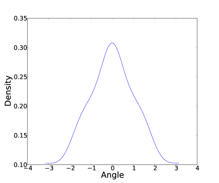
B)

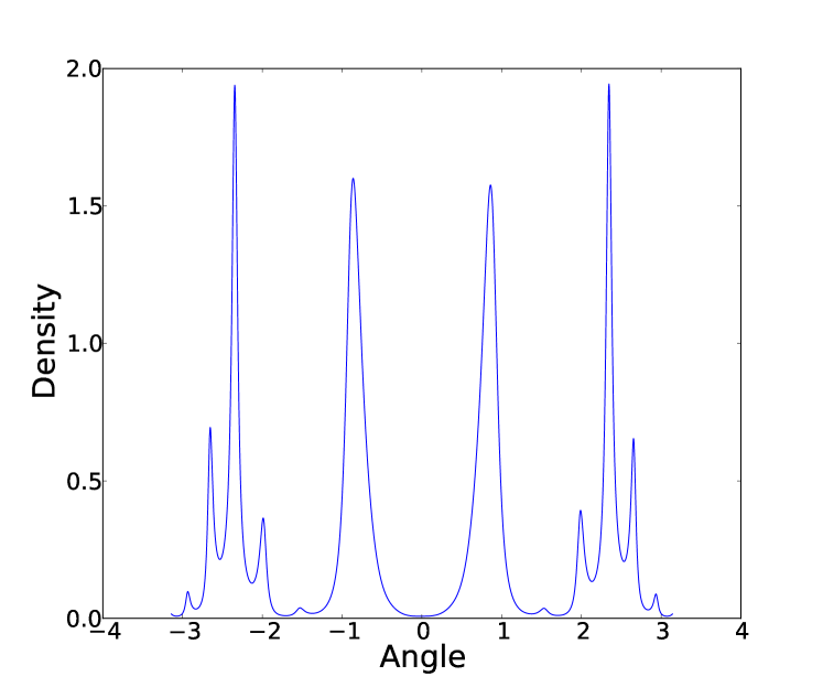
C)

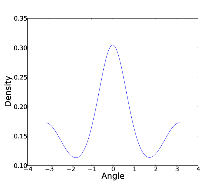
D)

Figure 1: The plots here show the equilibrium distributions calculated using the method in section B for the four systems. A) $\mathcal{B}_{1}$ and $\kappa_{1}$, B) $\mathcal{B}_{1}$ and $\kappa_{2}$, C) $\mathcal{B}_{2}$ and $\kappa_{1}$, and D) $\mathcal{B}_{2}$ and $\kappa_{2}$.

The first calculations run were to estimate the equilibrium distribution using the method in section B. The method was iterated until the $\|\cdot\|_{1}$ difference between successive iterations was less than double precision. The equilibrium distribution appeared to have a qualitatively stronger dependence on $\kappa$ than on $\mathcal{B}$ as can be seen in Figure 1.

A)

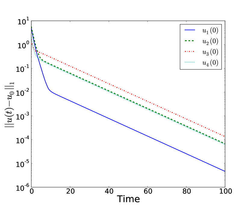
B)

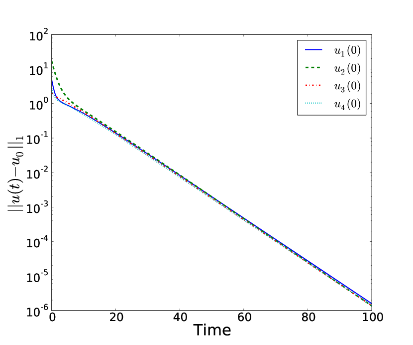
C)

D)

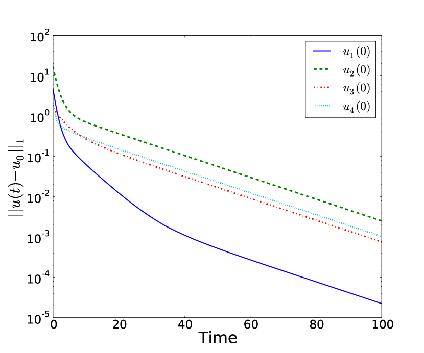
Figure 2: The observed $\mathnormal{L}^{1}$ distances from equilibrium as a function of time are plotted here on a log scale. The four lines on each plot each correspond to the solution starting with a different initial condition. A) $\mathcal{B}_{1}$ and $\kappa_{1}$. B) $\mathcal{B}_{1}$ and $\kappa_{2}$. C) $\mathcal{B}_{2}$ and $\kappa_{1}$. D) $\mathcal{B}_{2}$ and $\kappa_{2}$.

All of the simulations run converged (asymptotically) exponentially to the equilibrium. The equilibrium was calculated by iterating $\mathrm{A}^{\prime}$ as outlined in the following section. Figure 2 shows the $\mathnormal{L}^{1}$ distance between the simulation result and the calculated equilibrium on a log scale. The log scale was used to make the graphs legible and to show the exponential convergence. Moreover, all of the initial conditions appear to asymptotically converge at the same rate. That gives evidence that solutions are globally exponentially stable. The simulations provide evidence for exponential stability with some constant determined solely by $\mathcal{B}$ and $\kappa$.

4.2 Perturbation Expansion

The last approximate technique we will use is to study the perturbation expanion of the zeroth-order branching equation. For this section, we will again consider functions $u\in\mathnormal{L}^{1}$. However, we will again appeal to Hilbert space techniques when necessary.

Assume that the capping function can be written out as:

$$\kappa(\theta)=c+\varepsilon\phi(\theta)$$ (49)

where $\phi$ is smooth, has integral zero, and reasonably small so that $\varepsilon\phi$ is close to zero. The equation of motion is thus:

$$\dot{u}(\theta,t)=\frac{\Big{(}\mathcal{B}\star u\Big{)}(\theta,t)}{\int u(\omega,t)\,\mathrm{d}\omega}-(c+\varepsilon\phi(\theta))u(\omega,t)$$ (50)

For the Cauchy problem with $u(\theta,0)=u^{\star}(\theta)$, we will look for solutions of the form:

$$u(\theta,t)=\sum_{j=0}^{\infty}\varepsilon^{j}u_{j}(\theta,t)$$ (51)

with the initial conditions $u_{0}(\theta,0)=u^{\star}$ and $u_{j}(\theta,0)=0$ for all $j\geq 1$. Showing that both $u_{0}$ and $u_{1}$ converge to the equilibribium defined in equation (35) provides some evidence for the stability of the full equation.

First, we will calculate the first couple of terms of the equilibrium using equation (35):

$$\frac{\Big{(}\mathcal{B}\star w\Big{)}(\theta)}{1+\varepsilon\phi(\theta)}=\mu w(\theta)$$ (52)

where we have the two expansions:

$$w(\theta)=\sum_{j=0}^{\infty}\varepsilon^{j}w_{j}(\theta)\qquad\mu=\sum_{j=0}^{\infty}\varepsilon^{j}\mu_{j}$$ (53)

Expanding out the terms in (52) gives:

$$\left(\sum_{j=0}^{\infty}\frac{(-\varepsilon\phi)^{j}}{c^{j+1}}\right)\left(\sum_{j=0}^{\infty}\varepsilon^{j}\mathcal{B}\star w_{j}\right) =\left(\sum_{j=0}^{\infty}\varepsilon^{j}\mu_{j}\right)\left(\sum_{j=0}^{\infty}\varepsilon^{j}w_{j}\right)$$

$$\sum_{j=0}^{\infty}\varepsilon^{j}\sum_{k=0}^{j}\frac{(-\phi)^{k}}{c^{k+1}}\mathcal{B}\star w_{j-k} =\sum_{j=0}^{\infty}\varepsilon^{j}\sum_{k=0}^{j}\mu_{j}w_{j-k}$$ (54)

The first term ($\varepsilon^{0}$) is simply the eigenproblem for the unperturbed problem:

$$\mathcal{B}\star w_{0}=c\mu_{0}w_{0}$$ (55)

The only positive solution of the above is $\mu_{0}=\frac{1}{c}$ and $w_{0}$ constant. Since we know the equilibrium has the same integral as the eigenvalue, we know that $w_{0}=\frac{1}{c2\pi}$. The $\varepsilon^{1}$ term gives:

$$\frac{\mathcal{B}\star w_{1}}{c}-\frac{\phi\mathcal{B}\star w_{0}}{c^{2}}=\mu_{0}w_{1}+\mu_{1}w_{0}$$ (56)

Filling in the known quantities and rearranging gives:

$$\mathcal{B}\star w_{1}-w_{1}=\frac{\phi}{c}+\frac{\mu_{1}}{2\pi}$$ (57)

The left hand side is a self-adjoint Fredholm operator with nullspace spanned by the constant function, $w_{0}$. By the Fredholm alternative, we know that (57) is solvable if and only if the right hand side is orthogonal to $w_{0}$, i.e. $\phi(\theta)+\frac{\mu_{1}}{2\pi}$ has integral zero. To have integral zero, we know that $\mu_{1}=-\frac{2\pi}{c}\int\phi(\omega)\,\mathrm{d}\omega=0$.

We can write out $w_{1}$ in terms of the Neumann series. By hypothesis, $\phi$ is bounded, and therefore $\phi\in\mathnormal{L}^{2}$. We know that $\mathcal{B}\star$ has operator norm strictly less than one on the space of functions orthogonal to $w_{0}$: $\{w_{0}\}^{\perp}\subsetneq\mathnormal{L}^{2}$, which implies the Neumann series converges in $\mathnormal{L}^{2}$ norm:

$$w_{1}=\sum_{j=0}^{\infty}\mathrm{B}^{j}\phi$$ (58)

where $\mathrm{B}u=\mathcal{B}\star u$ and $\mathrm{B}^{j+1}u=\mathcal{B}\star\mathrm{B}^{j}u$. The above expansion implies that $\int w_{1}=0$. We know that $\int\mathrm{B}u=\int u$ which gives:

$$\int\sum_{j=0}^{n}\Big{(}\mathrm{B}^{j}\phi\Big{)}(\theta)\,\mathrm{d}\theta=0$$ (59)

Since norm convergence implies weak convergence, we can finish the proof by observing:

$$\lim_{n\to\infty}\int w_{1}-\int\sum_{j=0}^{n}\mathrm{B}^{j}\phi=\lim_{n\to\infty}\left\langle w_{1}(\theta)-\sum_{j=0}^{n}\mathrm{B}^{j}\phi,1\right\rangle=0$$ (60)

We can now consider the dynamics. We can write out (50) in terms of our power series:

$$\sum_{j=0}^{\infty}\varepsilon^{j}\dot{u}_{j}(\theta,t)=\frac{1}{\sum_{j=0}^{\infty}\varepsilon^{j}\int u_{j}(\omega,t)\,\mathrm{d}\omega}\sum_{j=0}^{\infty}\varepsilon^{j}\Big{(}\mathcal{B}\star u_{j}\Big{)}(\theta,t)\\ -(c+\varepsilon\phi(\theta))\sum_{j=0}^{\infty}\varepsilon^{j}u(\theta,t)$$ (61)

A formal treatment of the integrand could be considered, but without confidence of convergence, that seems unnecessary. We are only calculating $u_{0}$ and $u_{1}$, so we will ignore terms of $o(\varepsilon^{2})$ or higher in the integrand:

$$\sum_{j=0}^{\infty}\varepsilon^{j}\dot{u}_{j}(\theta,t)=\left(\sum_{j=0}^{\infty}\frac{\left(-\varepsilon\int u_{1}(\omega,t)\,\mathrm{d}\omega\right)^{j}}{\left(\int u_{0}(\omega,t)\,\mathrm{d}\omega\right)^{j+1}}\right)\left(\sum_{j=0}^{\infty}\varepsilon^{j}\Big{(}\mathcal{B}\star u_{j}\Big{)}(\theta,t)\right)\\ -\Big{(}c+\varepsilon\phi(\theta)\Big{)}\sum_{j=0}^{\infty}\varepsilon^{j}u_{j}(\theta,t)$$ (62)

The above equation allows us to solve for the first two terms of the perturbation expansion.

The equation for the first term $u_{0}(\theta,t)$ from the $\varepsilon^{0}$ expansion is:

$$\dot{u}_{0}(\theta,t)=\frac{\Big{(}\mathcal{B}\star u_{0}\Big{)}(\theta,t)}{\int u_{0}(\omega,t)\,\mathrm{d}\omega}-u_{0}(\theta,t)$$ (63)

We can explicitly solve for the time-dependent total density by observing:

$$\frac{\partial}{\partial t}\int u(\omega,t)\,\mathrm{d}\omega=1-\int u(\omega,t)\,\mathrm{d}\omega$$ (64)

Solving the above gives:

$$\int u(\omega,t)\,\mathrm{d}\omega=1+A\exp[-t]$$ (65)

where $A=\int u^{\star}(\omega)\,\mathrm{d}\omega$. Substituting in to (63) gives:

$$\dot{u}_{0}(\theta,t)=\frac{\Big{(}\mathcal{B}\star u_{0}\Big{)}(\theta,t)}{1+A\exp[-t]}-u_{0}(\theta,t)$$ (66)

The right hand side of the above clearly depends upon the denominator $1+A\exp[-t]$ continuously in almost any operator topology. Since we are primarily concerned with the asymptotic dynamics, it is sufficient to show that the asymptotic equation converges:

$$\dot{u}_{0}=\mathcal{B}\star u_{0}-u_{0}$$ (67)

From the results in Theorem 2, we know that the above equation converges to a multiple of the principal eigenfunction $w_{0}$. Equation (65) implies that the total density is equal to $\frac{1}{c}$ and $u_{0}(\theta,t)\to w_{0}(\theta)$ in norm as was required.

The second term of the expansion $(\varepsilon^{1})$ is slightly more complicated:

$$\dot{u}_{1}(\theta,t)=\frac{\Big{(}\mathcal{B}\star u_{1}\Big{)}(\theta,t)}{\int u_{0}(\omega,t)\,\mathrm{d}\omega}-\frac{\int u_{1}(\omega,t)\,\mathrm{d}\omega}{\left(\int u_{0}(\omega,t)\,\mathrm{d}\omega\right)^{2}}\Big{(}\mathcal{B}\star u_{0}\Big{)}(\theta,t)-u_{1}(\theta,t)-\phi(\theta)u_{0}(\theta,t)$$ (68)

Substituting in known quantities gives:

$$\dot{u}_{1}=\frac{\mathcal{B}\star u_{1}}{1+A\exp[-t]}-\frac{\int u_{1}}{(1+A\exp[-t])^{2}}\mathcal{B}\star u_{0}-u_{1}-\phi u_{0}$$ (69)

We can now solve for the integral of $u_{1}$:

$$\frac{\partial}{\partial t}\int u_{1} =\frac{\int\mathcal{B}\star u_{1}}{1+A\exp[-t]}-\frac{\int u_{1}}{1+A\exp[-t]}-\int u_{1}-\int\phi u_{0}$$

$$=-\int u_{1}-\int\phi u_{0}$$ (70)

That gives the explicit solution:

$$\int u_{1}(\omega,t)\,\mathrm{d}\omega=-\exp[-t]\int\limits_{0}^{t}\exp[s]\int\phi(\omega)u_{0}(\omega,t)\,\mathrm{d}\omega\,\mathrm{d}s$$ (71)

Weak convergence of $u_{0}\to w_{0}$ is sufficient to show that $\int u_{1}\to-\int\phi$. Substituting the asymptotic forms into (68) similar to the first term gives:

$$\dot{u}_{1}=\mathcal{B}\star u_{1}-u_{1}+\int\phi-\frac{\phi}{2\pi}$$ (72)

asymptotically. Finally, to show convergence, we can write $u_{1}$ as:

$$u_{1}(\theta,t)=w_{1}(\theta)+\epsilon(\theta,t)$$ (73)

where $\epsilon(\theta,0)=-w_{1}(\theta)$. Putting that form into (72) gives:

$$\dot{\epsilon}=\mathcal{B}\star\epsilon-\epsilon$$ (74)

Inspection of (57) shows that $w_{1}(\theta)$ is bounded and is therefore in $\mathnormal{L}^{2}$. Since $\mathcal{B}\star u-u$ has the Fourier eigenpairs $\{(\gamma_{n},\frac{1}{\sqrt{2\pi}}\exp[-in\theta])\}_{n\in\mathbb{N}}$ as an orthonormal basis, we can write the $\mathnormal{L}^{2}$ norm of $\varepsilon$ as:

$$\|\epsilon(\theta,t)\|_{2}^{2}=\sum_{n\in\mathbb{N}}\exp[\gamma_{n}t]|\hat{w}_{1}(n)|^{2}$$ (75)

where $\hat{w}_{1}(n)$ is the $n$’th Fourier component of $w_{1}(\theta)$. We know that $\gamma_{n}<0$ for all $n>0$ and $\sup_{n\geq 1}\gamma_{n}<0$. Combining those facts with the fact that $\hat{w}_{1}(0)=0$ because $\int w_{1}=0$ gives:

$$\|\epsilon(\theta,t)\|_{2}^{2}=\sum_{n\geq 1}\exp[\gamma_{n}t]|\hat{w}_{1}(n)|^{2}\leq\exp\left[\left(\sup_{n\geq 1}\gamma_{n}\right)t\right]\sum_{n\geq 1}|\hat{w}_{1}(n)|^{2}$$ (76)

That implies that $u_{1}(\theta,t)\to w_{1}(\theta)$ asymptotically exponentially.

We have now shown that the first two components of the perturbation expansion of (50) converge to an equilibrium. Calculating further terms would not provide any additional insight as the estimate from equation (54) gives a worse estimate after the first order. Recall from the proof of Proposition 13 that the integral of the equilibrium $w$ has to be equal to the eigenvalue $\mu$. However, it is easy to observe that the argument showing that $\int w_{1}=$ holds for all $w_{j}$, which implies that $\int\sum_{j=0}^{k}\varepsilon^{j}w_{j}=\frac{1}{c}$ for all $k$. However, $\sum_{j=0}^{k}\varepsilon^{j}\mu_{j}\neq\mu_{0}=\frac{1}{c}$ for all $k\geq 2$. We can show that by caclulating the second term in the perturbation expansion.

Using equation (54), we can gather the $\varepsilon^{2}$ terms:

$$\frac{1}{c}\mathcal{B}\star w_{2}-\frac{\phi}{c^{2}}\mathcal{B}\star w_{1}+\frac{\phi^{2}}{c^{3}}\mathcal{B}\star w_{0}=\mu_{0}w_{2}+\mu_{1}w_{1}+\mu_{2}w_{0}$$ (77)

Observe that $\mathcal{B}\star w_{1}=w_{1}+\frac{\phi}{c}$, and filling in other known quantities gives the relation:

$$\frac{1}{c}\left(\mathcal{B}\star w_{2}-w_{2}\right) =\frac{\phi}{c^{2}}\mathcal{B}\star w_{1}-\frac{\phi^{2}}{c^{3}}+\mu_{2}w_{0}$$

$$\mathcal{B}\star w_{2}-w_{2} =\frac{\phi^{2}}{c^{2}}-\frac{\phi^{2}}{c^{2}}+\frac{\phi w_{1}}{c}+\frac{\mu_{2}}{2\pi}$$

$$\mathcal{B}\star w_{2}-w_{2} =\frac{\phi w_{1}}{c}+\frac{\mu_{2}}{2\pi}$$ (78)

It is obvious that $\mu_{2}=0\iff\int\phi w_{1}=0$. However, we can observe that:

$$\int\frac{\phi w_{1}}{c}=\int\phi\left(\mathrm{B}-\mathrm{I}\right)^{-1}\frac{\phi}{c} =\left\langle\phi,\left(\mathrm{B}-\mathrm{I}\right)^{-1}\frac{\phi}{c}\right\rangle$$

$$=\Big{\langle}(\mathrm{B}-\mathrm{I})w_{1},(\mathrm{B}-\mathrm{I})(\mathrm{B}-\mathrm{I})^{-1}w_{1}\Big{\rangle}$$

$$=\Big{\langle}(\mathrm{B}-\mathrm{I})w_{1},w_{1}\Big{\rangle}$$ (79)

by observing that $(\mathrm{B}-\mathrm{I})w_{1}=\frac{\phi}{c}$. We can use the Cauchy-Schwarz inequality to show:

$$\langle\mathrm{B}w_{1},w_{1}\rangle-\langle w_{1},w_{1}\rangle\leq\|\mathrm{B}w_{1}\|_{2}\|w_{1}\|_{2}-\|w_{1}\|_{2}^{2}<0$$ (80)

The last inequality comes from the fact that $\|\mathrm{B}f\|_{2}\leq\|\mathrm{B}\|\|f\|_{2}=\|f\|_{2}$ and that equality holds if and only if $f\equiv C$.

An explicit example can give insight into the non-convergence discussed in the previous paragraph. Assume $\mathcal{B}=\frac{1}{2\pi}$ and $\kappa=1+\varepsilon\phi$ where $|\varepsilon\phi|<1$. It is easy to see that the principal solution to (52) is $w=\frac{1}{1+\varepsilon\phi}$ and $\mu=\int\frac{1}{1+\varepsilon\phi}$. Moreover, we have the exact expansion in $\varepsilon$:

$$w=\sum_{j=0}^{\infty}\varepsilon^{j}w_{j}=\sum_{j=0}^{\infty}\varepsilon^{2}(-\phi)^{j}$$ (81)

By our hypothesis $|\varepsilon\phi|<1$, we know the above converges. It is easy to see that:

$$(\mathrm{B}-\mathrm{I})^{-1}\phi=-\sum_{j=0}^{\infty}\mathrm{B}^{j}\phi=-\phi$$ (82)

which is the exact solution for the first term of the asymptotic expansion. However, the second term gives an incorrect solution:

$$(\mathrm{B}-\mathrm{I})^{-1}\left(\phi^{2}-\int\phi^{2}\right) =\sum_{j=0}^{\infty}\mathrm{B}\left(\int\phi^{2}-\phi^{2}\right)$$

$$=\int\phi^{2}(\omega)\,\mathrm{d}\omega-\phi^{2}(\theta)\neq\phi^{2}(\theta)$$ (83)

Further terms would show the same difficulty.

5 Conclusions

The results presented here provide a reference point for future work on the orientation patterns of branching actin networks. Given the current models, it would seem that factors external to the actin network determine the distinct orientation patterns observed in experiment. In experiments where the cell goes through protrusion/retraction cycles, different orientation patterns are observed at different points in the cycle [13]. One possible factor leading to the varying patterns may be how the network deals with the load from the cell membrane [29].

In the numerical results, only $\mathcal{B}_{1}$ and $\kappa_{1}$ were physically based, but Figure 1 show that there is a complex interplay between the capping and branching functions to result in the equilibrium distribution. The stability seen in Figure 2 may indicate why the orientation patterns seen in experiment have been so stable. The numerical results also reinfoce the analytical result that there is only one stable orientation pattern, in contrast with the multiple equilibria hypothesis in Weichsel and Schwarz [31].

Appendix A Methods

All simulations were run using the Numpy [2, 20, 21, 14] extension to Python. The equations of motion were integrated using a simple Euler method. The simulations were run for 100 time units with a time step of 0.01 time units. The circle was discretized using $2^{11}$ equally spaced points from $-\pi$ to $\pi$ (the power of 2 was used to speed up the fast Fourier transform). All integrals were taken using the trapezoidal method included in Numpy. The convolution was performed by taking the real fast Fourier transform of the branching kernel $\mathcal{B}$ and the density $u(\theta,t)$, multiplying, and taking the inverse real fast Fourier transform. The built-in Numpy fast convolution method was not used because that method pads the two convolved functions with extra zeros to prevent circular convolution, but the equations used here explicitly call for the circular convolution. The convolution was normalized by dividing $\mathcal{B}$ by the integral of the convolution of $\mathcal{B}$ with the constant function $\mathcal{B}\star\frac{1}{2\pi}$. Finally, the total branching rate was normalized by integrating the density at the previous time step, i.e.:

$$u(\theta,t+\,\mathrm{d}t)=\,\mathrm{d}t\left(\frac{\Big{(}\mathcal{B}\star u\Big{)}(\theta,t)}{\int u(\theta,t)\,\mathrm{d}\theta}-\kappa(\theta)u(\theta,t)\right)$$ (84)

Using the integral from the previous time step and not a more sophisticated prediction-correction methods is justified by the following inequality:

$$|u(\theta,t+\,\mathrm{d}t)-u(\theta,t)| \leq\,\mathrm{d}t\left(\int\Big{(}\mathcal{B}\star u\Big{)}(\theta,t)\,\mathrm{d}\theta+\int\kappa(\theta)u(\theta,t)\,\mathrm{d}\theta\right)$$

$$\leq\Big{(}1+\sup_{\theta\in S^{1}}\kappa(\theta)\Big{)}\,\mathrm{d}t\|u(\theta,t)\|_{1}\leq 3\,\mathrm{d}t\|u(\theta,t)\|_{1}$$ (85)

Since simulations remain bounded, the bound above can be made uniform.

The equilibrium was calculated a priori by iterating the equilibrium operator $\mathrm{A}^{\prime}$. Explicitly, a sequence of functions was generated by:

$$v_{n+1}(\theta)=\frac{1}{\int v_{n}(\theta)\,\mathrm{d}\theta}\mathrm{A}^{\prime}v_{n}(\theta)$$ (86)

where the discretization and convolution were performed exactly as above and $v_{0}=\frac{1}{2\pi}$. The theoretical justification for using this method is outlined in Section B. For three combinations of $\mathcal{B}$ and $\kappa$, $\|v_{10^{4}}-v_{2\times 10^{4}}\|_{1}$ was less than numerical precision. For the combination of $\mathcal{B}_{1}$ and $\kappa_{2}$, $v_{10^{4}}$ was not sufficiently converged, so $v_{10^{6}}$ was used. That decision was based on the condition that $\|v_{10^{6}}-v_{2\times 10^{6}}\|_{1}$ was less than numerical precision. That level of precision was used to ensure that the convergence could be seen even when $\|u(\theta,t)-v_{n}\|_{1}\leq 10^{-6}-10^{-10}$. Even $10^{6}$ iterations of $\mathrm{A}^{\prime}$ only took several minutes on a standard Linux desktop system concurrently running other programs, a number that could be reduced with further optimization.

At each time-step, the $\mathnormal{L}^{1}$ distance between the state of the system $u(\theta,t)$ and the equilibrium was calculated. That quantity is plotted as a function of time in Figure 2.

Appendix B Calculating Equilibrium Distributions

The results in this article justify the use of a naive eigenvalue calculation algorithm. Calculating eigenvalues of integral equations is a non-trivial problem. Investigation into open questions regarding the generality of orientation patterns across branching and capping patterns, such as in [24], may require calculating the equilibrium solution to equations like the ones analyzed here. Moreover, in the previous section, equilibrium distributions were calculated a priori to show that simulations converged. The method below has proven to be very efficient for the work in this article.

We will consider calculating the leading eigenvalue of the equilibrium operator for zeroth-order branching, $\mathrm{A}^{\prime}$. As $\mathrm{A}^{\prime}$ is self-adjoint and compact, we can represent its range as the sum of eigenfunctions. We can explicitly calculate the $n$-th iterate of $\mathrm{A}^{\prime}$ in terms of its (orthonormal) eigenfunctions:

$$\Big{(}\mathrm{A}^{\prime}\Big{)}^{n}v=\Big{(}\mathrm{A}^{\prime}\Big{)}^{n}\Big{(}\sum_{j}c_{j}u_{j}\Big{)}=\sum_{j}\mu_{j}^{n}c_{j}u_{j}$$ (87)

where $c_{j}=\langle v,u_{j}\rangle_{\kappa}$. We know that $\mu_{0}$ is equal to the spectral radius from the Krein-Rutman theorem as in the proof of Theorem 2. The proof also implies the eigenvalue is simple. Finally, since $\mathrm{A}^{\prime}$ is a compact operator, we know that there must be a spectral gap, i.e. $\mu_{0}-|\mu_{j}|>c>0$ for some $c$ and all $j\neq 0$.

All that remains necessary to show that the above iteration converges to the positive equilibrium is to show that $c_{j}=\langle v,u_{0}\rangle_{\kappa}\neq 0$. If $v$ equals the constant function, that condition is fulfilled. However, a stronger result is possible. By a result in [8], we know that $u_{0}(\theta)>0$. The continuity of $u_{0}$ gives that $\inf u_{0}>0$. Thus, we have the inequality:

$$\langle v,u_{0}\rangle_{\kappa}\geq\inf_{\theta\in S^{1}}(u_{0}(\theta)\kappa(\theta))\int\limits_{S^{1}}v(\theta)\,\mathrm{d}\theta>0$$ (88)

which implies that the iterative procedure will converge.

References

- [1] Wolfgang Arendt. Resolvent positive operators. Proceedings of the London Mathematical Society, s3-54(2):321–349, 1987.
- [2] David Ascher, Paul F. Dubois, Konrad Hinsen, James Hugunin, and Travis Oliphant. Numerical Python. Lawrence Livermore National Laboratory, Livermore, CA, ucrl-ma-128569 edition, 1999.
- [3] C. T. H. Baker. The Numerical Treatment of Integral Equations. Clarendon Press, Oxford, 1977.
- [4] R. Ben-Yishai, R. L. Bar-Or, and H. Sompolinsky. Theory of orientation tuning in visual cortex. Proc Natl Acad Sci U S A, 92(9):3844–3848, 1995.
- [5] P. Bressloff. Euclidean shift-twist symmetry in population models of self-aligning objects. SIAM Journal on Applied Mathematics, 64(5):1668–1690, 2004.
- [6] Yves Capdeboscq. Homogenization of a neutronic critical diffusion problem with drift. Proceedings of the Royal Society of Edinburgh, Section: A Mathematics, 132:567–594, 6 2002.
- [7] Anders E. Carlsson. Actin dynamics: From nanoscale to microscale. Annual Review of Biophysics, 39(1):91–110, 2010.
- [8] A. De Masi, E. Olivieri, and E. Presutti. Spectral properties of integral operators in problems of interface dynamics and metastability. Markov Processes and Related Fields, 4(1):27–112, 1998.
- [9] Roberto Dominguez and Kenneth C. Holmes. Actin structure and function. Annual Review of Biophysics, 40(1):169–186, 2011.
- [10] Z. Drmac. Applied Mathematics and Scientific Computing. Springer, 2003.
- [11] L. Edelstein-Keshet and B. Ermentrout. Models for branching networks in two dimensions. SIAM Journal on Applied Mathematics, 49(4):1136–1157, 1989.
- [12] Edith Geigant, Karina Ladizhansky, and Alexander Mogilner. An integrodifferential model for orientational distributions of f-actin in cells. SIAM Journal on Applied Mathematics, 59(3):pp. 787–809, 1998.
- [13] Grégory Giannone, Benjamin J Dubin-Thaler, Hans-Günther Döbereiner, Nelly Kieffer, Anne R Bresnick, and Michael P Sheetz. Periodic lamellipodial contractions correlate with rearward actin waves. Cell, 116(3):431–443, 2004.
- [14] Eric Jones, Travis Oliphant, Pearu Peterson, et al. SciPy: Open source scientific tools for Python, 2001–.
- [15] I. V. Maly and G. G. Borisy. Self-organization of a propulsive actin network as an evolutionary process. Proc Natl Acad Sci U S A, 98(20):11324–11329, Sep 2001.
- [16] A. Mogilner, L. Edelstein-Keshet, and G. B. Ermentrout. Selecting a common direction. ii. peak-like solutions representing total alignment of cell clusters. J Math Biol, 34(8):811–842, 1996.
- [17] Alex Mogilner and Leah Edelstein-Keshet. Selecting a common direction. Journal of Mathematical Biology, 33:619–660, 1995.
- [18] Alex Mogilner and George Oster. Force generation by actin polymerization ii: the elastic ratchet and tethered filaments. Biophys J, 84(3):1591–1605, 2003.
- [19] R. D. Mullins, J. A. Heuser, and T. D. Pollard. The interaction of arp2/3 complex with actin: nucleation, high affinity pointed end capping, and formation of branching networks of filaments. Proc Natl Acad Sci U S A, 95(11):6181–6186, 1998.
- [20] Travis E. Oliphant. Guide to NumPy. Provo, UT, 2006.
- [21] Travis E. Oliphant. Python for scientific computing. Computing in Science & Engineering, 9(3):10–20, 2007.
- [22] Benoît Perthame. Transport Equations in Biology (Frontiers in Mathematics). Birkhäuser Basel, 1 edition, November 2006.
- [23] T. D. Pollard, L. Blanchoin, and R. D. Mullins. Molecular mechanisms controlling actin filament dynamics in nonmuscle cells. Annu Rev Biophys Biomol Struct, 29:545–576, 2000.
- [24] D. Quint and J. Schwarz. Optimal orientation in branched cytoskeletal networks. Journal of Mathematical Biology, 63:735–755, 2011.
- [25] Susanne M Rafelski and Julie A Theriot. Crawling toward a unified model of cell mobility: spatial and temporal regulation of actin dynamics. Annu Rev Biochem, 73:209–239, 2004.
- [26] Sébastien Schaub, Jean-Jacques Meister, and Alexander B Verkhovsky. Analysis of actin filament network organization in lamellipodia by comparing experimental and simulated images. J Cell Sci, 120(Pt 8):1491–1500, 2007.
- [27] Thomas E Schaus and Gary G Borisy. Performance of a population of independent filaments in lamellipodial protrusion. Biophys J, 95(3):1393–1411, 2008.
- [28] Thomas E Schaus, Edwin W Taylor, and Gary G Borisy. Self-organization of actin filament orientation in the dendritic-nucleation/array-treadmilling model. Proc Natl Acad Sci U S A, 104(17):7086–7091, 2007.
- [29] Daniel B Smith and Jian Liu. Branching and capping determine the force-velocity relationships of branching actin networks. Physical Biology, 10(1):016004, 2013.
- [30] Alexander B. Verkhovsky, Oleg Y. Chaga, Sébastien Schaub, Tatyana M. Svitkina, Jean-Jacques Meister, and Gary G. Borisy. Orientational order of the lamellipodial actin network as demonstrated in living motile cells. Molecular Biology of the Cell, 14(11):4667–4675, 2003.
- [31] Julian Weichsel and Ulrich S. Schwarz. Two competing orientation patterns explain experimentally observed anomalies in growing actin networks. Proceedings of the National Academy of Sciences, 107(14):6304–6309, 2010.
- [32] Julian Weichsel, Edit Urban, J. Victor Small, and Ulrich S Schwarz. Reconstructing the orientation distribution of actin filaments in the lamellipodium of migrating keratocytes from electron microscopy tomography data. Cytometry A, 81(6):496–507, 2012.
- [33] K. Zhang. Representation of spatial orientation by the intrinsic dynamics of the head-direction cell ensemble: a theory. J Neurosci, 16(6):2112–2126, 1996.