Dynamics of a superconducting qubit coupled to the quantized cavity field: a unitary transformation approach

Abstract

We present a novel approach for studying the dynamics of a superconducting qubit in a cavity. We succeed in linearizing the Hamiltonian through the application of an appropriate unitary transformation followed by a rotating wave approximation (RWA). For certain values of the parameters involved, we show that it is possible to obtain a a Jaynes-Cummings type Hamiltonian. As an example, we show the existence of super-revivals for the qubit inversion.

1 Introduction

Superconducting qubits, which consist of a small superconducting electrode connected to a reservoir via a Josephson junction yu01 , are considered to be promising qubits for quantum information processing. Because of the charging effect in the small electrode, the two charge-number states, in which the number of Cooper pairs in the“box” electrode differs by one, constitute an effective two-level system. These “artificial atoms,” with well-defined discrete energy levels, provide a platform to test fundamental quantum effects, e.g., related to cavity quantum electrodynamics (cavity QED) as well as for quantum information schemes. A particularly interesting proposal is a viable architecture for quantum computation based on circuit cavity QED, as presented in blais04 . A few quantum features of that system have been already experimentally demonstrated some years ago; for instance, the generation of superposition of the two charge states bouchiat98 ; nakamura97 , and coherent oscillations between two degenerate states nakamura99 . More recently, an important step for reaching the quantum regime in such systems has been achieved: the strong coupling of the quantized radiation field to a superconducting qubit, as experimentally demonstrated by A. Wallraff et al. wallraff04 . Accordingly, a superconducting qubit coupled to the quantized field may be used to engineer quantum states; for instance, as a deterministic single-photon source as well as to generate arbitrary superpositions of Fock states of the cavity field, as proposed in yu04 . As a matter of fact, the generation of Fock (and coherent) states has been already performed in such systems houck07 ; hofheinz08 . We may also cite as important developments involving superconducting systems appplied to quantum information schemes, the demonstrations of quantum buses using superconducting qubits and photons sillanpaa07 ; majer07 , the implementation of two-qubit algorithms dicarlo09 , the encoding of quantum information in Schrödinger type cat states vlastakis13 , as well as the deterministic entanglement of superconducting qubits riste13 . Moreover, it has also become possible to engineer an artificial nonlinear Kerr-type medium, allowing the observation of quantum state collapses and revivals kirchmair13 .

In this paper we investigate a model of circuit QED following reference yu04 : a single mode cavity field in the microwave regime, with photon transitions between the ground and first excited states of a two-level system formed by a superconducting quantum interference device (SQUID). This artificial two-level“atom” can be easily controlled by an applied gate voltage $V_{g}$ and the flux $\Phi_{c}$ generated by the classical magnetic field through the SQUID. Here we adopt a new approach to this problem: we depart from the full radiation field and supercondutor interaction Hamiltonian, and apply a unitary transformation similar to the one introduced in moya . After transforming the original Hamiltonian, we show that it is possible to obtain a simpler Hamiltonian by performing a rotating wave approximation (RWA); we are able to obtain a Jaynes-Cummings like Hamiltonian which makes possible to solve the problem analytically without making any further approximations. In other words, we were able to linearize the superconductor/quantized field Hamiltonian without doing the usual power series expansions of the Hamiltonian itself, as usually found in the literature yu04 .

2 The model

We consider a system constituted by a SQUID type superconducting box with $n_{c}$ excess Cooper-pair charges connected to a superconducting loop via two identical Josephson junctions having capacitors $C_{J}$ and coupling energies $E_{J}$. An external control voltage $V_{g}$ couples to the box via a capacitor $C_{g}$. We also assume that the system operates in a regime, consistent with most experiments involving charge qubits, in which only Cooper pairs coherently tunnel in the junctions. Therefore the system Hamiltonian may be written as yu01

$$H_{qb}=4E_{ch}(n_{c}-n_{g})^{2}-2E_{j}\cos(\frac{\pi\Phi_{X}}{\Phi_{0}})\cos(\Theta),$$ (1)

where $E_{ch}=e^{2}/2(C_{g}+2C_{J})$ is the single-electron charging energy, $n_{g}=C_{g}V_{g}/2e$ is the dimensionless gate charge (controlled by $V_{g}$), $\Phi_{X}$ is the total flux through the SQUID loop and $\Phi_{0}$ the flux quantum. By adjusting the flux through the superconducting loop, one may control the Josephson coupling energy as well as switch on and off the qubit-field interaction. The phase $\Theta=(\phi_{1}+\phi_{2})/2$ is the quantum-mechanical conjugate of the number operator $n_{c}$ of the Cooper pairs in the box, where $\phi_{i}$ (i = 1, 2) is the phase difference for each junction. The superconducting box is assumed to be working in the charging regime and the superconducting energy gap $\Delta$ is considered to be the largest energy involved. Moreover, the temperature $T$ is low enough so that the condition $\Delta\gg k_{B}T$ holds. The superconducting box then becomes an effective two-level system with states $|g\rangle$ (for $n_{c}=0$) and $|e\rangle$ (for $n_{c}=1$) given that the gate voltage is near a degeneracy point ($n_{g}=1/2$) yu01 and the quasi-particle excitation is completely suppressed averin .

If that circuit is placed within a single-mode microwave superconducting cavity, the qubit can be coupled to both a classical magnetic field (generates a flux $\Phi_{c}$) and the quantized cavity field (generates a flux $\Phi_{q}=\eta a+\eta^{*}a^{{\dagger}}$, with $a$ and $a^{{\dagger}}$ the annihilation and creation operators), being the total flux through the SQUID $\Phi_{X}=\Phi_{c}+\Phi_{q}$ you03 . The parameter $\eta$ is related to the mode function of the cavity field. The system Hamiltonian will then read

$$H=\hbar\omega a^{{\dagger}}a+E_{z}\sigma_{z}-E_{J}(\sigma_{+}+\sigma_{-})\cos\big{(}\gamma I+\beta a+\beta^{*}a^{{\dagger}}\big{)},$$ (2)

where we have defined the parameters $\gamma=\pi\Phi_{c}/\Phi_{0}$ and $\beta=\pi\eta/\Phi_{0}$. The first term corresponds to the free cavity field with frequency $\omega=4E_{ch}/\hbar$ and the second one to the qubit having energy $E_{z}=-2E_{ch}(1-2n_{g})$ with $\sigma_{z}=|e\rangle\langle e|-|g\rangle\langle g|$. The third term is the (nonlinear) photon-qubit interaction term which may be controlled by the classical flux $\Phi_{c}$. In general the Hamiltonian in equation (2) is linearized under some kind of assumption. In yu04 , for instance, the authors decomposed the cosine in Eq.(2) and expanded the terms $\sin[\pi(\eta\,a+H.c.)/\Phi_{0}]$ and $\cos[\pi(\eta\,a+H.c.)/\Phi_{0}]$ as power series in $a\,(a^{\dagger})$. In this way, if the limit $|\beta|\ll 1$ is taken, only single-photon transition terms in the expansion are kept, and a Jaynes-Cummings type Hamiltonian (JCM) is then obtained. Here, in contrast to that, we adopt a similar technique to the one presented in reference moya ; we obtain a linear, JCM-type Hamiltonian by first applying a transformation to the full Hamiltonian in equation (2) and making approximations afterwards. The suitable unitary transformation is given by

$$T = \frac{1}{\sqrt{2}}\Big{\{}-\frac{1}{2}\Big{[}D^{{\dagger}}\Big{(}\alpha,\gamma\Big{)}-D\Big{(}\alpha,\gamma\Big{)}\Big{]}I$$ (3)

$$- \frac{1}{2}\Big{[}D^{{\dagger}}\Big{(}\alpha,\gamma\Big{)}+D\Big{(}\alpha,\gamma\Big{)}\Big{]}\sigma_{z}$$

$$+ D\Big{(}\alpha,\gamma\Big{)}\sigma_{+}+D^{{\dagger}}\Big{(}\alpha,\gamma\Big{)}\sigma_{-}\Big{\}},$$

with $D(\alpha,\gamma)=D(\alpha)e^{i\frac{\gamma}{2}}$, where $D(\alpha)=\exp[(\alpha a^{{\dagger}}-\alpha^{*}a)]$ is Glauber’s displacement operator, with $\alpha=i\beta^{*}/2$. We obtain the following transformed Hamiltonian

$$H_{T} \equiv THT^{\dagger}$$ (4)

$$= \hbar\omega a^{{\dagger}}a+\frac{E_{J}}{2}\sigma_{z}+i\frac{\hbar}{2}\big{[}\omega\big{(}\beta a-\beta^{*}a^{{\dagger}}\big{)}+2i\frac{E_{z}}{\hbar}\big{]}\big{(}\sigma_{+}+\sigma_{-}\big{)}$$

$$+ \frac{E_{J}}{2}\cos\big{[}2\big{(}\beta a+\beta^{*}a^{{\dagger}}\big{)}+2\gamma\big{]}\sigma_{z}$$

$$- i\frac{E_{J}}{2}\sin\big{[}2\big{(}\beta a+\beta^{*}a^{{\dagger}}\big{)}+2\gamma\big{]}\big{(}\sigma_{+}-\sigma_{-}\big{)}.$$

It is worth mentioning that the same setup and transformation given by (3) may also be employed (see reference dago12 ) in a scheme for preparation of superpositions of coherent states of a single-mode cavity field (Schrödinger cats), extending the approach of Ref.yupra05 .

Now we rewrite $H_{T}$ in an interaction representation in the transformed space, or $H_{TI}=U_{0T}^{\dagger}V_{T}U_{0T}$, where

$$V_{T} = i\frac{\hbar}{2}\big{[}\omega\big{(}\beta a-\beta^{*}a^{{\dagger}}\big{)}+2i\frac{E_{z}}{\hbar}\big{]}\big{(}\sigma_{+}+\sigma_{-}\big{)}$$

$$+ \frac{E_{J}}{2}\cos\big{[}2\big{(}\beta a+\beta^{*}a^{{\dagger}}\big{)}+2\gamma\big{]}\sigma_{z}$$

$$- i\frac{E_{J}}{2}\sin\big{[}2\big{(}\beta a+\beta^{*}a^{{\dagger}}\big{)}+2\gamma\big{]}\big{(}\sigma_{+}-\sigma_{-}\big{)}$$

and $U_{0T}=e^{-i(\omega a^{{\dagger}}a+\frac{E_{J}}{2\hbar}\sigma_{z})t}$. We then obtain the transformed Hamiltonian in the interaction representation

$$H_{TI} = \frac{i\hbar\omega}{2}\Big{[}\Big{(}\beta a\sigma_{+}e^{-i(\omega-E_{J}/\hbar)t}-\beta^{*}a^{\dagger}\sigma_{-}e^{i(\omega-E_{J}/\hbar)t}\Big{)}$$ (6)

$$- \Big{(}\beta^{*}a^{\dagger}\sigma_{+}e^{i(\omega+E_{J}/\hbar)t}-\beta a\sigma_{-}e^{-i(\omega+E_{J}/\hbar)t}\Big{)}\Big{]}$$

$$- E_{z}\Big{(}\sigma_{+}e^{E_{J}/\hbar t}+\sigma_{-}e^{-E_{J}/\hbar t}\Big{)}$$

$$+ \frac{E_{J}}{2}\cos\Big{[}2\Big{(}\beta^{*}a^{\dagger}e^{i\omega t}+\beta ae^{-i\omega t}\Big{)}+2\gamma\Big{]}\sigma_{z}$$

$$- i\frac{E_{J}}{2}\sum_{n=0}^{\infty}\frac{{(2i)}^{2n}}{(2n)!}\Big{\{}\Big{\{}\sin(2\gamma)e^{i\frac{E_{J}}{\hbar}t}+\frac{2\cos(2\gamma)}{(2n+1)}$$

$$\times \Big{[}\beta^{*}a^{\dagger}e^{i(\omega+E_{J}/\hbar)t}+\beta ae^{-i(\omega+E_{J}/\hbar)t}\Big{]}\Big{\}}$$

$$\times \Big{[}\beta^{*2}a^{\dagger 2}e^{2i\omega t}+\beta^{2}a^{2}e^{-2i\omega t}$$

$$+ |\beta|^{2}(aa^{\dagger}+a^{\dagger}a)\Big{]}^{n}\sigma_{+}-h.c\Big{\}}.$$

3 Resonance condition: Jaynes-Cummings type Hamiltonian

At this stage we have in hands a transformed Hamiltonian equation (6) with a more complicated structure than the original one, in equation (2). Nevertheless, our new Hamiltonian may be considerably simplified by choosing an appropriate resonance condition and then applying the RWA. In fact, it is possible to obtain a well known Hamiltonian of quantum optical resonance: the Jaynes-Cummings Hamiltonian in the transformed frame. If the cavity frequency is such that $\hbar\omega=E_{J}$ and the parameter $\gamma$ (which may be controlled by the classical flux) equals $\gamma=\pi/4$ rad, the rapidly oscillating terms in the right hand side of equation (6) may be neglected (RWA), and the transformed Hamiltonian above reduces to

$$H_{TI,1}\approx-i\hbar(g^{*}a^{{\dagger}}\sigma_{-}-ga\sigma_{+}),$$ (7)

which coincides with the Jaynes-Cummings Hamiltonian with effective coupling constant $|g|=|\beta|\omega/2$. Now, in order to allow the RWA, the parameter $\beta$ cannot be arbitrarily large. In fact, an analogue of the strong coupling regime requires that $|g|\ll\omega$, or $|\beta|\ll 1$. Note that in the approach of reference yu04 , the condition $|\beta|\ll 1$ is also necessary, but for a different reason, i.e., to truncate the co-sine (sine) series; see, for instance, the discussion after equation (2). We should remark that in our scheme the Jaynes-Cummings evolution takes place in the transformed frame, differently from the model developed in yu04 .

Now we would like to discuss some aspects of the dynamics of the system. Despite of the fact that we have obtained a Jaynes-Cummings type Hamiltonian in the transformed space, the system dynamics is closely related to the dynamics of the driven Jaynes-Cummings model (DJCM), instead. In this case, the time evolution of the state vector, for an initial state $|\psi(0)\rangle$ is

$$|\psi(t)\rangle=T^{\dagger}{U}_{0T}(t){U}_{I}(t)T|\psi(0)\rangle,$$ (8)

where ${U}_{I}(t)$ is the Jaynes-Cummings evolution operator sten73 in the interaction representation

$${U}_{I}(t) = \frac{1}{2}\left[{C}_{n+1}+{C}_{n}\right]I+\frac{1}{2}\left[{C}_{n+1}-{C}_{n}\right]\sigma_{z}$$ (9)

$$+ \frac{\beta}{|\beta|}S_{n+1}a\sigma_{+}-\frac{\beta^{*}}{|\beta|}a^{\dagger}S_{n+1}\sigma_{-},$$

with ${C}_{n+1}=\cos\left(|g|t\sqrt{aa^{\dagger}}\right)$ and $S_{n+1}=\sin\left(|g|t\sqrt{aa^{\dagger}}\right)/{\sqrt{aa^{\dagger}}}$.

Now we may calculate the qubit inversion $W(t)=\langle\sigma_{z}\rangle$, having an initial state $|\psi(0)\rangle=|e\rangle\otimes|\alpha_{0}\rangle$, i.e., the qubit in the excited state and the field in a coherent state hofheinz08 with amplitude $\alpha_{0}$. The qubit inversion reads

$$W(t) = \frac{1}{2}\exp(-|\alpha_{0}-\beta|^{2})\sum_{n=0}^{\infty}\frac{|\alpha_{0}-\beta|^{2n}}{n!}\Big{\{}$$ (10)

$$2\cos\Big{(}\frac{E_{J}}{\hbar}t\Big{)}c_{n+1}c_{n}+\frac{n!}{\sqrt{n!(n+1)!}}$$

$$\times \Big{[}(\alpha_{0}^{\star}-\beta^{\star})e^{i\frac{E_{J}}{\hbar}t}+(\alpha_{0}-\beta)e^{-i\frac{E_{J}}{\hbar}t}\Big{]}$$

$$\times (c_{n+2}-c_{n})s_{n+1}-\frac{n!}{\sqrt{n!(n+2)!}}\Big{[}$$

$$( \alpha_{0}^{\star}-\beta^{\star})^{2}e^{i\frac{E_{J}}{\hbar}t}+(\alpha_{0}-\beta)^{2}e^{-i\frac{E_{J}}{\hbar}t}\Big{]}$$

$$\times s_{n+2}s_{n+1}\Big{\}},$$

where $c_{n}=\cos(gt\sqrt{n})$ and $s_{n}=\sin(gt\sqrt{n})$. In equation (10) the parameter $\beta$ was considered real for simplicity.

The structure of the equation above is similar to the one obtained for $\langle\sigma_{z}\rangle$ in the DJCM hmcsmd94 . Therefore we expect the phenomenon of super-revivals to be present in the qubit-cavity system, analogously to the DJCM. Super-revivals are revivals ocurring at larger time-scales than that of ordinary JCM revivals, and which sometimes arise in the atom-field dynamics hmcsmd94 . This peculiar behavior is illustrated in figure (1) and figure (2). We note that the existence or not of super-revivals is narrowly connected to the preparation of the initial field state. For instance, if we have $\alpha_{0}=(5.0,0.5)$, the super-revivals do not occur [see Fig. (1)], and we have ordinary revivals only. However, for $\alpha_{0}=(0.5,5.0)$, super-revivals take place in that system, as seen in Fig. (2).

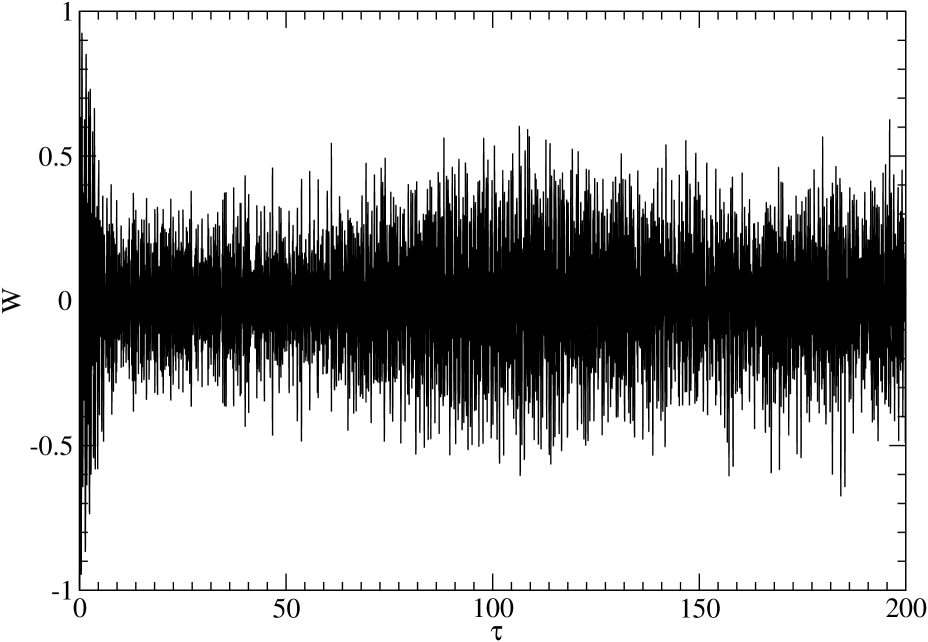
Figure 1: Plot of the qubit inversion as a function of the (dimensionless) scaled time $\tau=gt$. Ordinary revivals occurring for $\alpha_{0}=(5.0,0.5)$ and $\beta=0.02$.

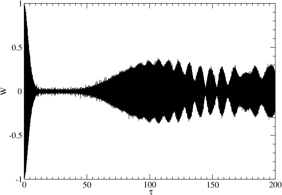
Figure 2: Plot of the qubit inversion as a function of the (dimensionless) scaled time $\tau=gt$. Super-revivals occurring for $\alpha_{0}=(0.5,5.0)$ and $\beta=0.02$.

Regarding the influence of an external environment, we know that in a non-ideal system, decoherence normally deteriorates quantum effects. In this paper, though, we have studied the ideal system (without an environment), in order to identify its main features. Nevertheless we would like to make a few comments about the non-ideal situation. Real cavities have losses, which are usually modelled by coupling the cavity field to an external thermal bath. A typical interaction term describing such a coupling may be written as (under the rotating wave approximation), $\sum_{i}\left(\lambda_{i}a^{\dagger}b_{i}+\lambda_{i}^{*}ab_{i}^{\dagger}\right)$, where the operators $b_{i},b_{i}^{\dagger}$ refer to the environment. As our transformation in Eq. (3) contains displacement operators $D(\alpha,\gamma),D^{\dagger}(\alpha,\gamma)$ acting on the cavity field sub-space, a term in the system-bath interaction having creation (annihilation) field operators will transform basically as $D^{\dagger}(\alpha)a^{\dagger}D(\alpha)=a^{\dagger}+\alpha^{*}$ ($D^{\dagger}(\alpha)aD(\alpha)=a+\alpha$ ). Thus, according to (3), the system-bath interaction part of the transformed Hamiltonian will contain terms of the type $a^{\dagger}b_{i}$, $\sigma_{+}a^{\dagger}b_{i}$, and $\sigma_{z}a^{\dagger}b_{i}$, for instance. Now, given that in our (interaction representation) Hamiltonian only terms obeying a very specific resonance condition will be relevant [see Eq. (6)], we do not expect extra contributions to the effective master equation describing the non-ideal dynamics. Generally speaking, for cavity having decay times of the order of $10^{-3}$ s haroche01 , we believe that super-revivals could be observed, as they would occur typically at a much shorter time scale. In the example above, for instance, the first super-revival occurs at $T_{sr}\approx 10^{-6}$ s, for a cavity transition frequency $\omega=10$GHz and $\beta=0.02$.

4 Conclusion

In conclusion, we have presented a novel approach for studying the dynamics of a superconducting qubit interacting with the quantized field within a high-$Q$ cavity. In general, approximations are made directly to the Hamiltonian. In our method, we first apply an unitary transformation to the full Hamiltonian in equation (2) and make the relevant approximations after performing the transformation. Then, if a specific resonance condition ($\hbar\omega=E_{J}$) is chosen (as well as $\gamma=\pi/4$ rad) we obtain a Jaynes-Cummings-type Hamiltonian after applying the RWA; this constitutes the main result of our paper. The comparison of our proposal with other approaches is not straightforward. Normally the Hamiltonian is truncated after some kind of approximation - for instance, by taking the limit $|\beta|<<1$, and more simple, linearized yu04 or nonlinear Hamiltonians you03 are obtained. In our method, we are able to obtain in a direct way, a Hamiltonian which allows an exact solution for the state vector in a specific resonance regime. However, as the nonlinear effects are somehow enclosed in the transformed Hamiltonian, they may give rise to a more complex dynamics; in our example, the resulting dynamics exhibits typical behavior of a driven Jaynes-Cummings model hmcsmd94 (or a trapped ion within a cavity moya ), but without the presence of a classical driving field. In particular, we have predicted the existence of super-revivals for the superconducting qubit inversion. We believe our approach could be useful not only to establish a direct connection to other well known models in quantum optics, but also the exploration of different regimes in superconducting systems.

D.S.F thanks the financial support from Conselho Nacional de Desenvolvimento Científico e Tecnológico-CNPq (150232/2012-8), Brazil. We thank FAPESP and CNPq for financial support through the National Institute for Science and Technology of Quantum Information (INCT-IQ) and the Optics and Photonics Research Center (CePOF).

References

- (1) Yu. Makhlin, G. Schön, and A. Shnirman, Rev. Mod. Phys. 73, 357 (2001)
- (2) Alexandre Blais, Ren-Shou Huang, Andreas Wallraff, S.M. Girvin, and R.J. Schoelkopf Phys. Rev. A 69, 062320 (2004)
- (3) V. Bouchiat, D. Vion, P. Joyez, D. Esteve, and M. H. Devoret, Phys. Scr. T 76, 165 (1998)
- (4) Y. Nakamura, C. D. Chen, and J. S. Tsai, Phys. Rev. Lett. 79, 2328 (1997)
- (5) Y. Nakamura, Yu. A. Pashkin, and J. S. Tsai, Nature 398, 786 (1999)
- (6) A. Wallraff, D.I. Schuster, A. Blais, L. Frunzio, R-S. Huang, J. Majer, S. Kumar, S.M. Girvin, and R.J. Schoelkopf, Nature 431, 162 (2004)
- (7) Yu-xi Liu, L. F. Wei, and F. Nori, Europhys. Lett. 67, 941 (2004)
- (8) A. A. Houck, D.I. Schuster, J.M. Gambetta, J.A. Schreier, B.R. Johnson, J.M. Chow, L. Frunzio, J. Majer, M.H. Devoret, S.M. Girvin, and R.J. Schoelkopf, Nature 449, 328-331 (2007)
- (9) Max Hofheinz, E. M. Weig, M. Ansmann, Radoslaw C. Bialczak, Erik Lucero, M. Neeley, A. D. O’Connell, H. Wang, John M. Martinis, and A. N. Cleland, Nature 454, 310 (2008)
- (10) Mika A. Sillanpaä, Jae I. Park, and Raymond W. Simmonds, Nature 449, 438-442 (2007)
- (11) J. Majer, J. M. Chow, J. M. Gambetta, J. Koch, B. R. Johnson, J. A. Schreier, L. Frunzio, D. I. Schuster, A. A. Houck, A. Wallraff, A. Blais, M. H. Devoret, S. M. Girvin, and R. J. Schoelkopf, Nature 449, 443-447 (2007)
- (12) L. DiCarlo, J.M. Chow, J.M. Gambetta, Lev S. Bishop, B.R. Johnson, D.I. Schuster, J. Majer, A. Blais, L. Frunzio, S. M. Girvin, and R.J. Schoelkopf, Nature 460, 240 (2009)
- (13) Brian Vlastakis, Gerhard Kirchmair, Zaki Leghtas, Simon E. Nigg, Luigi Frunzio, S.M. Girvin, Mazyar Mirrahimi, M.H. Devoret, and R.J. Schoelkopf, Science 342, 607 (2013).
- (14) D. Ristè, M. Dukalski, C.A. Watson, G. de Lange, M.J. Tiggelman, Ya. M. Blanter, K.W. Lehnert, R.N. Schouten and L. DiCarlo, Nature 502, 350 (2013)
- (15) Gerhard Kirchmair, Brian Vlastakis, Zaki Leghtas, Simon E. Nigg, Hanhee Paik, Eran Ginossar, Mazyar Mirrahimi, Luigi Frunzio, S.M. Girvin and R. J. Schoelkopf, Nature 495, 205 (2013)
- (16) J. Q. You and F. Nori, Phys. Rev. B 68, 064509 (2003)
- (17) H. Moya-Cessa, A. Vidiella-Barranco, J. A. Roversi, D. S. Freitas and S. M. Dutra, Phys. Rev. A 59, 2518 (1999)
- (18) D. V. Averin, and Y. V. Nazarov, Phys. Rev. Lett. 69, 1993 (1992)
- (19) D. S. Freitas, and M. C. Nemes, (Preprint quant-ph/arXiv:1302.5753).
- (20) Yu-xi Liu, L. F. Wei, and F. Nori, Phys. Rev. A 71, 063820 (2005)
- (21) S. Stenholm, Phys. Rep. C 6, 1 (1973)
- (22) S. M. Dutra, P. L. Knight, and H. Moya-Cessa, Phys. Rev. A 49, 1993 (1994)
- (23) J.M. Raimond, M. Brune and S. Haroche, Rev. Mod. Phys. 73, 565 (2001)