Supersymmetric $SO(10)$ GUTs with sliding scales

Abstract

We construct lists of supersymmetric models with extended gauge groups at intermediate steps, all of which are based on SO(10) unification. We consider three different kinds of setups: (i) The model has exactly one additional intermediate scale with a left-right (LR) symmetric group; (ii) SO(10) is broken to the LR group via an intermediate Pati-Salam (PS) scale; and (iii) the LR group is broken into $SU(3)_{c}\times SU(2)_{L}\times U(1)_{R}\times U(1)_{B-L}$, before breaking to the SM group. We use sets of conditions, which we call the “sliding mechanism”, which yield unification with the extended gauge group(s) allowed at arbitrary intermediate energy scales. All models thus can have new gauge bosons within the reach of the LHC, in principle. We apply additional conditions, such as perturbative unification, renormalizability and anomaly cancellation and find that, despite these requirements, for the ansatz (i) with only one additional scale still around 50 different variants exist that can have an LR symmetry below 10 TeV. For the more complicated schemes (ii) and (iii) literally thousands of possible variants exist, and for scheme (ii) we have also found variants with very low PS scales. We also discuss possible experimental tests of the models from measurements of SUSY masses. Assuming mSugra boundary conditions we calculate certain combinations of soft terms, called “invariants”, for the different classes of models. Values for all the invariants can be classified into a small number of sets, which contain information about the class of models and, in principle, the scale of beyond-MSSM physics, even in case the extended gauge group is broken at an energy beyond the reach of the LHC.

I Introduction

In the MSSM (“Minimal Supersymmetric extension of the Standard Model”) gauge couplings unify at an energy scale of about $m_{G}\simeq 2\times 10^{16}$ GeV. Adding particles arbitrarily to the MSSM easily destroys this attractive feature. Thus, relatively few SUSY models have been discussed in the literature which have a larger than MSSM particle content at experimentally accessible energies. Neutrino oscillation experiments Fukuda:1998mi ; Ahmad:2002jz ; Eguchi:2002dm , however, have shown that at least one neutrino must have a mass $m_{\rm Atm}\geq 0.05$ eV. A (Majorana) neutrino mass of this order indicates the existence of a new energy scale below $m_{G}$. For models with renormalizable interactions and perturbative couplings, as for example in the classical seesaw models Minkowski:1977sc ; Yanagida:1979ss ; GellMann:1980vs ; Mohapatra:1979ia , this new scale should lie below approximately $\Lambda_{\rm LNV}\raise 1.29167pt\hbox{$\;<$\kern-7.5pt\raise-4.73611pt\hbox{$\sim\;$}}10^{15}$ GeV.

From the theoretical point of view GUT models based on the group $SO(10)$ Fritzsch:1974nn offer a number of advantages compared to the simpler models based on $SU(5)$. For example, several of the chains through which $SO(10)$ can be broken to the SM gauge group contain the left-right symmetric group $SU(3)_{c}\times SU(2)_{L}\times SU(2)_{R}\times U(1)_{B-L}$ as an intermediate step Mohapatra:1986uf , thus potentially explaining the observed left-handedness of the weak interactions. However, probably the most interesting aspect of $SO(10)$ is that it automatically contains the necessary ingredients to generate a seesaw mechanism Mohapatra:1979ia : (i) the right-handed neutrino is included in the ${\bf 16}$ which forms a fermion family; and (ii) $(B-L)$ is one of the generators of $SO(10)$.

Left-right (LR) symmetric models usually break the LR symmetry at a rather large energy scale, $m_{R}$. For example, if LR is broken in the SUSY LR model by the vev of $(B-L)=2$ triplets Cvetic:1983su ; Kuchimanchi:1993jg or by a combination of $(B-L)=2$ and $(B-L)=0$ triplets Aulakh:1997ba ; Aulakh:1997fq , $m_{R}\simeq 10^{15}$ GeV is the typical scale consistent with gauge coupling unification (GCU). The authors of Majee:2007uv find a lower limit of $m_{R}\raise 1.29167pt\hbox{$\;>$\kern-7.5pt\raise-4.73611pt\hbox{$\sim\;$}}10^{9}$ GeV from GCU for models where the LR symmetry is broken by triplets, even if one allows additional non-renormalizable operators or sizeable GUT-scale thresholds to be present. On the other hand, in models with an extended gauge group it is possible to formulate sets of conditions on the $\beta$-coefficients for the gauge couplings, which allow to enforce GCU independent of the energy scale at which the extended gauge group is broken. This was called the “sliding mechanism” in DeRomeri:2011ie . However, DeRomeri:2011ie was not the first to present examples of “sliding scale” models in the literature. In Malinsky:2005bi it was shown that, if the left-right group is broken to $SU(2)_{L}\times U(1)_{R}\times U(1)_{B-L}$ by the vacuum expectation value of a scalar field $\Phi_{1,1,3,0}$ then the resulting $U(1)_{R}\times U(1)_{B-L}$ can be broken to $U(1)_{Y}$ of the SM in agreement with experimental data at any energy scale. In Majee:2007uv the authors demonstrated that in fact a complete LR group can be lowered to the TeV-scale, if certain carefully chosen fields are added and the LR-symmetry is broken by right doublets. A particularly simple model of this kind was discussed in Dev:2009aw . Finally, the authors of DeRomeri:2011ie discussed also an alternative way of constructing a sliding LR scale by relating it to an intermediate Pati-Salam stage. We note in passing that these papers are not in contradiction with the earlier work Cvetic:1983su ; Kuchimanchi:1993jg ; Aulakh:1997ba ; Aulakh:1997fq , which all have to have large $m_{R}$. As discussed briefly in the next section it is not possible to construct a sliding scale variant for an LR model including pairs of $\Phi_{1,1,3,-2}$ and $\Phi_{1,3,1,-2}$.

Three different constructions, based on different $SO(10)$ breaking chains, were considered in DeRomeri:2011ie . In chain-I SO(10) is broken in exactly one intermediate (LR symmetric) step to the standard model group:

$$SO(10)\to SU(3)_{c}\times SU(2)_{L}\times SU(2)_{R}\times U(1)_{B-L}\to\hskip 5.69054pt{\rm MSSM}.$$ (1)

In chain-II SO(10) is broken first to the Pati-Salam group: Pati:1974yy

$$SO(10) \to SU(4)\times SU(2)_{L}\times SU(2)_{R}$$

$$\to SU(3)_{c}\times SU(2)_{L}\times SU(2)_{R}\times U(1)_{B-L}\to\hskip 5.69054pt{\rm MSSM}.$$

And finally, in chain-III:

$$SO(10) \to SU(3)_{c}\times SU(2)_{L}\times SU(2)_{R}\times U(1)_{B-L}$$

$$\to SU(3)_{c}\times SU(2)_{L}\times U(1)_{R}\times U(1)_{B-L}\to\hskip 5.69054pt{\rm MSSM}.$$

In all cases the last symmetry breaking scale before reaching the SM group can be as low as ${\cal O}(1)$ TeV maintaining nevertheless GCU. The papers discussed above Malinsky:2005bi ; Majee:2007uv ; Dev:2009aw ; DeRomeri:2011ie give at most one or two example models for each chain, i.e. they present a “proof of principle” that models with the stipulated conditions indeed can be constructed in agreement with experimental constraints. It is then perhaps natural to ask: How unique are the models discussed in these papers? The answer we find for this question is, perhaps unsurprisingly, that a huge number of variants exist in each class. Even in the simplest class (chain-I) we have found a total of 53 variants (up to 5324 “configurations”, see next section) which can have perturbative GCU and a LR scale below 10 TeV, consistent with experimental data. For the two other classes, chain-II and chain-III, we have found literally thousands of variants.

With such a huge number of variants of essentially “equivalent” constructions one immediate concern is, whether there is any way of distinguishing among all of these constructions experimentally. Tests could be either direct or indirect. Direct tests are possible, because of the sliding scale feature of the classes of models we discuss, see section II. Different variants predict different additional (s)particles, some of which (being colored) could give rise to spectacular resonances at the LHC. However, even if the new gauge symmetry and all additional fields are outside the reach of the LHC, all variants have different $\beta$ coefficients and thus different running of MSSM parameters, both gauge couplings and SUSY soft masses. Thus, if one assumes the validity of a certain SUSY breaking scheme, such as for example mSugra, indirect traces of the different variants remain in the SUSY spectrum, potentially measurable at the LHC and a future ILC/CLIC. This was discussed earlier in the context of indirect tests for the SUSY seesaw mechanism in Buckley:2006nv ; Hirsch:2008gh ; Esteves:2010ff and for extended gauge models in DeRomeri:2011ie . We generalize the discussion of DeRomeri:2011ie and show how the “invariants”, i.e. certain combinations of SUSY soft breaking parameters, can themselves be organized into a few classes, which in principle allow to distinguish class-II models from class-I or class-III and, if sufficient precision could be reached experimentally, even select specific variants within a class and give indirect information about the new energy scale(s).

The rest of this paper is organized as follows: in the next section we first lay out the general conditions for the construction of the models we are interested in, before discussing variants and example configurations for all of the three classes we consider. Section III then discusses “invariants”, i.e. SUSY soft parameters in the different model classes. We then close with a short summary and discussion. Several technical aspects of our work are presented in the appendix.

II Models

II.1 Supersymmetric SO(10) models: General considerations

Before entering into the details of the different model classes, we will first list some general requirements which we use in all constructions. These requirements are the basic conditions any model has to fulfill to guarantee at least in principle that a phenomenologically realistic model will result.

We use the following conditions:

• Perturbative SO(10) unification. That is, gauge couplings unify (at least) as well as in the MSSM and the value of $\alpha_{G}$ is in the perturbative regime.

• The GUT scale should lie above (roughly) $10^{16}$ GeV. This bound is motivated by the limit on the proton decay half-live.

• Sliding mechanism. This requirement is a set of conditions (different conditions for different classes of models) on the allowed $\beta$ coefficients of the gauge couplings, which ensure the additional gauge group structure can be broken at any energy scale consistent with GCU.

• Renormalizable symmetry breaking. This implies that at each intermediate step we assume there are (at least) the minimal number of Higgs fields, which the corresponding symmetry breaking scheme requires.

• Fermion masses and in particular neutrino masses. This condition implies that the field content of the extended gauge groups is rich enough to fit experimental data, although we will not attempt detailed fits of all data. In particular, we require the fields to generate Majorana neutrino masses through seesaw, either ordinary seesaw or inverse/linear seesaw, to be present.

• Anomaly cancellation. We accept as valid “models” only field configurations which are anomaly free.

• $SO(10)$ completable. All fields used in a lower energy stage must be parts of a multiplet present at the next higher symmetry stage. In particular, all fields should come from the decomposition of one of the $SO(10)$ multiplets we consider (multiplets up to ${\bf 126}$).

• Correct MSSM limit. All models must be rich enough in particle content that at low energies the MSSM can emerge.

A few more words on our naming convention and notations might be necessary. We consider the three different $SO(10)$ breaking chains, eq. (1)-(I), and will call these model “classes”. In each class there are fixed sets of $\beta$-coefficients, which all lead to GCU but with different values of $\alpha_{G}$ and different values of $\alpha_{R}$ and $\alpha_{B-L}$ at low energies. These different sets are called “variants” in the following. And finally, (nearly) all of the variants can be created by more than one possible set of superfields. We will call such a set of superfields a “configuration”. Configurations are what usually is called “model” by model builders, although we prefer to think of these as “proto-models”, i.e. constructions fulfilling all our basic requirements. These are only proto-models (and not full-fledged models), since we do not check for each configuration in a detailed calculation that all the fields required in that configuration can remain light. We believe that for many, but probably not all, of the configurations one can find conditions for the required field combinations being “light”, following similar conditions as discussed in the prototype class-I model of Dev:2009aw .

All superfields are named as $\Phi_{3_{c},2_{L},2_{R},1_{B-L}}$ (in the left-right symmetric stage), $\Psi_{4,2_{L},2_{R}}$ (in the Pati-Salam regime) and $\Phi^{{}^{\prime}}_{3_{c},2_{L},1_{R},1_{B-L}}$ (in the $U(1)_{R}\times U(1)_{B-L}$ regime), with the indices giving the transformation properties under the group. A conjugate of a field is denoted by, for example, $\bar{\Phi}_{3_{c},2_{L},2_{R},1_{B-L}}$, however, without putting a corresponding “bar” (or minus sign) in the index. We list all fields we use, together with their transformation properties and their origin from $SO(10)$ multiplets, complete up to the ${\bf 126}$ of $SO(10)$ in the appendix.

II.2 Model class-I: One intermediate (left-right) scale

We start our discussion with the simplest class of models with only one new intermediate scale (LR):

$$SO(10)\rightarrow SU(3)_{c}\times SU(2)_{L}\times SU(2)_{R}\times U(1)_{B-L}\rightarrow\text{MSSM}\ .$$ (4)

We do not discuss the first symmetry breaking step in detail, since it is not relevant for the following discussion and only mention that $SO(10)$ can be broken to the LR group either via the interplay of vevs from a ${\bf 45}$ and a ${\bf 54}$, as done for example in Dev:2009aw , or via a ${\bf 45}$ and a ${\bf 210}$, an approach followed in Malinsky:2005bi . In the left-right symmetric stage we consider all irreducible representations, which can be constructed from $SO(10)$ multiplets up to dimension ${\bf 126}$. This allows for a total of 24 different representations (plus conjugates), their transformation properties under the LR group and their $SO(10)$ origin are summarized in table 4 (and table 5) of the appendix.

Consider gauge coupling unification first. If we take the MSSM particle content as a starting point, the $\beta$-coefficients in the different regimes are given as:

$$\left(b_{3}^{SM},b_{2}^{SM},b_{1}^{SM}\right) = \left(-7,-3,21/5\right)$$

$$\left(b_{3}^{MSSM},b_{2}^{MSSM},b_{1}^{MSSM}\right) = \left(-3,1,33/5\right)$$

$$\left(b_{3}^{LR},b_{2}^{LR},b_{R}^{LR},b_{B-L}^{LR}\right) = \left(-3,1,1,6\right)+\left(\Delta b_{3}^{LR},\Delta b_{2}^{LR},\Delta b_{R}^{LR},\Delta b_{B-L}^{LR}\right)$$ (5)

where we have used the canonical normalization for $(B-L)$ related to the physical one by $(B-L)^{c}=\sqrt{\frac{3}{8}}(B-L)^{p}$. Here, $\Delta b_{i}^{LR}$ stands for the contributions from additional superfields, not accounted for in the MSSM.

As is well known, while the MSSM unifies, putting an additional LR scale below the GUT scale with $\forall\Delta b_{i}^{LR}=0$ destroys unification. Nevertheless GCU can be maintained, if some simple conditions on the $\Delta b_{i}^{LR}$ are fulfilled. First, since in the MSSM $\alpha_{3}=\alpha_{2}$ at roughly $2\times 10^{16}$ GeV one has that $\Delta b_{2}^{LR}=\Delta b_{3}^{LR}\equiv\Delta b$ in order to preserve this situation for an arbitrary LR scale (sliding condition). Next, recall the matching condition

$$\alpha_{1}^{-1}(m_{R})=\frac{3}{5}\alpha_{R}^{-1}(m_{R})+\frac{2}{5}\alpha_{B-L}^{-1}(m_{R})$$ (6)

which, by substitution of the LR scale by an arbitrary one above $m_{R}$, allows us to define an artificial continuation of the hypercharge coupling constant $\alpha_{1}$ into the LR stage. The $\beta$-coefficient of this dummy coupling constant for $E>m_{R}$ is $\frac{3}{5}b_{R}^{LR}+\frac{2}{5}b_{B-L}^{LR}$ and it should be compared with $b_{1}^{MSSM}$ ($E<m_{R}$); the difference is $\frac{3}{5}\Delta b_{R}^{LR}+\frac{2}{5}\Delta b_{B-L}^{LR}-\frac{18}{5}$ and it must be equal to $\Delta b$ in order for the difference between this $\alpha_{1}$ coupling and $\alpha_{3}=\alpha_{2}$ at the GUT to be independent of the scale $m_{R}$. These are the two conditions imposed by the sliding requirement of the LR scale on the $\beta$-coefficients [see eq. (7)]. Note, however, that we did not require (approximate) unification of $\alpha_{R}$ and $\alpha_{B-L}$ with $\alpha_{3}$ and $\alpha_{2}$; it was sufficient to require that $\alpha_{2}^{-1}=\alpha_{3}^{-1}\approx\frac{3}{5}\alpha_{R}^{-1}+\frac{2}{5}\alpha_{B-L}^{-1}$. In any case, we can always achieve the desired unification because the splitting between $\alpha_{R}$ and $\alpha_{B-L}$ at the $m_{R}$ scale is a free parameter, so it can be used to force $\alpha_{R}=\alpha_{B-L}$ at the scale where $\alpha_{3}$ and $\alpha_{2}$ unify, which leads to an almost perfect unification of the four couplings. Also, we require that unification is perturbative, i.e. the value of the common coupling constant at the GUT scale is $\alpha_{G}^{-1}\geq 0$. From the experimental value of $\alpha_{S}(m_{Z})$ Beringer:1900zz one can easily calculate the maximal allowed value of $\Delta b$ as a function of the scale, where the LR group is broken to the SM group. This is shown in fig. 1 for three different values of $\alpha_{G}^{-1}$. The smallest Max($\Delta b$) is obtained for the smallest value of $m_{R}$ (and the largest value of $\alpha_{G}^{-1}$). For $\alpha_{G}^{-1}$ in the interval $[0,3]$ one obtains Max($\Delta b$) in the range [$4.7,5.7$], i.e. we will study cases up to a Max$(\Delta b)=5$ (see, however, the discussion below).

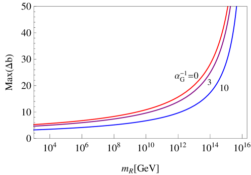
Figure 1: Maximum value of $\Delta b$ allowed by perturbativity as function of the scale $m_{R}$ in GeV. The three different lines have been calculated for three different values for the unified coupling $\alpha_{G}^{-1}$, namely $\alpha_{G}^{-1}=0,3,10$. An LR scale below 10 TeV (1 TeV) requires Max$(\Delta b_{3})\raise 1.29167pt\hbox{$\;<$\kern-7.5pt\raise-4.73611pt\hbox{$\sim\;$}}5.7$ ($5.2$) if the extreme value of $\alpha_{G}^{-1}=0$ is chosen and Max$(\Delta b_{3})\raise 1.29167pt\hbox{$\;<$\kern-7.5pt\raise-4.73611pt\hbox{$\sim\;$}}5.1$ ($4.7$) for $\alpha_{G}^{-1}=3$.

All together these considerations result in the following constraints on the allowed values for the $\Delta b^{LR}_{i}$:

$$\Delta b^{LR}_{2}=\Delta b^{LR}_{3}=\Delta b \leq 5,$$ (7)

$$\Delta b_{B-L}^{LR}+\frac{3}{2}\Delta b^{LR}_{R}-9=\frac{5}{2}\Delta b \leq \frac{25}{2}.$$

Given eq. (7) one can calculate all allowed variants of sets of $\Delta b^{LR}_{i}$, guaranteed to give GCU. Two examples are shown in fig.  2. The figure shows the running of the inverse gauge couplings as a function of the energy scale, for an assumed value of $m_{R}=10$ TeV and a SUSY scale of 1 TeV, for ($\Delta b^{LR}_{3},\Delta b^{LR}_{2},\Delta b^{LR}_{R},\Delta b^{LR}_{B-L}$) $=(0,0,1,15/2)$ (left) and $=(4,4,10,4)$ (right). The example on the left has $\alpha_{G}^{-1}\simeq 25$ as in the MSSM, while the example on the right has $\alpha_{G}^{-1}\simeq 6$. Note that while both examples lead by construction to the same value of $\alpha_{1}(m_{Z})$, they have very different values for $\alpha_{R}(m_{R})$ and $\alpha_{B-L}(m_{R})$ and thus predict different couplings for the gauge bosons $W_{R}$ and $Z^{\prime}$ of the extended gauge group.

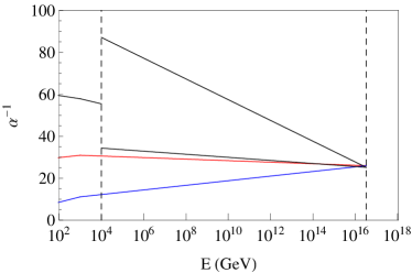
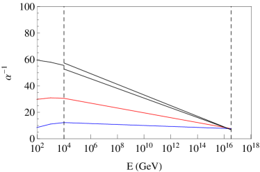
Figure 2: Gauge coupling unification in LR models for $m_{R}=10^{4}$ GeV. Left panel is for ($\Delta b^{LR}_{3},\Delta b^{LR}_{2},\Delta b^{LR}_{R},\Delta b^{LR}_{B-L}$) $=(0,0,1,15/2)$ and right panel for $(4,4,10,4)$.

With the constraints from eq. (7), we find that a total of 65 different variants can be constructed. However, after imposing that at least one of the fields that breaks correctly the $SU(2)_{R}\times U(1)_{B-L}$ symmetry to $U(1)_{Y}$ is present, either a $\Phi_{1,1,3,-2}$ or a $\Phi_{1,1,2,-1}$ (and/or their conjugates), the number of variants is reduced to 53. We list them in tables 1 and 2, together with one example of field configurations which give the corresponding $\Delta b^{LR}_{i}$.

$(\Delta b,\Delta b_{R})$	Sample field combination
(0, 1)	$\bar{\Phi}_{1,1,2,-1}+2\bar{\Phi}_{1,1,1,2}+\Phi_{1,1,2,-1}+2\Phi_{1,1,1,2}$
(0, 2)	$2\bar{\Phi}_{1,1,2,-1}+\bar{\Phi}_{1,1,1,2}+2\Phi_{1,1,2,-1}+\Phi_{1,1,1,2}$
(0, 3)	$\bar{\Phi}_{1,1,2,-1}+\bar{\Phi}_{1,1,1,2}+\Phi_{1,1,2,-1}+\Phi_{1,1,3,0}+\Phi_{1,1,1,2}$
(0, 4)	$2\bar{\Phi}_{1,1,2,-1}+2\Phi_{1,1,2,-1}+\Phi_{1,1,3,0}$
(0, 5)	$\bar{\Phi}_{1,1,2,-1}+\Phi_{1,1,2,-1}+2\Phi_{1,1,3,0}$
(1, 1)	$\bar{\Phi}_{1,2,1,1}+\bar{\Phi}_{1,1,2,-1}+2\bar{\Phi}_{1,1,1,2}+\bar{\Phi}_{3,1,1,-\frac{2}{3}}+\Phi_{1,2,1,1}+\Phi_{1,1,2,-1}+2\Phi_{1,1,1,2}+\Phi_{3,1,1,-\frac{2}{3}}$
(1, 2)	$\bar{\Phi}_{1,1,2,-1}+2\bar{\Phi}_{1,1,1,2}+\bar{\Phi}_{3,1,1,-\frac{2}{3}}+\Phi_{1,1,2,-1}+\Phi_{1,2,2,0}+2\Phi_{1,1,1,2}+\Phi_{3,1,1,-\frac{2}{3}}$
(1, 3)	$2\bar{\Phi}_{1,1,2,-1}+\bar{\Phi}_{1,1,1,2}+\bar{\Phi}_{3,1,1,-\frac{2}{3}}+2\Phi_{1,1,2,-1}+\Phi_{1,2,2,0}+\Phi_{1,1,1,2}+\Phi_{3,1,1,-\frac{2}{3}}$
(1, 4)	$\bar{\Phi}_{1,1,2,-1}+\bar{\Phi}_{1,1,1,2}+\bar{\Phi}_{3,1,1,-\frac{2}{3}}+\Phi_{1,1,2,-1}+\Phi_{1,1,3,0}+\Phi_{1,2,2,0}+\Phi_{1,1,1,2}+\Phi_{3,1,1,-\frac{2}{3}}$
(1, 5)	$2\bar{\Phi}_{1,1,2,-1}+\bar{\Phi}_{3,1,1,-\frac{2}{3}}+2\Phi_{1,1,2,-1}+\Phi_{1,1,3,0}+\Phi_{1,2,2,0}+\Phi_{3,1,1,-\frac{2}{3}}$
(1, 6)	$\bar{\Phi}_{1,1,2,-1}+\bar{\Phi}_{3,1,1,-\frac{2}{3}}+\Phi_{1,1,2,-1}+2\Phi_{1,1,3,0}+\Phi_{1,2,2,0}+\Phi_{3,1,1,-\frac{2}{3}}$
(2, 1)	$\bar{\Phi}_{1,1,2,-1}+3\bar{\Phi}_{1,1,1,2}+2\bar{\Phi}_{3,1,1,-\frac{2}{3}}+\Phi_{1,1,2,-1}+\Phi_{1,3,1,0}+3\Phi_{1,1,1,2}+2\Phi_{3,1,1,-\frac{2}{3}}$
(2, 2)	$2\bar{\Phi}_{1,1,2,-1}+2\bar{\Phi}_{1,1,1,2}+2\bar{\Phi}_{3,1,1,-\frac{2}{3}}+2\Phi_{1,1,2,-1}+\Phi_{1,3,1,0}+2\Phi_{1,1,1,2}+2\Phi_{3,1,1,-\frac{2}{3}}$
(2, 3)	$\bar{\Phi}_{1,1,2,-1}+2\bar{\Phi}_{1,1,1,2}+2\bar{\Phi}_{3,1,1,-\frac{2}{3}}+\Phi_{1,1,2,-1}+2\Phi_{1,2,2,0}+2\Phi_{1,1,1,2}+2\Phi_{3,1,1,-\frac{2}{3}}$
(2, 4)	$2\bar{\Phi}_{1,1,2,-1}+\bar{\Phi}_{1,1,1,2}+2\bar{\Phi}_{3,1,1,-\frac{2}{3}}+2\Phi_{1,1,2,-1}+2\Phi_{1,2,2,0}+\Phi_{1,1,1,2}+2\Phi_{3,1,1,-\frac{2}{3}}$
(2, 5)	$\bar{\Phi}_{1,1,2,-1}+\bar{\Phi}_{1,1,1-2}+2\bar{\Phi}_{3,1,1,-\frac{2}{3}}+\Phi_{1,1,2,-1}+\Phi_{1,1,3,0}+2\Phi_{1,2,2,0}+\Phi_{1,1,1,2}+2\Phi_{3,1,1,-\frac{2}{3}}$
(2, 6)	$2\bar{\Phi}_{1,1,2,-1}+2\bar{\Phi}_{3,1,1,-\frac{2}{3}}+2\Phi_{1,1,2,-1}+\Phi_{1,1,3,0}+2\Phi_{1,2,2,0}+2\Phi_{3,1,1,-\frac{2}{3}}$
(2, 7)	$\bar{\Phi}_{1,1,2,-1}+2\bar{\Phi}_{3,1,1,-\frac{2}{3}}+\Phi_{1,1,2,-1}+2\Phi_{1,1,3,0}+2\Phi_{1,2,2,0}+2\Phi_{3,1,1,-\frac{2}{3}}$
(2, 8)	$\bar{\Phi}_{1,1,2,-1}+\bar{\Phi}_{3,1,2,\frac{1}{3}}+\Phi_{1,1,2,-1}+\Phi_{1,1,3,0}+2\Phi_{1,2,2,0}+\Phi_{3,1,2,\frac{1}{3}}$
(3, 1)	$\bar{\Phi}_{1,2,1,1}+\bar{\Phi}_{1,1,2,-1}+4\bar{\Phi}_{1,1,1,2}+\Phi_{1,2,1,1}+\Phi_{1,1,2,-1}+\Phi_{1,3,1,0}+\Phi_{8,1,1,0}+4\Phi_{1,1,1,2}$
(3, 2)	$\bar{\Phi}_{1,1,2,-1}+4\bar{\Phi}_{1,1,1,2}+\Phi_{1,1,2,-1}+\Phi_{1,3,1,0}+\Phi_{1,2,2,0}+\Phi_{8,1,1,0}+4\Phi_{1,1,1,2}$
(3, 3)	$2\bar{\Phi}_{1,1,2,-1}+3\bar{\Phi}_{1,1,1,2}+2\Phi_{1,1,2,-1}+\Phi_{1,3,1,0}+\Phi_{1,2,2,0}+\Phi_{8,1,1,0}+3\Phi_{1,1,1,2}$
(3, 4)	$\bar{\Phi}_{1,2,1,1}+\bar{\Phi}_{1,1,3,-2}+\Phi_{1,2,1,1}+\Phi_{1,3,1,0}+\Phi_{8,1,1,0}+\Phi_{1,1,3,-2}$
(3, 5)	$\bar{\Phi}_{1,1,3,-2}+\Phi_{1,3,1,0}+\Phi_{1,2,2,0}+\Phi_{8,1,1,0}+\Phi_{1,1,3,-2}$
(3, 6)	$\bar{\Phi}_{1,1,2,-1}+2\bar{\Phi}_{1,1,1,2}+\Phi_{1,1,2,-1}+\Phi_{1,1,3,0}+3\Phi_{1,2,2,0}+\Phi_{8,1,1,0}+2\Phi_{1,1,1,2}$
(3, 7)	$2\bar{\Phi}_{1,1,2,-1}+\bar{\Phi}_{1,1,1-2}+2\Phi_{1,1,2,-1}+\Phi_{1,1,3,0}+3\Phi_{1,2,2,0}+\Phi_{8,1,1,0}+\Phi_{1,1,1,2}$
(3, 8)	$\bar{\Phi}_{1,1,2,-1}+\bar{\Phi}_{1,1,1,2}+\Phi_{1,1,2,-1}+2\Phi_{1,1,3,0}+3\Phi_{1,2,2,0}+\Phi_{8,1,1,0}+\Phi_{1,1,1,2}$
(3, 9)	$2\bar{\Phi}_{1,1,2,-1}+2\Phi_{1,1,2,-1}+2\Phi_{1,1,3,0}+3\Phi_{1,2,2,0}+\Phi_{8,1,1,0}$
(3, 10)	$\bar{\Phi}_{1,1,2,-1}+\Phi_{1,1,2,-1}+3\Phi_{1,1,3,0}+3\Phi_{1,2,2,0}+\Phi_{8,1,1,0}$

Table 1: List of the 53 variants with a single LR scale. Shown are the 29 variants with $\Delta b_{3}<4$. In each case, the fields shown are the extra ones which are needed besides the ones contained in the MSSM representations (the 2 Higgs doublets are assumed to come from one bi-doublet $\Phi_{1,2,2,0}$). The $\Delta b_{3},\Delta b_{2},\Delta b_{R},\Delta b_{B-L}$ values can be obtained from the first column through eqs (7).

$(\Delta b,\Delta b_{R})$	Sample field combination
(4, 1)	$\bar{\Phi}_{1,1,2,-1}+5\bar{\Phi}_{1,1,1,2}+\bar{\Phi}_{3,1,1,-\frac{2}{3}}+\Phi_{1,1,2,-1}+2\Phi_{1,3,1,0}+\Phi_{8,1,1,0}+5\Phi_{1,1,1,2}+\Phi_{3,1,1,-\frac{2}{3}}$
(4, 2)	$2\bar{\Phi}_{1,1,2,-1}+4\bar{\Phi}_{1,1,1,2}+\bar{\Phi}_{3,1,1,-\frac{2}{3}}+2\Phi_{1,1,2,-1}+2\Phi_{1,3,1,0}+\Phi_{8,1,1,0}+4\Phi_{1,1,1,2}+\Phi_{3,1,1,-\frac{2}{3}}$
(4, 3)	$\bar{\Phi}_{1,1,2,-1}+4\bar{\Phi}_{1,1,1,2}+\bar{\Phi}_{3,1,1,-\frac{2}{3}}+\Phi_{1,1,2,-1}+\Phi_{1,3,1,0}+2\Phi_{1,2,2,0}+\Phi_{8,1,1,0}+4\Phi_{1,1,1,2}+\Phi_{3,1,1,-\frac{2}{3}}$
(4, 4)	$\bar{\Phi}_{1,1,1,2}+\bar{\Phi}_{3,1,1,-\frac{2}{3}}+\bar{\Phi}_{1,1,3,-2}+2\Phi_{1,3,1,0}+\Phi_{8,1,1,0}+\Phi_{1,1,1,2}+\Phi_{3,1,1,-\frac{2}{3}}+\Phi_{1,1,3,-2}$
(4, 5)	$\bar{\Phi}_{1,1,2,-1}+\bar{\Phi}_{3,1,1,-\frac{2}{3}}+\bar{\Phi}_{1,1,3,-2}+\Phi_{1,1,2,-1}+2\Phi_{1,3,1,0}+\Phi_{8,1,1,0}+\Phi_{3,1,1,-\frac{2}{3}}+\Phi_{1,1,3,-2}$
(4, 6)	$\bar{\Phi}_{3,1,1,-\frac{2}{3}}+\bar{\Phi}_{1,1,3,-2}+\Phi_{1,3,1,0}+2\Phi_{1,2,2,0}+\Phi_{8,1,1,0}+\Phi_{3,1,1,-\frac{2}{3}}+\Phi_{1,1,3,-2}$
(4, 7)	$\bar{\Phi}_{1,1,2,-1}+2\bar{\Phi}_{1,1,1,2}+\bar{\Phi}_{3,1,1,-\frac{2}{3}}+\Phi_{1,1,2,-1}+\Phi_{1,1,3,0}+4\Phi_{1,2,2,0}+\Phi_{8,1,1,0}+2\Phi_{1,1,1,2}+\Phi_{3,1,1,-\frac{2}{3}}$
(4, 8)	$2\bar{\Phi}_{1,1,2,-1}+\bar{\Phi}_{1,1,1,2}+\bar{\Phi}_{3,1,1,-\frac{2}{3}}+2\Phi_{1,1,2,-1}+\Phi_{1,1,3,0}+4\Phi_{1,2,2,0}+\Phi_{8,1,1,0}+\Phi_{1,1,1,2}+\Phi_{3,1,1,-\frac{2}{3}}$
(4, 9)	$\bar{\Phi}_{1,1,2,-1}+\bar{\Phi}_{1,1,1,2}+\bar{\Phi}_{3,1,1,-\frac{2}{3}}+\Phi_{1,1,2,-1}+2\Phi_{1,1,3,0}+4\Phi_{1,2,2,0}+\Phi_{8,1,1,0}+\Phi_{1,1,1,2}+\Phi_{3,1,1,-\frac{2}{3}}$
(4, 10)	$2\bar{\Phi}_{1,1,2,-1}+\bar{\Phi}_{3,1,1,-\frac{2}{3}}+2\Phi_{1,1,2,-1}+2\Phi_{1,1,3,0}+4\Phi_{1,2,2,0}+\Phi_{8,1,1,0}+\Phi_{3,1,1,-\frac{2}{3}}$
(4, 11)	$\bar{\Phi}_{1,1,2,-1}+\bar{\Phi}_{3,1,1,-\frac{2}{3}}+\Phi_{1,1,2,-1}+3\Phi_{1,1,3,0}+4\Phi_{1,2,2,0}+\Phi_{8,1,1,0}+\Phi_{3,1,1,-\frac{2}{3}}$
(5, 1)	$\bar{\Phi}_{1,2,1,1}+\bar{\Phi}_{1,1,2,-1}+5\bar{\Phi}_{1,1,1,2}+2\bar{\Phi}_{3,1,1,-\frac{2}{3}}+\Phi_{1,2,1,1}+\Phi_{1,1,2,-1}+2\Phi_{1,3,1,0}+\Phi_{8,1,1,0}$
	$+5\Phi_{1,1,1,2}+2\Phi_{3,1,1,-\frac{2}{3}}$
(5, 2)	$\bar{\Phi}_{1,1,2,-1}+5\bar{\Phi}_{1,1,1,2}+2\bar{\Phi}_{3,1,1,-\frac{2}{3}}+\Phi_{1,1,2,-1}+2\Phi_{1,3,1,0}+\Phi_{1,2,2,0}+\Phi_{8,1,1,0}+5\Phi_{1,1,1,2}$
	$+2\Phi_{3,1,1,-\frac{2}{3}}$
(5, 3)	$2\bar{\Phi}_{1,1,2,-1}+4\bar{\Phi}_{1,1,1,2}+2\bar{\Phi}_{3,1,1,-\frac{2}{3}}+2\Phi_{1,1,2,-1}+2\Phi_{1,3,1,0}+\Phi_{1,2,2,0}+\Phi_{8,1,1,0}+4\Phi_{1,1,1,2}$
	$+2\Phi_{3,1,1,-\frac{2}{3}}$
(5, 4)	$\bar{\Phi}_{1,2,1,1}+\bar{\Phi}_{1,1,1,2}+2\bar{\Phi}_{3,1,1,-\frac{2}{3}}+\bar{\Phi}_{1,1,3,-2}+\Phi_{1,2,1,1}+2\Phi_{1,3,1,0}+\Phi_{8,1,1,0}+\Phi_{1,1,1,2}+2\Phi_{3,1,1,-\frac{2}{3}}$
	$+\Phi_{1,1,3,-2}$
(5, 5)	$\bar{\Phi}_{1,1,1,2}+2\bar{\Phi}_{3,1,1,-\frac{2}{3}}+\bar{\Phi}_{1,1,3,-2}+2\Phi_{1,3,1,0}+\Phi_{1,2,2,0}+\Phi_{8,1,1,0}+\Phi_{1,1,1,2}+2\Phi_{3,1,1,-\frac{2}{3}}$
	$+\Phi_{1,1,3,-2}$
(5, 6)	$\bar{\Phi}_{1,1,2,-1}+2\bar{\Phi}_{3,1,1,-\frac{2}{3}}+\bar{\Phi}_{1,1,3,-2}+\Phi_{1,1,2,-1}+2\Phi_{1,3,1,0}+\Phi_{1,2,2,0}+\Phi_{8,1,1,0}+2\Phi_{3,1,1,-\frac{2}{3}}$
	$+\Phi_{1,1,3,-2}$
(5, 7)	$2\bar{\Phi}_{3,1,1,-\frac{2}{3}}+\bar{\Phi}_{1,1,3,-2}+\Phi_{1,3,1,0}+3\Phi_{1,2,2,0}+\Phi_{8,1,1,0}+2\Phi_{3,1,1,-\frac{2}{3}}+\Phi_{1,1,3,-2}$
(5, 8)	$\bar{\Phi}_{3,1,2,\frac{1}{3}}+\bar{\Phi}_{1,1,3,-2}+2\Phi_{1,3,1,0}+\Phi_{1,2,2,0}+\Phi_{8,1,1,0}+\Phi_{3,1,2,\frac{1}{3}}+\Phi_{1,1,3,-2}$
(5, 9)	$2\bar{\Phi}_{1,1,2,-1}+\bar{\Phi}_{1,1,1,2}+2\bar{\Phi}_{3,1,1,-\frac{2}{3}}+2\Phi_{1,1,2,-1}+\Phi_{1,1,3,0}+5\Phi_{1,2,2,0}+\Phi_{8,1,1,0}+\Phi_{1,1,1,2}$
	$+2\Phi_{3,1,1,-\frac{2}{3}}$
(5, 10)	$\bar{\Phi}_{1,1,2,-1}+\bar{\Phi}_{1,1,1,2}+2\bar{\Phi}_{3,1,1,-\frac{2}{3}}+\Phi_{1,1,2,-1}+2\Phi_{1,1,3,0}+5\Phi_{1,2,2,0}+\Phi_{8,1,1,0}+\Phi_{1,1,1,2}$
	$+2\Phi_{3,1,1,-\frac{2}{3}}$
(5, 11)	$2\bar{\Phi}_{1,1,2,-1}+2\bar{\Phi}_{3,1,1,-\frac{2}{3}}+2\Phi_{1,1,2,-1}+2\Phi_{1,1,3,0}+5\Phi_{1,2,2,0}+\Phi_{8,1,1,0}+2\Phi_{3,1,1,-\frac{2}{3}}$
(5, 12)	$\bar{\Phi}_{1,1,2,-1}+2\bar{\Phi}_{3,1,1,-\frac{2}{3}}+\Phi_{1,1,2,-1}+3\Phi_{1,1,3,0}+5\Phi_{1,2,2,0}+\Phi_{8,1,1,0}+2\Phi_{3,1,1,-\frac{2}{3}}$
(5, 13)	$\bar{\Phi}_{1,1,2,-1}+\bar{\Phi}_{3,1,2,\frac{1}{3}}+\Phi_{1,1,2,-1}+2\Phi_{1,1,3,0}+5\Phi_{1,2,2,0}+\Phi_{8,1,1,0}+\Phi_{3,1,2,\frac{1}{3}}$

Table 2: List of the 53 variants with a single LR scale. Shown are the remaining 24 variants, with $\Delta b_{3}\geq 4$.

We give only one example for each configuration in tables 1 and 2, although we went through the exercise of finding all possible configurations for the 53 variants with the field content of table 4. In total there are 5324 anomaly-free configurations wp . Only the variants (0,1), (0,2), (0,4) and (0,5) have only one configuration, while larger numbers of configurations are usually found for larger values of $\Delta b^{LR}_{3}$.

Not all the fields in table 4 can lead to valid configurations. The fields which never give an anomaly-free configuration are: $\Phi_{8,2,2,0}$, $\Phi_{3,2,2,\frac{4}{3}}$, $\Phi_{3,3,1,-\frac{2}{3}}$, $\Phi_{3,1,3,-\frac{2}{3}}$, $\Phi_{6,3,1,\frac{2}{3}}$, $\Phi_{6,1,3,\frac{2}{3}}$ and $\Phi_{1,3,3,0}$. Also the field $\Phi_{3,2,2,-\frac{2}{3}}$ appears only exactly once in the variant (5,5) in the configuration $4\Phi_{1,2,1,1}+\Phi_{3,1,1,-\frac{2}{3}}+\Phi_{3,2,2,-\frac{2}{3}}+4\Phi_{1,1,2,1}+2\Phi_{1,1,1,2}+5\Phi_{3,1,1,-\frac{2}{3}}$. Note that, the example configurations we give for the variants (1,3) and (1,4) are not the model-II and model-I discussed in DeRomeri:2011ie .

Many of the 53 variants have only configurations with $\Phi_{1,1,2,-1}$ (and conjugate) for the breaking of the LR-symmetry. These variants need either the presence of $\Phi_{1,3,1,0}$ [as for example in the configuration shown for variant (2,1)] or $\Phi_{1,1,3,0}$ [see, for example (1,4)] or an additional singlet $\Phi_{1,1,1,0}$ (not shown, since no contribution to any $\Delta b^{LR}_{i}$), to generate seesaw neutrino masses. Using the $\Phi_{1,1,1,0}$ one could construct either an inverse mohapatra:1986bd or a linear Akhmedov:1995ip ; Akhmedov:1995vm seesaw mechanism, while with $\Phi_{1,3,1,0}$ a seesaw type-III Foot:1988aq is a possibility and, finally a $\Phi_{1,1,3,0}$ allows for an inverse seesaw type-III DeRomeri:2011ie . The first example where a valid configuration with $\Phi_{1,1,3,-2}$ appears is the variant (3,4). The simplest configuration is $\Phi_{1,2,1,1}+\Phi_{1,3,1,0}+\Phi_{8,1,1,0}+\Phi_{1,1,3,-2}+{\bar{\Phi}_{1,2,1,1}}+{\bar{\Phi}_{1,1,3,-2}}$ (not the example given in table 1). The vev of the $\Phi_{1,1,3,-2}$ does not only break the LR symmetry, it can also generate a Majorana mass term for the right-handed neutrino fields, i.e. configurations with $\Phi_{1,1,3,-2}$ can generate a seesaw type-I, in principle. Finally, the simplest possibility with a valid configuration including $\Phi_{1,3,1,-2}$ is found in variant (4,1) with $\Phi_{1,1,2,-1}+\Phi_{8,1,1,0}+\Phi_{1,1,1,2}+\Phi_{3,1,1,\frac{4}{3}}+\Phi_{1,3,1,-2}+\bar{\Phi}_{1,1,2,-1}+\bar{\Phi}_{1,1,1,2}+\bar{\Phi}_{3,1,1,\frac{4}{3}}+\bar{\Phi}_{1,3,1,-2}$. The presence of $\Phi_{1,3,1,-2}$ allows to generate a seesaw type-II for the neutrinos.

As mentioned in the introduction, it is not possible to construct a sliding scale model in which the LR symmetry is broken by two pairs of triplets: $\Phi_{1,3,1,-2}+\bar{\Phi}_{1,3,1,-2}+\Phi_{1,1,3,-2}+\bar{\Phi}_{1,1,3,-2}$. The sum of the $\Delta b$’s for these fields adds up to $(\Delta b^{LR}_{3},b^{LR}_{L},\Delta b^{LR}_{R},\Delta b^{LR}_{B-L})=(0,4,4,18)$. This leaves only the possibilities ($4,4$), ($5,4$), ($5,5$), etc. from table 2. However, the largest $\Delta b^{LR}_{B-L}$ of these models is ($5,4$) which allows for $\Delta b^{LR}_{B-L}=31/2$, smaller than the required 18. This observation is consistent with the analysis done in Majee:2007uv , where the authors have shown that a supersymmetric LR-symmetric model, where the LR symmetry is broken by two pairs of triplets, requires a minimal LR scale of at least $10^{9}$ GeV (and, actually, a much larger scale in minimal renormalizable models, if GUT scale thresholds are small).

A few final comments on the variants with $\Delta b^{LR}_{2}=\Delta b^{LR}_{3}=0$. Strictly speaking, none of these variants is guaranteed to give a valid model in the sense defined in sub-section II.1, since they contain only one $\Phi_{1,2,2,0}\rightarrow(H_{u},H_{d})$ and no vector-like quarks (no $\Phi_{3,1,1,\frac{4}{3}}$ or $\Phi_{3,1,1,-\frac{2}{3}}$). With such a minimal configuration the CKM matrix is trivial at the energy scale where the LR symmetry is broken. We nevertheless list these variants, since in principle a CKM matrix for quarks consistent with experimental data could be generated at 1-loop level from flavor violating soft terms, as discussed in Babu:1998tm .

Before we end this section let us mention that variants with $\Delta b_{3}^{LR}=5$ will not be testable at LHC by measurements of soft SUSY breaking mass terms (“invariants”). This is discussed below in section III.1.

II.3 Model class-II: Additional intermediate Pati-Salam scale

In the second class of supersymmetric $SO(10)$ models we consider, $SO(10)$ is broken first to the Pati-Salam (PS) group. The complete breaking chain thus is:

$$SO(10) \to SU(4)\times SU(2)_{L}\times SU(2)_{R}$$

$$\to SU(3)_{c}\times SU(2)_{L}\times SU(2)_{R}\times U(1)_{B-L}\to\hskip 5.69054pt{\rm MSSM}\textrm{.}$$

The representations available from the decomposition of $SO(10)$ multiplets up to ${\bf 126}$ are listed in table 5 in the appendix, together with their possible $SO(10)$ origin. Breaking $SO(10)$ to the PS group requires that $\Psi_{1,1,1}$ from the ${\bf 54}$ takes a vev. The subsequent breaking of the PS group to the LR group requires that the singlet in $\Psi_{15,1,1}$, originally from the ${\bf 45}$ of $SO(10)$, acquires a vev. And, finally, as before in the LR-class, the breaking of LR to $SU(3)_{c}\times SU(2)_{L}\times U(1)_{Y}$ can be either done via $\Phi_{1,1,2,-1}$ or $\Phi_{1,1,3,-2}$ (and/or conjugates).

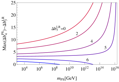
Figure 3: Maximum value of $\Delta b^{PS}_{4}-\Delta b^{LR}_{3}$ allowed by perturbativity as function of the scale $m_{PS}$ in GeV. The different lines have been calculated for six different values of $\Delta b^{LR}_{3}$. The plot assumes that $m_{R}=1$ TeV. The line near the bottom corresponds to $\Delta b_{3}^{LR}=7$.

The additional $b_{i}$ coefficients for the regime $[m_{PS},m_{GUT}]$ are given by:

$$(b_{4}^{PS},b_{2}^{PS},b_{R}^{PS}) =(-6,1,1)+(\Delta b_{4}^{PS},\Delta b_{2}^{PS},\Delta b_{R}^{PS})$$ (9)

where, as before, the $\Delta b_{i}^{PS}$ include contributions from superfields not part of the MSSM field content.

In this class of models, the unification scale is independent of the LR one if the following condition is satisfied:

$$0= \begin{pmatrix}\Delta b_{3}^{LR}-\Delta b_{2}^{LR},&\frac{3}{5}\Delta b_{R}^{LR}+\frac{2}{5}\Delta b_{B-L}^{LR}-\Delta b_{2}^{LR}-\frac{18}{5}\end{pmatrix}.\begin{pmatrix}\begin{array}[]{rr}2&3\\ -5&0\end{array}\end{pmatrix}.\begin{pmatrix}\Delta b_{4}^{PS}-\Delta b_{2}^{PS}-3\\ \Delta b_{R}^{PS}-\Delta b_{2}^{PS}-12\end{pmatrix}$$ (10)

It is worth noting that requiring also that $m_{PS}$ is independent of the LR scale would lead to the conditions in eq. (7), which are the sliding conditions for LR models. We can see that this must be so in the following way: for some starting values at $m_{PS}$ of the three gauge couplings, the scales $m_{PS}$ and $m_{G}$ can be adjusted such that the two splittings between the three gauge couplings are reduced to zero at $m_{G}$. This fixes these scales, which must not change even if $m_{R}$ is varied. As such $\alpha_{3}^{-1}\left(m_{PS}\right)-\alpha_{2}^{-1}\left(m_{PS}\right)$ and $\alpha_{3}^{-1}\left(m_{PS}\right)-\alpha_{R}^{-1}\left(m_{PS}\right)$ are also fixed and they can be determined by running the MSSM up to $m_{PS}$. The situation is therefore equal to the one that lead to the equalities in eq. (7), namely the splittings between the gauge couplings at some fixed scale must be independent of $m_{R}$.

Since there are now two unknown scales involved in the problem, the maximum $\Delta b^{X}_{i}$ allowed by perturbativity in one regime do not only depend on the new scale $X$, but also on the $\Delta b^{Y}_{i}$ in the other regime as well. As an example, in fig.  3 we show the Max($\Delta b^{PS}_{4}$) allowed by $\alpha_{G}^{-1}\geq 0$ for different values of $\Delta b^{LR}_{3}$ and for the choice $m_{R}=1$ TeV and and $m_{G}=10^{16}$ GeV. The dependence of Max($\Delta b^{PS}_{4}$) on $m_{R}$ is rather weak, as long as $m_{R}$ does not approach the GUT scale.

If we impose the limits $m_{R}=10^{3}$ GeV, $m_{PS}\leq 10^{6}$ GeV and take $m_{G}=10^{16}$ GeV, the bounds for the different $\Delta b^{{}^{\prime}}s$ can be written as:

$$\Delta b_{2}^{PS}+\frac{3}{10}\Delta b_{2}^{LR} <7.2$$ (11)

$$\Delta b_{4}^{PS}+\frac{3}{10}\Delta b_{3}^{LR} <10$$ (12)

$$\frac{2}{5}\Delta b_{4}^{PS}+\frac{3}{5}\Delta b_{R}^{PS}+\frac{3}{10}\left(\frac{2}{5}\Delta b_{B-L}^{LR}+\frac{3}{5}\Delta b_{R}^{LR}\right) <17$$ (13)

However, as fig.  (3) shows, Max($\Delta b^{PS}_{4}$) is a rather strong function of the choice of $\Delta b^{LR}_{3}$. Note, that if $m_{PS}$ is low, say below $10^{10}$ GeV larger $\Delta b^{LR}_{3}$ are possible, up to $\Delta b^{LR}_{3}=7$, see fig. (3). The large values of Max($\Delta b^{LR}$) and Max($\Delta b^{PS}$) allow, in principle, a huge number of variants to be constructed in class-II. This is demonstrated in fig.  (4), where we show the number of variants for an assumed $m_{R}\sim 1$ TeV as a function of the scale $m_{PS}$. Up to $m_{PS}=10^{15}$ GeV the list is exhaustive. For larger values of $m_{PS}$ we have only scanned a finite (though large) set of possible variants. Note, that these are variants, not configurations. As in the case of class-I practically any variant can be made by several possible anomaly-free configurations. The exhaustive list of variants ($m_{PS}=10^{15}$ GeV) contains a total of 105909 possibilities and can be found in wp .

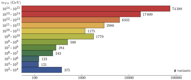
Figure 4: The number of possible variants in model class-II, assuming $m_{R}$ is of order $m_{R}\simeq 1$ TeV as a function of $m_{PS}$. Up to $m_{PS}=10^{15}$ GeV the list is exhaustive. For larger values of $m_{PS}$ we have only scanned a finite (though large) set of possible variants.

With such a huge number of possible variants, we can discuss only some general features here. First of all, within the exhaustive set up to $m_{PS}=10^{15}$ GeV, there are a total of 1570 different sets of $\Delta b^{LR}_{i}$, each of which can be completed by more than one set of $\Delta b^{PS}_{i}$. Variants with the same set of $\Delta b^{LR}_{i}$ but different completion of $\Delta b^{PS}_{i}$ have, of course, the same configuration in the LR-regime, but come with a different value for $m_{PS}$ for fixed $m_{R}$. Thus, they have in general different values for $\alpha_{B-L}$ and $\alpha_{R}$ at the LR scale and, see next section, different values of the invariants. For example, for the smallest values of $\Delta b^{LR}_{i}$, that are possible in principle [$\Delta b^{LR}_{i}=(0,0,1,3/2)$], there are 342 different completing sets of $\Delta b^{PS}_{i}$.

The very simplest set of $\Delta b^{LR}_{i}$ possible, $\Delta b^{LR}_{i}=(0,0,1,3/2)$, corresponds to the configuration $\Phi_{1,1,2,-1}+\bar{\Phi}_{1,1,2,-1}$. These fields are necessary to break $SU(2)_{R}\times U(1)_{B-L}\to U(1)_{Y}$. Their presence in the LR regime requires that in the PS-regime we have at least one set of copies of $\Psi_{4,1,2}+\bar{\Psi}_{4,1,2}$. In addition, for breaking the PS group to the LR group, we need at least one copy of $\Psi_{15,1,1}$. However, the set of $\Psi_{4,1,2}+\bar{\Psi}_{4,1,2}+\Psi_{15,1,1}$ is not sufficient to generate a sliding scale mechanism and the simplest configuration that can do so, consistent with $\Delta b^{LR}_{i}=(0,0,1,3/2)$, is $3\Psi_{1,2,2}+4\Psi_{1,1,3}+\Psi_{4,1,2}+\bar{\Psi}_{4,1,2}+\Psi_{15,1,1}$, leading to $\Delta b^{PS}_{i}=(6,3,15)$ and a very low possible value of $m_{PS}$ of $m_{PS}=8.2$ TeV for $m_{R}=1$ TeV (see, however, the discussion on leptoquarks below). The next possible completion for $\Phi_{1,1,2,-1}+\bar{\Phi}_{1,1,2,-1}$ is $3\Psi_{1,2,2}+5\Psi_{1,1,3}+\Psi_{4,1,2}+\bar{\Psi}_{4,1,2}+\Psi_{15,1,1}$, with $\Delta b^{PS}_{i}=(6,3,17)$ and $m_{PS}=1.3\times 10^{8}$ GeV (for $m_{R}=1$ TeV), etc.

As noted already in section II.2, one copy of $\Phi_{1,2,2,0}$ is not sufficient to produce a realistic CKM matrix at tree-level. Thus, the minimal configuration of $\Phi_{1,1,2,-1}+\bar{\Phi}_{1,1,2,-1}$ relies on the possibility of generating all of the departure of the CKM matrix from unity by flavor violating soft masses Babu:1998tm . There are at least two possibilities to generate a non-trivial CKM at tree-level, either by adding (a) another $\Phi_{1,2,2,0}$ plus (at least) one copy of $\Phi_{1,1,3,0}$ or via (b) one copy of “vector-like quarks” $\Phi_{3,1,1,\frac{4}{3}}$ or $\Phi_{3,1,1,-\frac{2}{3}}$. Consider the configuration $\Phi_{1,1,2,-1}+\bar{\Phi}_{1,1,2,-1}+\Phi_{1,2,2,0}+\Phi_{1,1,3,0}$ first. It leads to $\Delta b^{LR}_{i}=(0,1,4,3/2)$. Since $\Phi_{1,2,2,0}$ and $\Phi_{1,1,3,0}$ must come from $\Psi_{1,2,2}$ (or $\Psi_{15,2,2}$) and $\Psi_{1,1,3}$, respectively, the simplest completion for this set of $\Delta b^{LR}_{i}$ is again $3\Psi_{1,2,2}+4\Psi_{1,1,3}+\Psi_{4,1,2}+\bar{\Psi}_{4,1,2}+\Psi_{15,1,1}$, leading to $\Delta b^{PS}_{i}=(6,3,15)$ and value of $m_{PS}$ of, in this case, $m_{PS}=5.4$ TeV for $m_{R}=1$ TeV. Again, many completions with different $\Delta b^{PS}_{i}$ exist for this set of $\Delta b^{LR}_{i}$.

The other possibility for generating CKM at tree-level, adding for example a pair of $\Phi_{3,1,1,-\frac{2}{3}}+\bar{\Phi}_{3,1,1,-\frac{2}{3}}$, has $\Delta b^{LR}_{i}=(1,0,1,5/2)$ and its simplest PS-completion is $4\Psi_{1,2,2}+4\Psi_{1,1,3}+\Psi_{4,1,2}+\bar{\Psi}_{4,1,2}+\Psi_{6,1,1}+\Psi_{15,1,1}$, with $\Delta b^{PS}_{i}=(7,4,16)$ and a $m_{PS}=4.6\times 10^{6}$ TeV for $m_{R}=1$ TeV. Also in this case one can find sets with very low values of $m_{PS}$. For example, adding a $\Phi_{1,2,2,0}$ to this LR-configuration (for a $\Delta b^{LR}_{i}=(1,1,2,5/2)$), one finds that with the same $\Delta b^{PS}_{i}$ now a value of $m_{PS}$ as low as $m_{PS}=8.3$ TeV for $m_{R}=1$ TeV is possible.

We note in passing that the original PS-class model of DeRomeri:2011ie in our notation corresponds to $\Delta b^{LR}_{i}=(1,2,10,4)$ and $\Phi_{1,1,2,-1}+\bar{\Phi}_{1,1,2,-1}+\Phi_{1,2,1,1}+\bar{\Phi}_{1,2,1,1}+\Phi_{1,2,2,0}+4\Phi_{1,1,3,0}+\Phi_{3,1,1,-\frac{2}{3}}+\bar{\Phi}_{3,1,1,-\frac{2}{3}}$, completed by $\Delta b^{PS}_{i}=(9,5,13)$ with $\Psi_{4,1,2}+\bar{\Psi}_{4,1,2}+\Psi_{4,2,1}+\Psi_{4,2,1}+\Psi_{1,2,2}+4\Psi_{1,1,3}+\Psi_{6,1,1}+\Psi_{15,1,1}$. The lowest possible $m_{PS}$ for a $m_{R}=1$ TeV is $m_{PS}=2.4\times 10^{8}$ GeV. Obviously this example is not the simplest construction in class-II. We also mention that while for the $\beta$-coefficients it does not make any difference, the superfield $\Phi_{1,1,3,0}$ can be either interpreted as “Higgs” or as “matter”. In the original construction DeRomeri:2011ie this “arbitrariness” was used to assign the 4 copies of $\Phi_{1,1,3,0}$ to one copy of $\Omega^{c}=\Phi_{1,1,3,0}$, i.e. “Higgs” and three copies of $\Sigma^{c}=\Phi_{1,1,3,0}$, i.e. “matter”. In this way $\Omega^{c}$ can be used to generate the CKM matrix at tree-level (together with the extra bi-doublet $\Phi_{1,2,2,0}$), while the $\Sigma^{c}$ can be used to generate an inverse seesaw type-III for neutrino masses.

As fig. (4) shows, there are more than 600 variant in which $m_{PS}$ can, in principle, be lower than $m_{PS}=10^{3}$ TeV. Such low PS scales, however, are already constrained by searches for rare decays, such as $B_{s}\to\mu^{+}\mu^{-}$. This is because the $\Psi_{15,1,1}$, which must be present in all our constructions for the breaking of the PS group, contains two leptoquark states. We will not study in detail leptoquark phenomenology Davidson:1993qk here, but mention that in the recent paper Kuznetsov:2012ad absolute lower bounds on leptoquarks within PS models of the order of $m_{PS}\simeq 40$ TeV have been derived. There are 426 variants for which we find $m_{PS}$ lower than this bound, if we put $m_{R}$ to 1 TeV. Due to the sliding scale nature of our construction this, of course, does not mean that these models are ruled by the lower limit found in Kuznetsov:2012ad . Instead, for these models one can calculate a lower limit on $m_{R}$ from the requirement that $m_{PS}=40$ TeV. Depending on the model, lower limits on $m_{R}$ between $m_{R}=[1.3,27.7]$ TeV are found for the 426 variants from this requirement.

Two example solutions can be seen in fig. 5. We have chosen one example with a very low $m_{PS}$ (left) and one with an intermediate $m_{PS}$ (right). Note, that different from the class-I models, in the class-II models the GUT scale is no longer fixed to the MSSM value $m_{G}\approx 2\times 10^{16}$ GeV. Our samples are restricted to variants which have $m_{G}$ in the interval [$10^{16},10^{18}$] GeV.

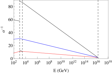
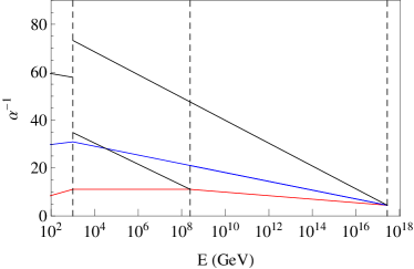
Figure 5: Gauge coupling unification for PS models with $m_{R}=10^{3}$ GeV. In the plot to the left $(\Delta b^{LR}_{3},\Delta b^{LR}_{L},\Delta b^{LR}_{R},\Delta b^{LR}_{B-L},\Delta b^{PS}_{4},\Delta b_{L}^{PS},\Delta b_{R}^{PS})=(3,5,10,3/2,8,5,17$), while the plot to the right corresponds to $\Delta b^{{}^{\prime}}s=(3,4,12,6,8,4,12)$.

II.4 Models with an $U(1)_{R}\times U(1)_{B-L}$ intermediate scale

Finally, we consider models where there is an additional intermediate symmetry $U(1)_{R}\times U(1)_{B-L}$ that follows the stage $SU(2)_{R}\times U(1)_{B-L}$. The field content relevant to this model is specified in table 6 of the appendix. In this case the original $SO(10)$ is broken down to the MSSM in three steps,

$$SO(10) \to SU(3)_{c}\times SU(2)_{L}\times SU(2)_{R}\times U(1)_{B-L}$$

$$\to SU(3)_{c}\times SU(2)_{L}\times U(1)_{R}\times U(1)_{B-L}\to\hskip 5.69054pt{\rm MSSM}\textrm{.}$$

The first step is achieved in the same way as in class-I models. The subsequent breaking $SU(2)_{R}\times U(1)_{B-L}\rightarrow U(1)_{R}\times U(1)_{B-L}$ is triggered by $\Phi_{5}=\Phi_{1,1,3,0}$ and the last one requires $\Phi_{4}^{{}^{\prime}}=\Phi^{\prime}_{1,1,\frac{1}{2},-1}$, $\Phi_{20}^{{}^{\prime}}=\Phi^{\prime}_{1,1,1,-2}$ or their conjugates.

In theories with more that one $U(1)$ gauge factor, the one loop evolution of the gauge couplings and soft-SUSY-breaking terms are affected by the extra kinetic mixing terms. The couplings are defined by the matrix

$$G=\left(\begin{array}[]{cc}g_{RR}&g_{RX}\\ g_{XR}&g_{XX}\end{array}\right).$$ (17)

and $A(t)=(GG^{T})/(4\pi)=(A^{-1}(t_{0})-\gamma(t-t_{0}))^{-1}$, where $t=\frac{1}{2\pi}\log(\frac{\mu}{\mu_{0}})$ DeRomeri:2011ie . Here, $\mu$ and $\mu_{0}$ stand for the energy scale and its normalization point and $A$ is the generalization of $\alpha$ to matrix form. The matrix of anomalous dimension, $\gamma$, is defined by the charges of each chiral superfield $f$ under $U(1)_{R}$ and $U(1)_{B-L}$:

$$\gamma=\sum_{f}Q_{f}Q_{f}^{T}$$ (18)

where $Q_{f}$ denotes a column vector of those charges. Taking the MSSM’s field content we find

$$\gamma=\left(\begin{array}[]{cc}7&0\\ 0&6\end{array}\right).$$ (21)

To ensure the canonical normalization of the $B-L$ charge within the $SO(10)$ framework, $\gamma$ should be normalized as $\gamma^{can}=N\gamma^{phys}N$, where $N=\text{diag}(1,\sqrt{3/8})$.

Then, the additional $\beta$ coefficients for the running step $[m_{B-L},m_{R}]$ are given by,

$$(b_{3}^{B-L},b_{2}^{B-L},\gamma_{RR}^{B-L},\gamma_{XR}^{B-L},\gamma_{XX}^{B-L}) =(-3,1,6,0,7)+(\Delta b_{3}^{B-L},\Delta b^{B-L}_{2},\Delta\gamma_{RR},\Delta\gamma_{XR},\Delta\gamma_{XX}).$$ (22)

As in the previous PS case, we consider $m_{B-L}=10^{3}$ GeV, $m_{G}\geq 10^{16}$ GeV and $m_{R}\leq 10^{6}$ GeV. Taking into account the matching condition:

$$p_{Y}^{T}\cdot A^{-1}(m_{B-L})\cdot p_{Y}=\alpha^{-1}_{1}(m_{B-L})$$ (23)

and $p_{Y}^{T}=(\sqrt{\frac{3}{5}},\sqrt{\frac{2}{5}})$, the bounds on the $\Delta b$ are,

$$\Delta b^{LR}_{2} +\frac{3}{10}\Delta b^{B-L}_{2}<7.1,$$ (24)

$$\Delta b^{LR}_{3} +\frac{3}{10}\Delta b^{B-L}_{3}<6.9,$$

$$\frac{3}{5}\Delta b^{LR}_{R}+\frac{2}{5}\Delta b^{LR}_{B-L}+ \frac{3}{10}p_{Y}^{T}\cdot\Delta\gamma\cdot p_{Y}<10.8.$$

Even with this restriction in the scales we found 15610 solutions, more than in the PS case, due to the fact that there are more $\Delta b^{{}^{\prime}}s$ that can be varied to obtain solutions. The qualitative features of the running of the gauge couplings are shown for two examples in fig. (6). In those two examples the $(\Delta b^{LR}_{3},\Delta b^{LR}_{L},\Delta b^{LR}_{R},\Delta b^{LR}_{B-L},\Delta b^{B-L}_{3},\Delta b_{L}^{B-L},\Delta\gamma_{RR},\Delta\gamma_{XR},\Delta\gamma_{XX})$ have been chosen as $(0,1,3,3,0,0,1/2,-\sqrt{3/8},3/4)$ (left) and ($2,2,4,8,2,2,1/2,-\sqrt{3/8},11/4$) (right). The former corresponds to the minimal configuration $\Phi^{\prime}_{1,1,1/2,-1}+\bar{\Phi}^{\prime}_{1,1,1/2,-1}$ in the lower regime and $\Phi_{1,1,2,-1}+\bar{\Phi}_{1,1,2,-1}+\Phi_{1,1,3,0}+\Phi_{1,2,1,1}+\bar{\Phi}_{1,2,1,1}$ in the higher (LR-symmetric regime). The latter corresponds to $\Phi^{\prime}_{1,1,1/2,-1}+\bar{\Phi}^{\prime}_{1,1,1/2,-1}+\Phi^{\prime}_{1,3,0,0}+2\Phi^{\prime}_{3,1,1,-2/3}+2\bar{\Phi}^{\prime}_{3,1,1,-2/3}$ and $2(\Phi_{1,1,2,-1}+\bar{\Phi}_{1,1,2,-1})+\Phi_{1,1,3,0}++\Phi_{1,3,1,0}+\Phi_{1,1,1,2}+\bar{\Phi}_{1,1,1,2}+2(\Phi_{3,1,1,-2/3}+\bar{\Phi}_{3,1,1,-2/3})$, respectively.

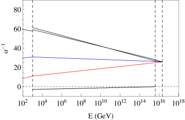
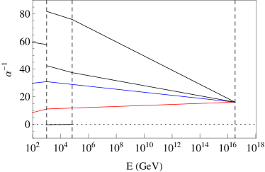
Figure 6: Gauge coupling unification in models with an $U(1)_{R}\times U(1)_{B-L}$ intermediate scale, for $m_{R}=10^{3}$ GeV. Left: $(\Delta b^{LR}_{3},\Delta b^{LR}_{L},\Delta b^{LR}_{R},\Delta b^{LR}_{B-L},\Delta b^{B-L}_{3},\Delta b_{L}^{B-L},\Delta\gamma_{RR},\Delta\gamma_{XR},\Delta\gamma_{XX})=(0,1,3,3,0,0,1/2,-\sqrt{3/8},3/4)$. Right: ($2,2,4,8,2,2,1/2,-\sqrt{3/8},11/4$). The line, which appears close to zero in the $U(1)_{R}\times U(1)_{B-L}$ regime is the running of the off-diagonal element of the matrix $A^{-1}$, i.e. measures the size of the $U(1)$-mixing in the model.

For models in this class, the sliding condition requires that the unification scale is independent of $m_{B-L}$ and this happens when

$$0= \begin{pmatrix}\Delta b_{3}^{B-L}-\Delta b_{2}^{B-L},&p_{Y}^{T}\cdot\Delta\gamma\cdot p_{Y}-\Delta b_{2}^{B-L}\end{pmatrix}.\begin{pmatrix}\begin{array}[]{rr}0&1\\ -1&0\end{array}\end{pmatrix}.\begin{pmatrix}\Delta b_{3}^{LR}-\Delta b_{2}^{LR}\\ \frac{3}{5}\Delta b_{R}^{LR}+\frac{2}{5}\Delta b_{B-L}^{LR}-\Delta b_{2}^{LR}-\frac{18}{5}\end{pmatrix}.$$ (25)

Similarly to PS models, in this class of models the higher intermediate scale ($m_{R}$) depends, in general, on the lower one ($m_{B-L}$). However, there is also here a special condition which makes both $m_{R}$ and $m_{G}$ simultaneously independent of $m_{B-L}$, which is

$$\Delta b_{3}^{LR}=\Delta b_{2}^{LR}=p_{Y}^{T}\cdot\Delta\gamma\cdot p_{Y}.$$ (26)

Models of this kind are, for example, those with $\Delta b_{3}=0$ and $m_{R}$ large, namely $m_{R}\geq 10^{13}$ GeV. One case is given by the model in DeRomeri:2011ie , where $m_{R}\simeq 4\times 10^{15}$ GeV.

III Invariants

III.1 Leading-Log RGE Invariants

In this section we briefly recall the basic definitions DeRomeri:2011ie for the calculation of the “invariants” Buckley:2006nv ; Hirsch:2008gh ; Esteves:2010ff . In mSugra there are four continuous and one discrete parameter: The common gaugino mass $M_{1/2}$, the common scalar mass $m_{0}$, the trilinear coupling $A_{0}$ and the choice of the sign of the $\mu$-parameter, sgn($\mu$). In addition, the ratio of vacuum expectation values of $H_{d}$ and $H_{u}$, $\tan\beta=\frac{v_{u}}{v_{d}}$ is a free parameter. The latter is the only one defined at the weak scale, while all the others are assigned a value at the GUT scale.

Gaugino masses scale as gauge couplings do and so the requirement of GCU fixes the gaugino masses at the low scale

$$M_{i}(m_{SUSY})=\frac{\alpha_{i}(m_{SUSY})}{\alpha_{G}}M_{1/2}.$$ (27)

Neglecting the Yukawa and soft trilinear couplings for the soft mass parameters of the first two generations of sfermions one can write

$$m_{\tilde{f}}^{2}-m_{0}^{2} =\frac{M_{1/2}^{2}}{2\pi\alpha_{G}^{2}}\sum_{R_{j}}\sum_{i=1}^{N}c_{i}^{f,R_{j}}\alpha_{i-}^{R_{j}}\alpha_{i+}^{R_{j}}\left(\alpha_{i-}^{R_{j}}+\alpha_{i+}^{R_{j}}\right)\log\frac{m_{+}^{R_{j}}}{m_{-}^{R_{j}}}\,.$$ (28)

Here, the sum over “$R_{j}$” runs over the different regimes in the models under consideration, while the sum over $i$ runs over all gauge groups in a given regime. $m_{+}^{R_{j}}$ and $m_{-}^{R_{j}}$ are the upper and lower boundaries of the $R_{j}$ regime and $\alpha_{i+}^{R_{j}}$, $\alpha_{i-}^{R_{j}}$ are the values of the gauge coupling of group $i$, $\alpha_{i}$, at these scales. As for the coefficients $c_{i}$, they can be calculated from the quadratic Casimir of representations of each field under each gauge group $i$ and are given for example in DeRomeri:2011ie . In the presence of multiple U(1) gauge groups the RGEs are different (see for instance Fonseca:2011vn and references contained therein) and this leads to a generalization of equation (28) for the U(1) mixing phase DeRomeri:2011ie . Here we just quote the end result (with a minor correction to the one shown in this last reference) ignoring the non-U(1) groups:

$$\tilde{m}_{f-}^{2}-\tilde{m}_{f+}^{2} =\frac{M_{1/2}^{2}}{\pi\alpha_{G}^{2}}Q_{f}^{T}A_{-}\left(A_{-}+A_{+}\right)A_{+}Q_{f}\log\frac{m_{+}}{m_{-}},$$ (29)

where $m_{+}$ and $m_{-}$ are the boundary scales of the U(1) mixing regime and $A_{+}$, $A_{-}$ are the $A$ matrix defined in the previous section (which generalizes $\alpha$) evaluated in these two limits. Likewise, $\tilde{m}_{f+}^{2}$ and $\tilde{m}_{f-}^{2}$ are the values of the soft mass parameter of the sfermion $\tilde{f}$ at these two energy scales. The equation above is a good approximation to the result obtained by integration of the following 1-loop RGE for the soft masses which assumes unification of gaugino masses and gauge coupling constants:

$$\frac{d}{dt}\tilde{m}_{f}^{2} =-\frac{4M_{1/2}^{2}}{\alpha_{G}^{2}}Q_{f}^{T}A^{3}Q_{f}.$$ (30)

Note that in the limit where the U(1) mixing phase extends all the way up to $m_{G}$, the $A$ matrix measured at different energy scales will always commute and therefore equation (29) presented here matches the one in DeRomeri:2011ie and in fact both are exact integrations of (30). However, if this is not the case, it is expected that there will be a small discrepancy between the two approximations, which nevertheless is numerically small and therefore negligible.

From the five soft sfermion mass parameters of the MSSM and one of the gaugino masses it is possible to form four different combinations that, at 1-loop level in the leading-log approximation, do not depend on the values of $m_{0}$ and $M_{1/2}$ and are therefore called invariants:

$$LE =({m_{\widetilde{L}}^{2}-m_{\widetilde{E}}^{2}})/{M_{1}^{2}},$$ (31)

$$QE =({m_{\widetilde{Q}}^{2}-m_{\widetilde{E}}^{2}})/{M_{1}^{2}},$$

$$DL =({m_{\widetilde{D}}^{2}-m_{\widetilde{L}}^{2}})/{M_{1}^{2}},$$

$$QU =({m_{\widetilde{Q}}^{2}-m_{\widetilde{U}}^{2}})/{M_{1}^{2}}.$$

While being pure numbers in the MSSM, invariants depend on the particle content and gauge group in the intermediate stages, as shown by eq. (28).

We will not discuss errors in the calculation of the invariants in detail, we refer the interested reader to DeRomeri:2011ie and for classical $SU(5)$ based SUSY seesaw models to Hirsch:2008gh ; Esteves:2010ff .

We close this subsection by discussing that not all model variants which we presented in section II will be testable by measurements involving invariants at the LHC. According to Baer:2012vr the LHC at $\sqrt{s}=14$ TeV will be able to explore SUSY masses up to $m_{\tilde{g}}\sim 3.2$ TeV ($3.6$ TeV) for $m_{\tilde{q}}\simeq m_{\tilde{g}}$ and of $m_{\tilde{g}}\sim 1.8$ TeV ($2.3$ TeV) for $m_{\tilde{q}}\gg m_{\tilde{g}}$ with 300 fb^-1 (3000 fb^-1). The LEP limit on the chargino, $m_{\chi}>105$ GeV Beringer:1900zz , translates into a lower bound for $M_{1/2}$, with the value depending on the $\Delta b$. For the class-I models with $\Delta b=5$ this leads to $M_{1/2}\raise 1.29167pt\hbox{$\;>$\kern-7.5pt\raise-4.73611pt\hbox{$\sim\;$}}1.06$ TeV. One can assume conservatively $m_{0}=0$ GeV and calculate from this lower bound on $M_{1/2}$ a lower limit on the expected squark masses in the different variants. All variants with squark masses above the expected reach of the LHC-14 will then not be testable via measurements of the invariants. This discards all models with $\Delta b=5$ as untestable unfortunately.

For completeness we mention that if we take the present LHC limit on the gluino, $m_{\tilde{g}}\raise 1.29167pt\hbox{$\;>$\kern-7.5pt\raise-4.73611pt\hbox{$\sim\;$}}1.1$ TeV ATLAS-CONF-2012-109 , this will translate into a lower limit $M_{1/2}\raise 1.29167pt\hbox{$\;>$\kern-7.5pt\raise-4.73611pt\hbox{$\sim\;$}}4.31$ TeV for $\Delta b=5$. We have also checked that models with $\Delta b=4$, can still have squarks with masses testable at LHC, even for the more recent LHC bound on the gluino mass.

III.2 Classification for invariants

The invariants defined in eq. (31) are pure numbers in mSugra and receive corrections which can, in principle, either be positive or negative once new superfields (and/or gauge groups) are added to the MSSM. If we simply consider whether invariants are larger or smaller than their respective values in mSugra, with four invariants there are in principle $2^{4}=16$ possibilities. We arbitrarily assign each of them a number as listed in table 3.

Set #	1	2	3	4	5	6	7	8	9	10	11	12	13	14	15	16
$\Delta LE$	+	+	+	+	+	+	+	+	$-$	$-$	$-$	$-$	$-$	$-$	$-$	$-$
$\Delta QE$	+	+	+	$-$	+	$-$	$-$	$-$	+	+	+	$-$	+	$-$	$-$	$-$
$\Delta DL$	+	+	$-$	+	$-$	+	$-$	$-$	+	+	$-$	+	$-$	+	$-$	$-$
$\Delta QU$	+	$-$	+	+	$-$	$-$	+	$-$	+	$-$	+	+	$-$	$-$	+	$-$
Class-I?	✓	✓								✓				✓
Class-II?	✓	✓	✓			✓	✓	✓		✓				✓		✓
Class-III?	✓	✓								✓				✓

Table 3: The 16 different combinations of signs for 4 invariants. We assign a “$+$” if the corresponding invariant at $m_{SUSY}$ is larger than its value in mSugra and “$-$” otherwise. As discussed in the text, only 9 of the 16 different sign combinations can be realized in the models we consider. Moreover, for class-I only the sets 1,2, 10 and 14 can be realized, see discussion. For class-III we also have found only sets 1,2, 10 and 14, but here our search was not exhaustive.

However, it is easy to demonstrate that not all of the 16 sets can be realized in the three classes of models we consider. This can be understood as follows. If all sfermions have a common $m_{0}$ at the GUT scale, then one can show that

$$m_{\widetilde{E}}^{2}-m_{\widetilde{L}}^{2}+m_{\widetilde{D}}^{2}-2m_{\widetilde{U}}^{2}+m_{\widetilde{Q}}^{2}=0$$ (32)

holds independent of the energy scale, at which soft masses are evaluated. This relation is general, regardless of the combination of intermediate scales that we may consider and for all gauge groups we consider. It is a straightforward consequence of the charge assignments of the standard model fermions and can be easily checked by calculating the Dynkin coefficients of the E,L,D,U and Q representation in the different regimes. In terms of the invariants, this relation becomes:

$$QE=DL+2QU,$$ (33)

i.e. only three of the four invariants are independent. From eq. (33) it is clear that if $\Delta DL$ and $\Delta QU$ are both positive (negative), then $\Delta QE$ must be also positive (negative). This immediately excludes the sets 4, 5, 12 and 13.

Within the MSSM group eq. (32) allows one relation among the invariants. However, one can calculate the relations among the Dynkin indices of the MSSM sfermions within the extended gauge groups we are considering and in these there is one additional relation:

$$QU=LE.$$ (34)

Since eq. (34) is valid only in the regime(s) with extended gauge group(s), it is not exact, once the running within the MSSM regime is included. However, taking into account the running within the MSSM group one can write:

$$QU=LE+f(m_{R}),$$ (35)

with

$$f\left(m_{R}\right)=\frac{2}{33}\left\{\left[\frac{33}{10\pi}\alpha_{1}^{MSSM}\log\left(\frac{m_{R}}{m_{SUSY}}\right)-1\right]^{-2}-1\right\}$$ (36)

Here, $\alpha_{1}^{\rm MSSM}$ is the value of $\alpha_{1}$ at $m_{SUSY}$. It is easy to see that $f(m_{R})$ is always small ($<0.3$) and positive and, vanishes if $m_{R}$ approaches $m_{SUSY}$. Note, that here $m_{R}$ stands for the scale where the MSSM group is extended, in the class-III models it is therefore $m_{B-L}$.

Eq. (35) allows to eliminate three more cases from table 3. Since $f(m_{R})$ is positive, $\Delta QU\leq\Delta LE$ always, so, it is not possible to have $\Delta LE=-$ and $\Delta QU=+$. This excludes three additional sets from table 3: 9, 11 and 15, leaving a total of 9 possible sets.

Finally, in class-I models it is possible to eliminate four more sets, namely all of those with $\Delta DL<0$. It is easy to see, with the help of eq.(28) that this is the case. It follows from the fact that in the LR case, the $c^{L}_{i}$ are non-zero for $U(1)_{B-L}$ and $SU(2)_{L}$ with the values $3/4$ and $3/2$, respectively. Since also the sum is smaller than the $c^{D}_{3}$ (and $\alpha_{3}$ is larger than the other couplings, $D$ must run faster than $L$ in the LR-regime.

By the above reasoning set 6 seems to be, in principle, possible in class-I, but is not realized in our complete scan. We found a few examples in class-II, see below. Due to the (approximate) relation QU=LE it seems a particularly fine-tuned situation. We also note in passing, that in the high-scale seesaw models of type-II Hirsch:2008gh and seesaw type-III Esteves:2010ff with running only within the MSSM group, all invariants run always towards larger values, i.e. only set 1 is realized in this case.

The above discussion serves only as a general classification of the types of sets of invariants that can be realized in the different model classes. The numerical values of the invariants, however, depend on both, the variant of the model class and the scale of the symmetry breaking. We will discuss one example for each possible set next.

III.3 Invariants in model class-I

Fig. (7) shows examples of the $m_{R}$ dependence of the invariants corresponding to the four cases: sets 1, 2, 10 and 14 of table 3. Note that we have scaled down the invariants $QE$ and $DL$ for practical reasons. Note also the different scales in the different plots.

Set 1	Set 2
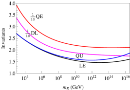
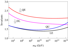
Set 10	Set 14

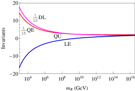
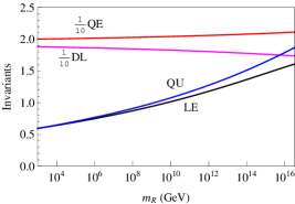
Figure 7: $m_{R}$ dependence of the invariants in model class-I. The examples of $\Delta b^{LR}_{i}=(\Delta b^{LR}_{3},b^{LR}_{L},\Delta b^{LR}_{R},\Delta b^{LR}_{BL})$ for these sets are as follows. Set 1: ($2,2,9,1/2$), Set 2: ($1,1,7,1$), Set 10: ($4,4,3,29/2$), Set 14: ($0,0,2,6$). For a discussion see text.

In all cases QU $\simeq$ LE, if the LR scale extends to very low energies. As explained above, this is a general feature of the extended gauge groups we consider and thus, measuring a non-zero QU-LE allows in our setups, in principle, to derive a lower limit on the scale at which the extended gauge group is broken.

Sets 1 and 2 show a quite similar overall behavior in these examples. Set 1, however, can also be found in variants of class-I with larger $\beta$ coefficients, i.e. larger quantitative changes with respect to the mSugra values. It is possible to find variants within class-I which fall into set 2, but again due to the required similarity of QU and LE, this set can be realized only if both QU and LE are numerically very close to their mSugra values. Set 14 in class-I, finally, is possible only with QE and DL close to their mSugra values, as can be understood from eq. (33).

In general, for variants with large $\Delta b^{LR}_{3}$ changes in the invariants can be huge, see for example the plot shown for set 10. The large change is mainly due to the rapid running of the gaugino masses in these variants, but also the sfermion spectrum is very “deformed” with respect to mSugra expectations. For example, a negative LE means of course that left sleptons are lighter than right sleptons, a feature that can never be found in the “pure” mSugra model. Recall that for solutions with $\Delta b^{LR}_{3}=5$, the value of the squark masses lies beyond the reach of the LHC.

III.4 Model class-II

Fig. (8) shows examples of the invariants for class-II models for those cases of sets, which can not be covered in class-I. Again, QU and DL are scaled and different plots show differently scaled axes.

Set 3	Set 6

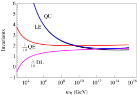
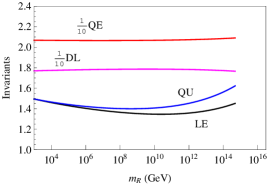
Set 7

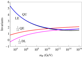
Set 8	Set 16

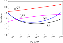
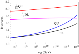
Figure 8: The $m_{R}$ dependence of the invariants in model class-II. The examples shown correspond to the choices of $\Delta b=(\Delta b^{LR}_{3},\Delta b^{LR}_{L},\Delta b^{LR}_{R},\Delta b^{LR}_{BL},\Delta b^{PS}_{4},\Delta b_{L}^{PS},\Delta b_{R}^{PS})$: Set 3: ($0,1,10,3/2,14,9,13$), Set 6: ($0,0,1,9/2,63,60,114$), Set 7: ($0,3,12,1.5,6,3,15$), Set 8: ($0,0,9,1.5,11,8,12$), Set 16: ($0,0,7,1.5,11,8,10$).

The example for set 3 shown in fig. (8) is similar to the one of the original prototype model constructed in DeRomeri:2011ie . For set 6 we have found only a few examples, all of them show invariants which hardly change with respect to the mSugra values of the invariants. The example for set 7 shows that also QE can decrease considerably in some variants with respect to its mSugra value. Set 8 is quantitatively similar to set 2 and set 16 quite similar numerically to set 14. To distinguish these, highly accurate SUSY mass measurements would be necessary.

Again we note that larger values of $\Delta b^{LR}$, especially large $\Delta b^{LR}_{3}$, usually lead to numerically larger changes in the invariants, making these models in principle easier to test.

III.5 Model class-III

$\Delta b_{3}=0$	$\Delta b_{3}\neq 0$

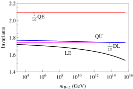
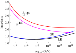
Figure 9: The $m_{B-L}$ dependence of the invariants in Model III. To the left the example chooses: $(\Delta b^{LR}_{3},\Delta b^{LR}_{L},\Delta b^{LR}_{R},\Delta b^{LR}_{BL},\Delta b^{BL}_{3},\Delta b^{BL}_{L},\Delta\gamma_{RR},\Delta\gamma_{XR},\Delta\gamma_{XX})=(0,1,3,3,0,0,1/2,-\sqrt{3/8},3/4)$. To the right: ($2,2,4,8,2,2,1/2,-\sqrt{3/8},11/4$).

Here, the invariants depend on $m_{B-L}$ with a milder or stronger dependence, depending on the value of $\Delta b_{3}$. For almost all the solutions with $\Delta b_{3}=0$ , the values $QU$, $DL$, $QE$ are constants and only in $LE$ a mild variation with $m_{B-L}$ is found. This fact was already pointed out in DeRomeri:2011ie . However, we have found that class-III models can be made with $\Delta b_{3}>0$ and these, in general, lead to invariants which are qualitatively similar to the case of class-I discussed above. In fig. (9) we show two examples of invariants for class-III, one with $\Delta b_{3}=0$ and one with $\Delta b_{3}=1$.

The solutions with $\Delta b_{3}\neq 0$ fall in two kinds: The minimum value of $m_{R}$ is very large. Then, the invariants have the same behavior than those in which $\Delta b_{3}=0$. The minimum value of $m_{R}$ is low. The invariants are not constants and look similar to the ones in the class-I models. The generally mild dependence on $m_{B-L}$ can be understood, since it enters into the soft masses only through the changes in the abelian gauge couplings. Class-III models are therefore the hardest to “test” using invariants.

III.6 Comparison of model classes

The classification of variants that we have discussed in section III.2 only takes into account what happens when the lowest intermediate scale is very low, ${\cal O}(m_{SUSY})$. When one varies continuously the lowest intermediate scale ($m_{R}$ in the LR and PS-class models or $m_{B-L}$ in the BL-class of models), each variant draws a line in the 4-dimensional space $\left(LE,QU,DL,QE\right)$. The dimensionality of such a plot can be lowered if we use the (approximate) relations between the invariants shown above, namely $QU\approx LE$ and $QE=DL+2QU$. We can then choose two independent ones, for example $LE$ and $QE$, so that the only non-trivial information between the 4 invariants is encoded in a $\left(LE,QE\right)$ plot. In this way, it is possible to simultaneous display the predictions of different variants. This was done in fig. (10), where LR-, PS- and BL-variants are drawn together. The plot is exhaustive in the sense that it includes all LR-variants, as well as all PS- and BL-variants which can have the highest intermediate scale below $10^{6}$ GeV. In all cases, we required that $\alpha^{-1}$ at unification is larger than $\nicefrac{{1}}{{2}}$ when the lowest intermediate scale is equal to $m_{SUSY}$.

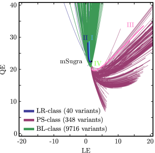
Figure 10: Parametric $\left(LE,QE\right)$ plot for the different variants (see text). The thicker lines labeled with I, II, III and IV indicate the result for the four prototype models presented in DeRomeri:2011ie .

There is a dot in the middle of the figure - the mSugra point - which corresponds to the prediction of mSugra models, in the approximation used. It is expected that every model will draw a line with one end close to this point. This end-point corresponds to the limit where the intermediate scales are close to the GUT scale and therefore the running in the LR, PS and BL phases is small so the invariants should be similar to those in mSugra models. So the general picture is that lines tend to start (when the lowest intermediate scale is of the order of $10^{3}$ GeV) outside or at the periphery of the plot, away from the mSugra point and, as the intermediate scales increase, they converge towards the region of the mSugra point, in the middle of the plot. In fact, note that all the blue lines of LR-class models do touch this point, because we can slide the LR scale all the way to $m_{G}$. But in PS- and BL- models there are two intermediate scales and often the lowest one cannot be increased all the way up to $m_{G}$, either because that would make the highest intermediate scale bigger than $m_{G}$ or because it would invert the natural ordering of the two intermediate scales.

It is interesting to note that the BL-class with low $m_{R}$ can produce the same imprint in the sparticle masses as LR-models. This is to be expected because with $m_{R}$ close to $m_{B-L}$ the running in the U(1)-mixing phase is small, leading to predictions similar to LR-models. The equivalent limit for PS-class models is reached for very high $m_{PS}$, close to the GUT scale (see below). On the other hand, from fig. (10) we can see that a low $m_{PS}$ actually leads to a very different signal on the soft sparticle masses. For example, a measurement of $LE\approx 10$ and $QE\approx 15$, together with compatible values for the other two invariants ($QU\approx 10$ and $DL\approx-5$) would immediately exclude all classes of models except PS-models, and in addition it would strongly suggest low PS and LR scales.

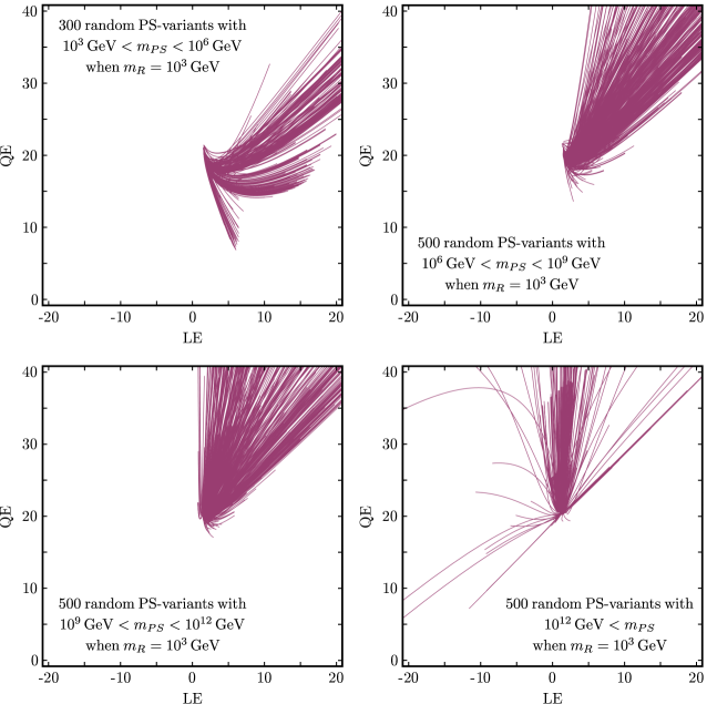
Figure 11: Parametric $\left(LE,QE\right)$ plots for different PS-variants showing the effect of the PS scale.

Fig. (11) illustrates the general behavior of PS-models as we increase the separation between the $m_{LR}$ and $m_{PS}$ scales. The red region in the $\left(LE,QE\right)$ plot tends to rotate anti-clockwise until it reaches, for very high $m_{PS}$, the same region of points which is predicted by LR-models. Curiously, we also see in fig. (11) that some of these models actually predict different invariant values from the ones of LR models. What happens in these cases is that since the PS phase is very short, it is possible to have many active fields in it which decouple at lower energies. So even though the running is short, the values of the different gauge couplings actually get very large corrections in this regime and these are uncommon in other settings. For example, it is possible in this special subclass of PS-models for $\alpha_{R}$ to get bigger than $\alpha_{3}$/$\alpha_{4}$ before unifying!

One can see from fig. (11) that many, although not all PS-models can lead to large values of $LE$. This can happen for both low and high values of $m_{PS}$ and is a rather particular feature of the class-II, which can not be found in the other classes.

IV Summary and conclusions

We have discussed $SO(10)$ based supersymmetric models with extended gauge group near the electro-weak scale, consistent with gauge coupling unification thanks to a “sliding scale” mechanism. We have discussed three different setups, which we call classes of models. The first and simplest chain we use breaks $SO(10)$ through a left-right symmetric stage to the SM group, class-II uses an additional intermediate Pati-Salam stage, while in class-III we discuss models which break the LR-symmetric group first into a $U(1)_{R}\times U(1)_{B-L}$ group before reaching the SM group. We have shown that in each case many different variants and many configurations (or “proto-models”) for each variant can be constructed.

We have discussed that one can not only construct sliding models in which an inverse or linear seesaw is consistent with GCU, as done in earlier work Malinsky:2005bi ; Dev:2009aw ; DeRomeri:2011ie , but also all other known types of seesaws can, in principle, be found. We found example configurations for seesaw type-I, type-II and type-III and even inverse type-III (for which one example limited to class-II was previously discussed in DeRomeri:2011ie ).

Due to the sliding scale property the different configurations predict potentially rich phenomenology at the LHC, although by the same reasoning the discovery of any of the additional particles the models predict is of course not guaranteed. However, even if all the new particles - including the gauge bosons of the extended gauge group - lie outside of the reach of the LHC, indirect tests of the models are possible from measurements of SUSY particle masses. We have discussed certain combinations of soft parameters, called “invariants”, and shown that the invariants themselves can be classified into a few sets. Just determining to which set the experimental data belongs would allow to distinguish, at least in some cases, class-I from class-II models and also in all but one case our classes of models are different from the ordinary high-scale seesaw (type-II and type-III) models. Depending on the accuracy with which supersymmetric masses can be measured in the future, the invariants could be used to gain indirect information not only on the class of model and its variant realized in nature, but also give hints on the scale of beyond-MSSM physics, i.e. the energy scale at which the extended gauge group is broken.

We add a few words of caution. First of all, our analysis is done completely at the 1-loop level. It is known from numerical calculations for seesaw type-II Hirsch:2008gh and seesaw type-III Esteves:2010ff that the invariants receive numerically important shifts at 2-loop level. In addition, there are also uncertainties in the calculation from GUT-scale thresholds and from uncertainties in the input parameters. For the latter the most important is most likely the error on $\alpha_{S}$ DeRomeri:2011ie . With the huge number of models we have considered, taking into account all of these effects is impractical and, thus, our numerical results should be taken as approximate. However, should any signs of supersymmetry be found in the future, improvements in the calculations along these lines could be easily made, should it become necessary. More important for the calculation of the invariants is, of course, the assumption that SUSY breaking indeed is mSugra-like. Tests of the validity of this assumption can be made also only indirectly. Many of the spectra we find, especially in the class-II models, are actually quite different from standard mSugra expectations and thus a pure MSSM-mSugra would give a bad fit to experimental data, if one of these models is realized in nature. However, all of our variants still fulfill (by construction) a certain sum rule, see the discussion in section III.2.

Of course, so far no signs of supersymmetry have been seen at the LHC, but with the planned increase of $\sqrt{s}$ for the next run of the accelerator there is still quite a lot of parameter space to be explored. We note in this respect that we are not overly concerned about the Higgs mass, $m_{h}\sim(125-126)$ GeV, if the new resonance found by the ATLAS ATLAS:2012gk and CMS CMS:2012gu collaborations turns out to be indeed the lightest Higgs boson. While for a pure MSSM with mSugra boundary conditions it is well-known Arbey:2011ab ; Baer:2011ab ; Buchmueller:2011ab ; Ellis:2012aa that such a hefty Higgs requires multi-TeV scalars, all our models have an extended gauge symmetry. Thus, there are new D-terms contributing to the Higgs mass Haber:1986gz ; Drees:1987tp , alleviating the need for large soft SUSY breaking terms, as has been explicitly shown in Hirsch:2012kv ; Hirsch:2011hg for one particular realization of a class-III model Malinsky:2005bi ; DeRomeri:2011ie .

Finally, many of the configuration (or proto-models) which we have discussed contain exotic superfields, which might show up in the LHC. It might therefore be interesting to do a more detailed study of the phenomenology of at least some particular of the models we have constructed.

Appendix A Lists of superfields

We have considered $SO(10)$ based models which may contain any irreducible representation up to dimension 126 ($\boldsymbol{1}$, $\boldsymbol{10}$, $\boldsymbol{16}$, $\overline{\boldsymbol{16}}$, $\boldsymbol{45}$, $\boldsymbol{54}$, $\boldsymbol{120}$, $\boldsymbol{126}$, $\overline{\mathbf{126}}$). Once the gauge group breaks down to $SU(4)\times SU(2)_{L}\times SU(2)_{R}$ or $SU(3)_{C}\times SU(2)_{L}\times SU(2)_{R}\times U(1)_{B-L}$ these $SO(10)$ fields divide into a multitude of different irreducible representation of these groups. In addition, if $SU(2)_{R}$ is broken down further to $U(1)_{R}$ the following branching rules apply: $\boldsymbol{3}\rightarrow-1,0,+1$; $\boldsymbol{2}\rightarrow\pm\frac{1}{2}$; $\boldsymbol{1}\rightarrow 0$. The standard model’s hypercharge, in the canonical normalization, is then equal to the combination $\sqrt{\frac{3}{5}}\left[U(1)_{R}\textrm{ hypercharge}\right]+\sqrt{\frac{2}{5}}\left[U(1)_{B-L}\textrm{ hypercharge}\right]$. In tables 4, 5 and 6 we present the list of relevant fields respecting the conditions above. In these tables we used an ordered naming of the fields. Sometimes it is also useful, like in table 1, to indicate explicitly the quantum numbers under the various groups.

$\Phi_{1}$ $\Phi_{2}$ $\Phi_{3}$ $\Phi_{4}$ $\Phi_{5}$ $\Phi_{6}$ $\Phi_{7}$ $\Phi_{8}$ $\Phi_{9}$ $\Phi_{10}$ $\Phi_{11}$ $\Phi_{12}$ $\Phi_{13}$ $\Phi_{14}$ $\chi$ $\chi^{c}$ $\Omega$ $\Omega^{c}$ $\Phi$ $\delta_{d}$ $\delta_{u}$ $SU(3)_{C}$ 1 1 1 1 1 1 8 1 3 3 6 6 3 3 $SU(2)_{L}$ 1 2 1 3 1 2 1 1 1 1 1 1 2 1 $SU(2)_{R}$ 1 1 2 1 3 2 1 1 1 1 1 1 1 2 $U(1)_{B-L}$ 0 +1 -1 0 0 0 0 +2 $-\frac{2}{3}$ $+\frac{4}{3}$ $+\frac{2}{3}$ $-\frac{4}{3}$ $+\frac{1}{3}$ $+\frac{1}{3}$ PS Origin $\Psi_{1}$ $\Psi_{10}$ $\overline{\Psi}_{12}$ $\Psi_{13}$ $\Psi_{3}$ $\Psi_{4}$ $\Psi_{2}$ $\Psi_{7}$ $\Psi_{10}$ $\Psi_{11}$ $\overline{\Psi}_{9}$ $\Psi_{8}$ $\Psi_{9}$ $\Psi_{10}$ $\Psi_{9}$ $\Psi_{11}$ $\Psi_{12}$ $\Psi_{13}$

$\Phi_{15}$ $\Phi_{16}$ $\Phi_{17}$ $\Phi_{18}$ $\Phi_{19}$ $\Phi_{20}$ $\Phi_{21}$ $\Phi_{22}$ $\Phi_{23}$ $\Phi_{24}$ $\Delta$ $\Delta^{c}$ $SU(3)_{C}$ 8 1 1 3 3 3 6 6 1 3 $SU(2)_{L}$ 2 3 1 2 3 1 3 1 3 2 $SU(2)_{R}$ 2 1 3 2 1 3 1 3 3 2 $U(1)_{B-L}$ 0 -2 -2 $+\frac{4}{3}$ $-\frac{2}{3}$ $-\frac{2}{3}$ $+\frac{2}{3}$ $+\frac{2}{3}$ 0 $-\frac{2}{3}$ PS Origin $\Psi_{7}$ $\Psi_{16}$ $\Psi_{17}$ $\Psi_{7}$ $\Psi_{14}$ $\Psi_{16}$ $\Psi_{15}$ $\Psi_{17}$ $\Psi_{16}$ $\Psi_{17}$ $\Psi_{5}$ $\Psi_{6}$

Table 4: Naming conventions and transformation properties of fields in the left-right symmetric regime (not considering conjugates). The charges under the $U(1)_{B-L}$ group shown here were multiplied by a factor $\sqrt{\frac{8}{3}}$.

	$\Psi_{1}$	$\Psi_{2}$	$\Psi_{3}$	$\Psi_{4}$	$\Psi_{5}$	$\Psi_{6}$	$\Psi_{7}$	$\Psi_{8}$	$\Psi_{9}$	$\Psi_{10}$	$\Psi_{11}$	$\Psi_{12}$	$\Psi_{13}$	$\Psi_{14}$	$\Psi_{15}$	$\Psi_{16}$	$\Psi_{17}$
$SU(4)$	1	1	1	1	1	6	15	6	10	15	20’	4	4	6	6	10	10
$SU(2)_{L}$	1	2	3	1	3	2	2	1	1	1	1	2	1	3	1	3	1
$SU(2)_{R}$	1	2	1	3	3	2	2	1	1	1	1	1	2	1	3	1	3
$SO(10)$ Origin	1 54	10 120	45	45	54	45 54	120 126	10 126	120	45	54	16	$\overline{\mathbf{16}}$	120	120	126	$\overline{\mathbf{126}}$

Table 5: Naming conventions and transformation properties of fields in the Pati-Salam regime (not considering conjugates)

$\Phi_{1}^{{}^{\prime}}$ $\Phi_{2}^{{}^{\prime}}$ $\Phi_{3}^{{}^{\prime}}$ $\Phi_{4}^{{}^{\prime}}$ $\Phi_{5}^{{}^{\prime}}$ $\Phi_{6}^{{}^{\prime}}$ $\Phi_{7}^{{}^{\prime}}$ $\Phi_{8}^{{}^{\prime}}$ $\Phi_{9}^{{}^{\prime}}$ $\Phi_{10}^{{}^{\prime}}$ $\Phi_{11}^{{}^{\prime}}$ $\Phi_{12}^{{}^{\prime}}$ $\Phi_{13}^{{}^{\prime}}$ $\Phi_{14}^{{}^{\prime}}$ $\Phi_{15}^{{}^{\prime}}$ $\Phi_{16}^{{}^{\prime}}$ $SU(3)_{C}$ 1 1 1 1 1 1 1 8 1 3 3 6 6 3 3 3 $SU(2)_{L}$ 1 2 1 1 3 1 2 1 1 1 1 1 1 2 1 1 $U(1)_{R}$ 0 0 $-\frac{1}{2}$ $+\frac{1}{2}$ 0 +1 $+\frac{1}{2}$ 0 0 0 0 0 0 0 $-\frac{1}{2}$ $+\frac{1}{2}$ $U(1)_{B-L}$ 0 +1 -1 -1 0 0 0 0 +2 $-\frac{2}{3}$ $+\frac{4}{3}$ $+\frac{2}{3}$ $-\frac{4}{3}$ $+\frac{1}{3}$ $+\frac{1}{3}$ $+\frac{1}{3}$ LR Origin $\Phi_{1}$ $\Phi_{5}$ $\Phi_{2}$ $\Phi_{3}$ $\Phi_{3}$ $\Phi_{4}$ $\Phi_{23}$ $\Phi_{5}$ $\Phi_{6}$ $\Phi_{7}$ $\Phi_{8}$ $\bar{\Phi}_{17}$ $\Phi_{9}$ $\Phi_{20}$ $\Phi_{10}$ $\Phi_{11}$ $\Phi_{22}$ $\Phi_{12}$ $\Phi_{13}$ $\Phi_{14}$ $\Phi_{14}$

$\Phi_{17}^{{}^{\prime}}$ $\Phi_{18}^{{}^{\prime}}$ $\Phi_{19}^{{}^{\prime}}$ $\Phi_{20}^{{}^{\prime}}$ $\Phi_{21}^{{}^{\prime}}$ $\Phi_{22}^{{}^{\prime}}$ $\Phi_{23}^{{}^{\prime}}$ $\Phi_{24}^{{}^{\prime}}$ $\Phi_{25}^{{}^{\prime}}$ $\Phi_{26}^{{}^{\prime}}$ $\Phi_{27}^{{}^{\prime}}$ $\Phi_{28}^{{}^{\prime}}$ $\Phi_{29}^{{}^{\prime}}$ $\Phi_{30}^{{}^{\prime}}$ $\Phi_{31}^{{}^{\prime}}$ $SU(3)_{C}$ 8 1 1 1 3 3 3 3 3 6 6 6 1 3 3 $SU(2)_{L}$ 2 3 1 1 2 2 3 1 1 3 1 1 3 2 2 $U(1)_{R}$ $+\frac{1}{2}$ 0 -1 +1 $-\frac{1}{2}$ $+\frac{1}{2}$ 0 -1 +1 0 -1 +1 +1 $-\frac{1}{2}$ $+\frac{1}{2}$ $U(1)_{B-L}$ 0 -2 -2 -2 $+\frac{4}{3}$ $+\frac{4}{3}$ $-\frac{2}{3}$ $-\frac{2}{3}$ $-\frac{2}{3}$ $+\frac{2}{3}$ $+\frac{2}{3}$ $+\frac{2}{3}$ 0 $-\frac{2}{3}$ $-\frac{2}{3}$ LR Origin $\Phi_{15}$ $\Phi_{16}$ $\Phi_{17}$ $\Phi_{17}$ $\Phi_{18}$ $\Phi_{18}$ $\Phi_{19}$ $\Phi_{20}$ $\Phi_{20}$ $\Phi_{21}$ $\Phi_{22}$ $\Phi_{22}$ $\Phi_{23}$ $\Phi_{24}$ $\Phi_{24}$

Table 6: Naming conventions and transformation properties of fields in the U(1) mixing regime (not considering conjugates). The charges under the $U(1)_{B-L}$ group shown here were multiplied by a factor $\sqrt{\frac{8}{3}}$.

In order for a group $G$ to break into a subgroup $H\subset G$, there must be a field transforming non-trivially under $G$ which contains a singlet of $H$ that acquires vacuum expectation value. From this observation alone we know that certain fields must be present in a fundamental model if we are to achieve a given breaking sequence:

• The breaking $PS\rightarrow LR$ is possible only with the (15,1,1) while $PS\rightarrow 3211$ requires the combination (15,1,1) + (1,1,3). For the direct breaking $PS\rightarrow 321$ there are two choices: (4,1,2), (10,1,3) or their conjugates;

• The breaking $LR\rightarrow 3211$ requires the (1,1,3,0) representation while the direct route $LR\rightarrow 321$ is possible with the presence of (1,1,2,-1), (1,1,3,-2) or their conjugates;

• The group $3211$ can be broken down to $321$ with the representations $(\boldsymbol{1},\boldsymbol{1},\frac{1}{2},-1)$, $(\boldsymbol{1},\boldsymbol{1},1,-2)$ or their conjugates.

References

- (1) Super-Kamiokande Collaboration, Y. Fukuda et al., Phys.Rev.Lett. 81, 1562 (1998), arXiv:hep-ex/9807003.
- (2) SNO Collaboration, Q. Ahmad et al., Phys.Rev.Lett. 89, 011301 (2002), arXiv:nucl-ex/0204008.
- (3) KamLAND Collaboration, K. Eguchi et al., Phys.Rev.Lett. 90, 021802 (2003), arXiv:hep-ex/0212021.
- (4) D. Forero, M. Tortola, and J.W.F. Valle, Phys.Rev. D86, 073012 (2012), arXiv:1205.4018.
- (5) P. Minkowski, Phys.Lett. B67, 421 (1977).
- (6) T. Yanagida, KEK lectures, ed. O. Sawada and A. Sugamoto, Tsukuba, Japan (1979).
- (7) M. Gell-Mann, P. Ramond, and R. Slansky, Conf.Proc. C790927, 315 (1979).
- (8) R. N. Mohapatra and G. Senjanovic, Phys.Rev.Lett. 44, 912 (1980).
- (9) H. Fritzsch and P. Minkowski, Annals Phys. 93, 193 (1975).
- (10) R. N. Mohapatra, Contemporary Physics (Springer, Berlin, Germany) (1986).
- (11) M. Cvetic and J. C. Pati, Phys.Lett. B135, 57 (1984).
- (12) R. Kuchimanchi and R. Mohapatra, Phys.Rev. D48, 4352 (1993), arXiv:hep-ph/9306290.
- (13) C. S. Aulakh, K. Benakli, and G. Senjanovic, Phys.Rev.Lett. 79, 2188 (1997), arXiv:hep-ph/9703434.
- (14) C. S. Aulakh, A. Melfo, A. Rasin, and G. Senjanovic, Phys.Rev. D58, 115007 (1998), arXiv:hep-ph/9712551.
- (15) S. K. Majee, M. K. Parida, A. Raychaudhuri, and U. Sarkar, Phys.Rev. D75, 075003 (2007), arXiv:hep-ph/0701109.
- (16) V. De Romeri, M. Hirsch, and M. Malinsky, Phys.Rev. D84, 053012 (2011), arXiv:1107.3412.
- (17) L. Calibbi, L. Ferretti, A. Romanino, and R. Ziegler, Phys.Lett. B672, 152 (2009), arXiv:0812.0342.
- (18) M. Malinsky, J. Romao, and J.W.F. Valle, Phys.Rev.Lett. 95, 161801 (2005), arXiv:hep-ph/0506296.
- (19) P. B. Dev and R. Mohapatra, Phys.Rev. D81, 013001 (2010), arXiv:0910.3924.
- (20) J. C. Pati and A. Salam, Phys.Rev. D10, 275 (1974).
- (21) M. R. Buckley and H. Murayama, Phys.Rev.Lett. 97, 231801 (2006), arXiv:hep-ph/0606088.
- (22) M. Hirsch, S. Kaneko, and W. Porod, Phys.Rev. D78, 093004 (2008), arXiv:0806.3361.
- (23) J. Esteves, J. Romao, M. Hirsch, F. Staub, and W. Porod, Phys.Rev. D83, 013003 (2011), arXiv:1010.6000.
- (24) Particle Data Group, J. Beringer et al., Phys.Rev. D86, 010001 (2012).
- (25) J. Romao et al., http://porthos.ist.utl.pt/arXiv/AllSO10GUTs.
- (26) R. N. Mohapatra and J. W. F. Valle, Phys. Rev. D34, 1642 (1986).
- (27) E. K. Akhmedov, M. Lindner, E. Schnapka, and J.W.F. Valle, Phys.Lett. B368, 270 (1996), arXiv:hep-ph/9507275.
- (28) E. K. Akhmedov, M. Lindner, E. Schnapka, and J.W.F. Valle, Phys.Rev. D53, 2752 (1996), arXiv:hep-ph/9509255.
- (29) R. Foot, H. Lew, X. He, and G. C. Joshi, Z.Phys. C44, 441 (1989).
- (30) K. Babu, B. Dutta, and R. Mohapatra, Phys.Rev. D60, 095004 (1999), arXiv:hep-ph/9812421.
- (31) S. Davidson, D. C. Bailey, and B. A. Campbell, Z.Phys. C61, 613 (1994), arXiv:hep-ph/9309310.
- (32) A. Kuznetsov, N. Mikheev, and A. Serghienko, (2012), arXiv:1210.3697.
- (33) R. M. Fonseca, M. Malinsky, W. Porod, and F. Staub, Nucl.Phys. B854, 28 (2012), arXiv:1107.2670.
- (34) H. Baer, V. Barger, A. Lessa, and X. Tata, (2012), arXiv:1207.4846.
- (35) ATLAS Collaboration, G. Aad et al., ATLAS-CONF-2012-109 (2012).
- (36) ATLAS Collaboration, G. Aad et al., Phys.Lett. B716, 1 (2012), arXiv:1207.7214.
- (37) CMS Collaboration, S. Chatrchyan et al., Phys.Lett. B716, 30 (2012), arXiv:1207.7235.
- (38) A. Arbey, M. Battaglia, A. Djouadi, F. Mahmoudi, and J. Quevillon, Phys.Lett. B708, 162 (2012), arXiv:1112.3028.
- (39) H. Baer, V. Barger, and A. Mustafayev, Phys.Rev. D85, 075010 (2012), arXiv:1112.3017.
- (40) O. Buchmueller et al., Eur.Phys.J. C72, 2020 (2012), arXiv:1112.3564.
- (41) J. Ellis and K. A. Olive, Eur.Phys.J. C72, 2005 (2012), arXiv:1202.3262.
- (42) M. Hirsch, F. Joaquim, and A. Vicente, JHEP 1211, 105 (2012), arXiv:1207.6635.
- (43) H. E. Haber and M. Sher, Phys.Rev. D35, 2206 (1987).
- (44) M. Drees, Phys.Rev. D35, 2910 (1987).
- (45) M. Hirsch, W. Porod, L. Reichert, and F. Staub, Phys.Rev. D86, 093018 (2012), arXiv:1206.3516.
- (46) M. Hirsch, M. Malinsky, W. Porod, L. Reichert, and F. Staub, JHEP 1202, 084 (2012), arXiv:1110.3037.