A Physical Model for the Revised Blazar Sequence

Abstract

The blazar sequence is reflected in a correlation of the peak luminosity versus peak frequency of the synchrotron component of blazars. This correlation has been considered one of the fundamental pieces of evidence for the existence of a continuous sequence that includes low-power BL Lacertae objects through high-power flat spectrum radio quasars. A correlation between the Compton dominance, the ratio of the Compton to synchrotron luminosities, and the peak synchrotron frequency is another piece of evidence for the existence of the blazar sequence explored by Fossati et al. (1998). Since that time, however, it has essentially been ignored. We explore this correlation with a sample based on the second LAT AGN catalog (2LAC), and show that is is particularly important, since it is independent of redshift. We reproduce the trends in our sample with a simple model that includes synchrotron and Compton cooling in the slow- and fast-cooling regimes, and angle-dependent effects.

I Introduction

Active Galactic Nuclei (AGN) with relativistic jets pointed along our line of sight are known collectively as blazars. This includes those with strong broad emission lines, Flat Spectrum Radio Quasars (FSRQs), and those with weak or absent lines, known as BL Lacertae objects (BL Lacs; marcha96, ). In general, the spectral energy distributions (SEDs) of blazars have two basic components: a low frequency component, peaking in the optical through X-rays, from synchrotron emission, and a high frequency component, peaking in the $\gamma$ rays, probably originating from Compton scattering of some seed photon source, either internal (synchrotron self-Compton or SSC) or external to the jet (external Compton or EC).

Aside from their classifications as FSRQs or BL Lacs from optical spectra, abdo10_sed subdivided them based on their synchrotron peak. They are considered high synchrotron-peaked (HSP) blazars if their synchrotron peak $\nu^{sy}_{pk}>10^{15}\ \mathrm{Hz}$; intermediate synchrotron-peaked (ISP) blazars if $10^{14}\ \mathrm{Hz}<\nu^{sy}_{pk}<10^{15}\ \mathrm{Hz}$; and low synchrotron-peaked (LSP) blazars if $\nu^{sy}_{pk}<10^{14}\ \mathrm{Hz}$. Almost all FSRQs are LSP blazars.

fossati98 combined several blazar surveys and noticed an anti-correlation between the luminosity at the synchrotron peak, $L_{pk}^{sy}$, and the frequency of this peak, $\nu^{sy}_{pk}$. They also noticed anti-correlations between the 5 GHz luminosity $L_{5\ GHz}$ and $\nu^{sy}_{pk}$, the $\gamma$-ray luminosity and $\nu^{sy}_{pk}$, and the $\gamma$-ray dominance (the ratio of the EGRET $\gamma$-ray luminosity to the synchrotron peak luminosity) and $\nu^{sy}_{pk}$. ghisellini98 provided a physical explanation for these correlations (see also boett02_seq, ). If the seed photon source for external Compton scattering is the broad-line region (BLR), and the BLR strength is correlated with the power injected into electrons in the jet, one would expect that more luminous jets have stronger broad emission lines and greater Compton cooling, and thus a lower $\nu^{sy}_{pk}$. As the power injected in electrons is reduced, the broad line luminosity decreases, there are fewer seed photons for Compton scattering, and consequently the peak synchrotron frequency moves to higher frequencies. This is also reflected in the lower luminosity of the Compton-scattered component relative to the synchrotron component as $\nu^{sy}_{pk}$ moves to higher frequencies.

The $L_{pk}^{sy}$–$\nu_{pk}^{sy}$ anti-correlation has been questioned. Using blazars from two large surveys, padovani03 did not find any anti-correlation between $\nu^{sy}_{pk}$ and radio, BLR, or jet power. This work, however, has been criticized for its relatively poor SED characterization (ghisellini08_seq, ). Also, the lack of sources in the upper right region of the $L_{pk}^{sy}$–$\nu_{pk}^{sy}$ plot could be the result of a selection effect (giommi02, ; padovani02, ; giommi05, ; giommi11_selection). Since a large fraction of BL Lac objects have entirely featureless optical spectra, their redshifts, $z$, and hence luminosities, are impossible to determine. These could be extremely bright, distant BL Lacs that would fill in the upper right region. nieppola06 found no correlation between the frequency and luminosity of the synchrotron peaks for objects in the Metsähovi Radio Observatory BL Lacertae sample. chen11 did find an anti-correlation, using sources found in the LAT bright AGN sample (abdo09_lbas, ; abdo10_sed, ). In recent works, an “L”-shape in the $L_{pk}^{sy}$–$\nu_{pk}^{sy}$ plot seems to have emerged, as lower luminosity and low-peaked sources have been detected with more sensitive instruments (meyer11, ; giommi12, ). nieppola06 found more of a “V” shape, although their plot did not include FSRQs; if high luminosity and low-peaked FSRQs were added, it might appear as more of an “L”. With the advent of the Fermi Telescope era, it is now possible to also characterize the Compton peak frequency $\nu_{pk}^{C}$ and luminosity $L_{pk}^{C}$. As we show, the Compton dominance $A_{C}\equiv L_{pk}^{C}/L_{pk}^{sy}$ is an important parameter for charcterizing this sequence.

II The 2LAC Blazar Sequence

The 2LAC (ackermann11_2lac, ) allows for the characterization of the high energy component for a greater number of blazars than previously possible. Here we look at the blazar sequence among the 2LAC clean sample, which includes 885 total sources, with 395 BL Lacs, 310 FSRQs, and 156 sources of unknown type.

abdo10_sed fit the broadband SEDs of the blazars in the 3-month LAT bright AGN sample (LBAS; abdo09_lbas, ) with third degree polynomials to determine the peak synchrotron frequency, $\nu_{pk}^{sy}$. abdo10_sed found empirical relations for finding the peak frequency of the synchrotron component from the slope between the 5 GHz and 5000 Å flux ($\alpha_{ro}$), and between the 5000 Å and 1 keV flux ($\alpha_{ox}$). ackermann11_2lac used these empirical relations and their low energy data to determine $\nu_{pk}^{sy}$ for the 2LAC sample. This was then used to classify the SEDs of the blazars as LSP, ISP, or HSP. abdo10_sed also provided an empirical formula for determining the flux at the synchrotron peak from the the 5 GHz flux density and $\nu_{pk}^{sy}$. We used this relation, along with the $\nu_{pk}^{sy}$ values from the 2LAC (ackermann11_2lac, ) to get the luminosity distance and create a plot of the peak synchrotron luminosity, $L^{sy}_{pk}$ versus $\nu_{pk}^{sy}$. This is plotted in Fig. 1. These are the sources in the 2LAC clean sample with measured redshifts and enough SED measurements to determine $\nu_{pk}^{sy}$, which amounts to 352 sources including 145 BL Lacs, 195 FSRQs, and 12 AGN of unknown optical spectral type (AGUs; i.e., unknown whether they are FSRQs or BL Lacs). Note that $\nu_{pk}^{sy}$ is corrected for redshift, and is in the frame of the source. We include the photometric redshifts which have been determined from rau12 .

For this diagram, we have computed the Spearman ($\rho$) and Kendall ($\tau$) rank correlation coefficients and the probability of no correlation (PNC) calculated from each coefficient. The results can be found in Table 1. The results from $\rho$ and $\tau$ are similar in all cases. The PNC is very small for the BL Lacs and FSRQs separately, and even lower for all the sources combined, where the probability is essentially zero that there is not a correlation. Note however, that, sources with unknown $z$ are not included. This could explain the anti-correlations for the whole sample and for the BL Lacs in general giommi12_selection , since they could fill in the upper right part of this diagram, as mentioned in Section I. However, the objects with unknown $z$ are almost certainly BL Lacs, so it would not explain any possible anti-correlation amoung the FSRQs alone, although no significant one was found.

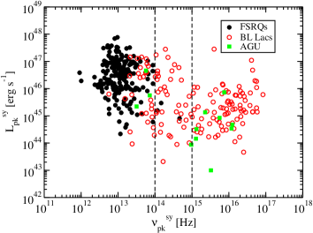
Figure 1: Peak synchrotron luminosity versus peak synchrotron frequency for objects in the 2LAC clean sample. Filled circles represent FSRQs, empty circles represent BL Lacs, and filled squares represent objects which do not have an unambiguous classification. Dashed lines indicate the boundary between HSPs and ISPs and between ISPs and LSPs.

Table 1: Statistics of correlations involving $\nu_{pk}^{sy}$.

Sample	$\rho$	PNC($\rho$)	$\tau$	PNC($\tau$)
$L_{pk}^{sy}$ versus $\nu_{pk}^{sy}$
BL Lacs	-0.19	0.019	-0.12	0.035
FSRQs	-0.12	0.073	-0.088	0.066
All sources with known $z$	-0.54	$4.2\times 10^{-28}$	-0.35	0.00
$L_{5GHz}$ versus $\nu_{pk}^{sy}$
BL Lacs	-0.64	$5.4\times 10^{-18}$	-0.45	0.00
FSRQs	-0.36	$1.82\times 10^{-7}$	-0.25	$1.79\times 10^{-7}$
All sources with known $z$	-0.79	0.00	-0.58	0.00
$A_{C}$ versus $\nu_{pk}^{sy}$
BL Lacs	-0.30	$2.7\times 10^{-4}$	-0.21	$1.3\times 10^{-4}$
FSRQs	$8.9\times 10^{-3}$	0.90	$6.3\times 10^{-3}$	0.89
All sources with known $z$	-0.66	$9.8\times 10^{-45}$	-0.45	0.00
All sources 1	-0.66	0.00	-0.46	0.00
All sources 2	-0.66	0.00	-0.46	0.00
All sources 3	-0.64	0.00	-0.44	0.00

(fossati98, ) found a more significant anti-correlation between the 5 GHz luminosity, $L_{5\ GHz}$, and $\nu_{pk}^{sy}$. We plot this for our sample in Fig. 2. Like (fossati98, ), we find the anti-correlation with $L_{5\ GHz}$ versus $\nu_{pk}^{sy}$ to be much more visually apparent than the one between $L_{pk}^{sy}$ and $\nu_{pk}^{sy}$. This is also reflected in the decreased PNC for this diagram (Table 1) for both FSRQs and BL Lacs alone. If the anti-correlation is explained by the increasing cooling at higher luminosities (ghisellini98, ), the correlation with $L^{sy}_{pk}$ should be more significant, since the emission at 5 GHz is thought to be from a different region of the jet than the emission at the peak. However, since $\nu_{pk}^{sy}$ was determined in part based on the 5 GHz flux, this is probably a result of this dependence. As pointed our by (lister11, ), if $\nu_{pk}^{sy}$ increases, but the synchrotron bump remains unchanged in other aspects, the radio flux (or luminosity) will naturally decrease. This can explain this anti-correlation. However, what is unclear is whether a $\nu_{pk}^{sy}$ derived from the radio flux should be interpreted as a cooling break (ghisellini98, ), since these two should be from different regions and possibly independent. Determination of $\nu_{pk}^{sy}$ independent of low radio frequency emission should be a good, although technically challenging, way to test this.

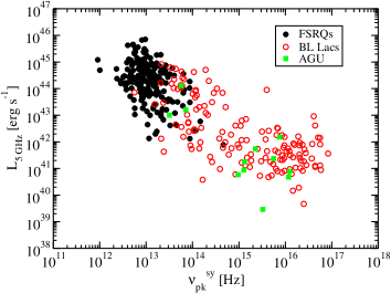
Figure 2: Radio luminosity at 5 GHz versus peak synchrotron frequency for the 2LAC clean sample. Symbols are the same as in Fig. 1.

(abdo10_sed, ) also fit the high energy components of LBAS blazars with a third degree polynomial to determine the peak of the $\gamma$-ray component (presumably from Compton scattering). They found an empirical relation between $\nu_{pk}^{C}$ and the LAT $\gamma$-ray spectral index, $\Gamma_{\gamma}$. We use this relation to determine the peak of the Compton component. Approximately 10% of the 352 sources are also found in the 58-month Swift Burst Alert Telescope (BAT) catalog. For these sources, we extrapolated their BAT and LAT power-laws and found where they intersected. If they intersected within the range 195 keV to 100 MeV we used this location as $\nu_{pk}^{C}$. This allows an improved estimation of $\nu_{pk}^{C}$ over the empirical relation, particularly for those very soft sources, for which this empirical relation is untested. For other sources, the peak was determined from the LAT spectral index and the empirical relation from (abdo10_sed, ). Once the location of $\nu_{pk}^{C}$ is known, either by using the empirical relation or from the BAT-LAT intersection, the luminosity at the peak, $L_{pk}^{C}$, can be estimated by extrapolating the LAT spectral index.

Combining their results with EGRET data, fossati98 made a plot of $\gamma$-ray dominance versus $\nu_{pk}^{sy}$. Using LAT data from the 2LAC, as described above, we make a similar plot, although we use $L_{pk}^{C}$ instead of simply the $\gamma$-ray luminosity. Our results are in Fig. 3. Also note that $A_{C}$ is independent of redshift. Thus we can plot in Fig. 3 an additional 174 sources from the 2LAC clean sample that have well-determined synchrotron bumps but do not have known redshifts. For these sources, the plotted $\nu_{pk}^{sy}$ is a lower limit, since the redshifts are not known. However, it will be larger by only a factor $(1+z)$, i.e., a factor of a few.

We have also computed the correlation coefficients $\rho$ and $\tau$ for $A_{C}$ versus $\nu_{pk}^{sy}$, and the results can be found in Table 1. There is no evidence for a correlation for the FSRQs alone, although the probability that there is no correlation for the BL Lacs alone is very small. For the combined sample of all sources with known $z$, there is essentially zero chance that there is no correlation, similar to the $L_{pk}^{sy}$ versus $\nu_{pk}^{sy}$ correlation. We also computed the coefficients for all sources, including the ones with unknown $z$, computing their $\nu_{pk}^{sy}$ assuming $z=0$ (“all sources 1” in Table 1). We find essentially no chance that the addition of sources with unknown $z$ will explain the correlation when these sources are included. The term $\nu_{pk}^{sy}$ will vary by a factor of a few due to redshift, so we also calculated the coefficients assuming all these sources with unknown $z$ are at $z=0.35$, the average of the BL Lacs with known $z$ (“all sources 2”); and assuming these sources are at $z=4$ (“all sources 3”), which is higher than the maximum redshift of the entire sample (which is $z=3.1$). In each case, there is essentially a 100% chance that an anti-correlation exists. Although the objects without known redshifts could explain the correlation between $L_{pk}^{sy}$ and $\nu_{pk}^{sy}$, it does not appear they can explain the correlation between $A_{C}$ and $\nu_{pk}^{sy}$. This aspect of the blazar sequence seems secure.

The two sources with unknown redshifts in the upper right quadrant of this diagram are 2FGL J0059.2-0151 (1RXS 005916.3-015030) and 2FGL J0912.5+2758 (1RXS J091211.9+27595) with LAT spectral indices of $\Gamma_{\gamma}=1.15\pm 0.36$ and $\Gamma_{\gamma}=1.20\pm 0.37$, respectively. These are the two hardest sources in the 2LAC, and the sources with the largest error bars on their spectral index; only one source in the 2LAC clean sample is fainter than these sources (2FGL J1023.6+2959). They are clearly outliers. Propagating the error on their spectral indices, one finds that they have Compton dominances of $\log_{10}(A_{C})=1.44\pm 1.82$ and $\log_{10}(A_{C})=1.48\pm 1.98$, respectively; they have $A_{C}$ consistent with unity within their error bars, and so are consistent with the “L” shape seen in Fig. 3.

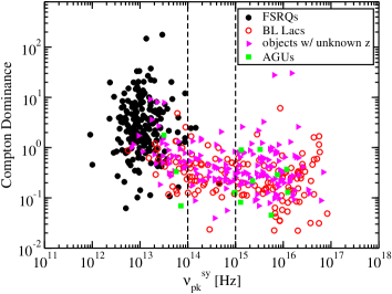
Figure 3: Compton dominance (i.e., $L_{pk}^{C}/L_{pk}^{sy}$) versus peak synchrotron frequency. Symbols are the same as in Figures 1 and 2; additionally, rightward-pointing triangles represent BL Lacs with unknown redshifts, for which $\nu_{pk}^{sy}$ is a lower limit.

III Theoretical Blazar Sequence

We describe a simple model for blazar jet emission. This model is similar to the one presented by boett02_seq . We assume the relativistic jet is dominated by emission from a single zone which is spherical with radius $R^{{}^{\prime}}_{b}$ in its comoving frame, and moving with high relativistic speed $\beta c$ giving it a Lorentz factor $\Gamma=(1-\beta)^{-1/2}$. The jet makes an angle to the line of sight $\theta=\arccos(\mu)$ so that the Doppler factor is $\delta_{\rm D}=[\Gamma(1-\beta\mu)]^{-1}$. Electrons are injected with a power-law distribution given by $Q_{e}(\gamma)=Q_{0}\gamma^{-q}\ H(\gamma;\gamma_{1},\gamma_{2})$. The hard X-ray spectra in some blazars may indicate very hard electron spectra at lower energies (sikora09, ). Although blazars can be quite variable on timescales as short as hours (e.g., abdo09_3c454.3, ) or even minutes (aharonian07_2155, ), we will assume their average or quiescent emission can be described by a steady state solution to the electron continuity equation, where continuous injection is balanced by cooling and escape. We assume an energy-independent escape timescale given by $t_{esc}=\eta R_{b}^{\prime}/c$ where $R_{b}^{\prime}$ is the comoving size of the blob and $\eta$ is a constant $>1$. In this case, where $\gamma_{1}<\gamma_{c}$ (the slow-cooling regime) the electron distribution can be approximated as

$$N_{e}(\gamma)\approx Q_{0}t_{esc}\left\{\begin{array}[]{ll}(\gamma/\gamma_{c})^{-q}&\gamma_{1}<\gamma<\gamma_{c}\\ (\gamma/\gamma_{c})^{-q-1}&\gamma_{c}<\gamma<\gamma_{2}\end{array}\right.\ .$$ (1)

If $\gamma_{c}<\gamma_{1}$, i.e., the fast-cooling regime,

$$N_{e}(\gamma)\approx Q_{0}t_{esc}\left\{\begin{array}[]{ll}(\gamma/\gamma_{1})^{-2}&\gamma_{c}<\gamma<\gamma_{1}\\ (\gamma/\gamma_{1})^{-q-1}&\gamma_{1}<\gamma<\gamma_{2}\end{array}\right.\ .$$ (2)

Here we assume the electrons are cooled by synchrotron emission and Thomson scattering, so that

$$\gamma_{c}=\frac{3m_{e}c^{2}}{4c\sigma_{\rm T}(u^{\prime}_{B}+u^{\prime}_{sy}+\Gamma^{2}u_{ext})t_{esc}}\$$ (3)

is the cooling electron Lorentz factor, where primes denote quantities in the comoving frame of the blob. Here $u^{\prime}_{B}=B^{2}/(8\pi)$ is the magnetic field energy density, $u^{\prime}_{sy,tot}$ is the total synchrotron energy density, and the $u_{ext}$ is the external energy density, assumed to be isotropic in the proper frame of the AGN. The exact nature of the external radiation field is not known, and may not even be the same for all blazars. For a given set of parameters, the nonlinear nature of $u^{\prime}_{sy}$ means that there is not a simple closed form solution for $N_{e}(\gamma)$, and so we solve for $N_{e}(\gamma)$ numerically.

Once $N_{e}(\gamma)$ is known, we use the standard formulae in the $\delta$-approximation (e.g., dermer02, ; finke08_SSC, ; dermer09_book, ) to calculate the synchrotron, SSC, and EC luminosity and energy at their peaks. This assumes the Compton-scattering takes place only in the Thomson regime. We have compared our results with those using the full synchrotron emissivity and Compton cross section, and found good agreement. The Compton dominance ($A_{C}$) is given by the ratio of the peak Compton-scattered component to the peak of the synchrotron component, $A_{C}\equiv\max[L^{EC}_{pk},\ L^{SSC}_{pk}]/L^{sy}_{pk}\approx\max[\delta_{\rm D}^{2}u_{ext},\ u^{\prime}_{sy,pk}]/u^{\prime}_{B}\ ,$ where we have ignored a bolometric correction term $\sim 1$. Note that SSC emission has the same beaming pattern as synchrotron, and thus $L^{SSC}_{pk}/L^{sy}_{pk}$ does not depend on the viewing angle; however, $L^{EC}_{pk}$ does not, and thus $L^{EC}_{pk}/L^{sy}_{pk}$ is dependent of the viewing angle through $\delta_{\rm D}$ (dermer95, ; georgan01, ).

We found we could adequately reproduce the sources in Figures 1 and 3 without changing the power injected in electrons. Instead, we only vary $B$ and $u_{ext}$, assuming $B\propto u_{ext}^{1/4}$, and the angle to the line of sight, $\theta$. Further details can be found in finke12 .

Using the model described above, we reproduce the $L_{pk}^{sy}$ versus $\nu_{pk}^{sy}$ relation as seen in the curves in Fig. 4. At $\lesssim 10^{13}$ Hz (the exact value depends on $\theta$), $\gamma_{c}$ will become less than $\gamma_{1}$, leading to a sharp inflection. By changing the viewing angle, the synchrotron luminosity decreases dramatically, so that almost all of the BL Lacs can be reproduced by this model. Note that this model predicts that there will be sources found with $L_{pk}^{sy}\gtrsim 10^{47}\ \mathrm{erg}\ \mathrm{s}^{-1}$ and $\nu_{pk}^{sy}\gtrsim 10^{15}\ \mathrm{Hz}$, which is relatively unpopulated. This region could be filled in by bright BL Lacs at high $z$, which for which we cannot determine a redshift due to the nonthermal emission washing out their weak emission lines giommi12_selection . Indeed, this region is beginning to be filled in by constraining the redshifts of several BL Lacs (padovani12, ).

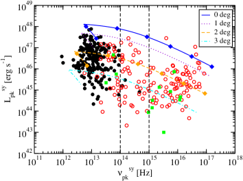
Figure 4: Same as Figure 1, with curves showing our model plotted at various angles, shown in the legend. Along the curves only $B$ and $u_{ext}$ are varyed.

The model curves for $A_{C}$ versus $\nu_{pk}^{sy}$ are plotted in Fig. 5. Again, the model seems to reproduce the 2LAC data well. There is a distinct difference above and below the transition between the Compton component being dominated by SSC and being dominated by EC, at around $\nu_{pk}^{sy}\approx 2\times 10^{15}\ \mathrm{Hz}$ for the $\theta=0$ curve. Note that $A_{C}$ is not dependent on $\theta$ for SSC, although the curve here does shift to lower $\nu_{pk}^{sy}$ due to its dependence on $\theta$. The EC part of the curves, however, are strongly dependent on $\theta$ through $\delta_{\rm D}$. As with Fig. 4, a sharp inflection is seen at lower frequencies ($\nu_{pk}^{sy}\approx 10^{13}\ \mathrm{Hz}$ for $\theta=0$) due to the transition of the peak from being associated with $\gamma_{c}$ to $\gamma_{1}$. Also as with the previous figure, the BL Lacs are well-reproduced, while the FSRQs are not, particularly those with high $A_{C}$. A diversity of $\gamma_{1}$ would clearly allow a widening of this branch, and allow the model to reproduce all of the FSRQs. Alternatively, if the jets of blazars are made up of multiple emitting components with different Lorentz factors, so that at different angles a different jet component would dominate the SED, this could also broaden the sequence and reproduce more objects (meyer11, ).

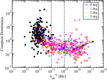
Figure 5: Same as Figure 3 with curves showing our model plotted at various angles, shown in the legend. Along the curves only $B$ and $u_{ext}$ are varyed.

IV Discussion

For blazars, it has been suggested that the peak of the electron distribution ($\gamma_{pk}$) is independent of broad emission line luminosities, $B$, and other properties (giommi12_selection, ). If this were the case, and if the broad lines are the source for external scattering, sources would be found with high $A_{C}$ ($A_{C}\gtrsim$ a few) and and high $\nu_{pk}^{sy}$ ($\nu_{pk}^{sy}\gtrsim 10^{15}\ \mathrm{Hz}$). The redshift is not relevant, since both of these quantities are essentially redshift independent. However, no such sources are found in our sample, including BL Lacs without known redshift (Fig. 5). If $\gamma$ rays are produced by external Compton processes, as seems likely (meyer12, ), there does indeed seem to be a relation between $u_{ext}$ and $\gamma_{pk}$. We have found a simple model that explains this, where $\gamma_{pk}=\max[\gamma_{c},\gamma_{1}]$, where $\gamma_{c}$ is dependent on both $u_{ext}$ and $B$ (Equation [3]). This is quite similar to previous work (e.g., ghisellini98, ; boett02_seq, ), the main different being the dependence of $B$ and $u_{ext}$. This simple model predicts sources will be found with $L_{pk}^{sy}\gtrsim 10^{47}\ \mathrm{erg}\ \mathrm{s}^{-1}$ and $\nu_{pk}^{sy}\gtrsim 10^{15}\ \mathrm{Hz}$ (Fig. 4), when the redshifts of more BL Lacs are determined (unlike ghisellini98, ; boett02_seq, ). These sources should be brighter because they are more highly aligned with our line of sight, rather than intrinsic brightness. ghisellini12_seq also predict that sources will be found in this region, although in their case these sources will be “blue FSRQs”, with the primary emitting region ourside the BLR, assuming in other FSRQs, broad line photons are the external radiation source for Compton scattering.

- (1) M. J. M. Marcha, I. W. A. Browne, C. D. Impey, and P. S. Smith, “Optical spectroscopy and polarization of a new sample of optically bright flat radio spectrum sources,” MNRAS, vol. 281, pp. 425–448, July 1996.
- (2) A. A. Abdo et al., “The Spectral Energy Distribution of Fermi Bright Blazars,” Astrophys. J. , vol. 716, pp. 30–70, June 2010.
- (3) G. Fossati, L. Maraschi, A. Celotti, A. Comastri, and G. Ghisellini, “A unifying view of the spectral energy distributions of blazars,” MNRAS, vol. 299, pp. 433–448, Sept. 1998.
- (4) G. Ghisellini, A. Celotti, G. Fossati, L. Maraschi, and A. Comastri, “A theoretical unifying scheme for gamma-ray bright blazars,” MNRAS, vol. 301, pp. 451–468, Dec. 1998.
- (5) M. Böttcher and C. D. Dermer, “An Evolutionary Scenario for Blazar Unification,” Astrophys. J. , vol. 564, pp. 86–91, Jan. 2002.
- (6) P. Padovani, E. S. Perlman, H. Landt, P. Giommi, and M. Perri, “What Types of Jets Does Nature Make? A New Population of Radio Quasars,” Astrophys. J. , vol. 588, pp. 128–142, May 2003.
- (7) G. Ghisellini and F. Tavecchio, “The blazar sequence: a new perspective,” MNRAS, vol. 387, pp. 1669–1680, July 2008.
- (8) P. Giommi, P. Padovani, M. Perri, H. Landt, and E. Perlman, “Parameter Correlations and Cosmological Properties of BL Lac Objects,” in Blazar Astrophysics with BeppoSAX and Other Observatories (P. Giommi, E. Massaro, & G. Palumbo, ed.), pp. 133–+, 2002.
- (9) P. Padovani, L. Costamante, G. Ghisellini, P. Giommi, and E. Perlman, “BeppoSAX Observations of Synchrotron X-Ray Emission from Radio Quasars,” Astrophys. J. , vol. 581, pp. 895–911, Dec. 2002.
- (10) P. Giommi, S. Piranomonte, M. Perri, and P. Padovani, “The sedentary survey of extreme high energy peaked BL Lacs,” A&A, vol. 434, pp. 385–396, Apr. 2005.
- (11) E. Nieppola, M. Tornikoski, and E. Valtaoja, “Spectral energy distributions of a large sample of BL Lacertae objects,” A&A, vol. 445, pp. 441–450, Jan. 2006.
- (12) L. Chen and J. M. Bai, “Implications for the Blazar Sequence and Inverse Compton Models from Fermi Bright Blazars,” Astrophys. J. , vol. 735, pp. 108–+, July 2011.
- (13) A. A. Abdo et al., “Bright Active Galactic Nuclei Source List from the First Three Months of the Fermi Large Area Telescope All-Sky Survey,” Astrophys. J. , vol. 700, pp. 597–622, July 2009.
- (14) E. T. Meyer, G. Fossati, M. Georganopoulos, and M. L. Lister, “From the Blazar Sequence to the Blazar Envelope: Revisiting the Relativistic Jet Dichotomy in Radio-loud Active Galactic Nuclei,” Astrophys. J. , vol. 740, pp. 98–+, Oct. 2011.
- (15) P. Giommi et al., “Simultaneous Planck, Swift, and Fermi observations of X-ray and -ray selected blazars,” A&A, vol. 541, p. A160, May 2012.
- (16) M. Ackermann et al., “The Second Catalog of Active Galactic Nuclei Detected by the Fermi Large Area Telescope,” Astrophys. J. , vol. 743, p. 171, Dec. 2011.
- (17) A. Rau et al., “BL Lacertae objects beyond redshift 1.3 - UV-to-NIR photometry and photometric redshift for Fermi/LAT blazars,” A&A, vol. 538, p. A26, Feb. 2012.
- (18) P. Giommi, P. Padovani, G. Polenta, S. Turriziani, V. D’Elia, and S. Piranomonte, “A simplified view of blazars: clearing the fog around long-standing selection effects,” MNRAS, vol. 420, pp. 2899–2911, Mar. 2012.
- (19) M. L. Lister et al., “-Ray and Parsec-scale Jet Properties of a Complete Sample of Blazars From the MOJAVE Program,” Astrophys. J. , vol. 742, p. 27, Nov. 2011.
- (20) M. Sikora, Ł. Stawarz, R. Moderski, K. Nalewajko, and G. M. Madejski, “Constraining Emission Models of Luminous Blazar Sources,” Astrophys. J. , vol. 704, pp. 38–50, Oct. 2009.
- (21) A. A. Abdo et al., “Early Fermi Gamma-ray Space Telescope Observations of the Quasar 3C 454.3,” Astrophys. J. , vol. 699, pp. 817–823, July 2009.
- (22) F. Aharonian et al., “An Exceptional Very High Energy Gamma-Ray Flare of PKS 2155-304,” ApJ Letters, vol. 664, pp. L71–L74, Aug. 2007.
- (23) C. D. Dermer and R. Schlickeiser, “Transformation Properties of External Radiation Fields, Energy-Loss Rates and Scattered Spectra, and a Model for Blazar Variability,” Astrophys. J. , vol. 575, pp. 667–686, Aug. 2002.
- (24) J. D. Finke, C. D. Dermer, and M. Böttcher, “Synchrotron Self-Compton Analysis of TeV X-Ray-Selected BL Lacertae Objects,” Astrophys. J. , vol. 686, pp. 181–194, Oct. 2008.
- (25) C. D. Dermer and G. Menon, High Energy Radiation from Black Holes: Gamma Rays, Cosmic Rays, and Neutrinos. 2009.
- (26) C. D. Dermer, “On the Beaming Statistics of Gamma-Ray Sources,” ApJ Letters, vol. 446, pp. L63+, June 1995.
- (27) M. Georganopoulos, J. G. Kirk, and A. Mastichiadis, “The Beaming Pattern and Spectrum of Radiation from Inverse Compton Scattering in Blazars,” Astrophys. J. , vol. 561, pp. 111–117, Nov. 2001.
- (28) J. D. Finke Astrophys. J. , submitted, 2012.
- (29) P. Padovani, P. Giommi, and A. Rau, “The discovery of high-power high synchrotron peak blazars,” MNRAS, vol. 422, p. L48, May 2012.
- (30) E. T. Meyer, G. Fossati, M. Georganopoulos, and M. L. Lister, “Collective Evidence for Inverse Compton Emission from External Photons in High-power Blazars,” ApJ Letters, vol. 752, p. L4, June 2012.
- (31) G. Ghisellini, F. Tavecchio, L. Foschini, T. Sbarrato, G. Ghirlanda, and L. Maraschi, “Blue Fermi Flat Spectrum Radio Quasars,” MNRAS, in press, arXiv:1205.0808, May 2012.