Rigorous asymptotic analysis of buckling of thin-walled cylinders under axial compression

Abstract

Using rigorous constitutive linearization of second variation introduced in [6] we study weak stability of homogeneous deformation of the axially compressed circular cylindrical shell, regarded as a 3-dimensional hyperelastic body. We show that such deformation becomes weakly unstable at the citical load that coincides with value of the bifurcation load in von-Kármán-Donnel shell theory. We also show that the linear bifurcation modes described by the Koiter circle [11] minimize the second variation asymptotically. The key ingredients of our analysis are the asymptoticaly sharp estimates of the Korn constant for cylindrical shells and Korn-like inequalities on components of the deformation gradient tensor in cylindrical coordinates. The notion of buckling equivalence introduced in [6] is developed further and becomes central in this work. A link between features of this theory and sensitivity of the critical load to imprefections of load and shape is conjectured.

1 Introduction

Recent years have seen significant progress in rigorous analysis of dimensionally reduced theories of plates and shells based on $\Gamma$-convergence [3, 16, 4, 12, 13]. In the framework of these theories one must postulate the scaling of energy and the forces apriori, whereby different scaling assumptions lead to different dimensionally reduced plate and shell theories. By contrast [6] has no need for such apriori assumptions, while pursuing a less general goal of identifying a critical load at which the trivial branch of equilibria becomes weakly unstable. This exclusive targeting of the instability without the attempt to capture post-buckling behavior leads to significant technical simplifications in a rigorous analysis of the safe load problem for slender structures. Present work builds on the ideas of [6] and applies them to buckling of a circular cylindrical shell under axial compression.

The asymptotics of the critical buckling load predicted by the sign of the 3-dimensional second variation agrees with the classical value in the shell theory [15, 18, 11]. The displacement variations that minimize the normalized second variation of the energy are single Fourier modes, whose wave numbers lie on Koiter’s circle [11]. Using the notion of buckling equivalence [6] we link the classical variational problem for the buckling load obtained from the shell theory and the rigorous analysis of the sign of the 3-dimensional second variation of the non-linear elastic energy.

The problem of buckling of axially compressed cylindrical shells occupies a special place in engineering. Cylindrical shells are light weight structures with superior load carrying capacity in axial direction as compared to plates of the same thickness. They are ubiquitous in industry. Yet, the classical theoretical value of the buckling load is about 4 to 5 times higher than the one observed in experiments [2]. This is understood as a manifestation of the sensitivity of the buckling load to imperfections of load and shape [1, 17, 19, 5, 20]. The general understanding of the sensitivity of the buckling load to imperfections is via the bifurcation theory applied to von-Kármán-Donnell equations [9, 10, 14, 7]. The subcritical nature of the bifurcation [9, 7], where the load drops sharply at the critical load is responsible for the observed discrepancy between the theoretical and apparent value of the critical load. It is important to note that the formal asymptotics leading to the theoretical value of the critical load gives no indication of the nature of bifurcation and the resultant imperfection sensitivity.

Our approach to buckling of a circular cylindrical shell, along with the rigorous derivation of the classical buckling load, may offer an alternative interpretation of the sensitivity of the critical load to imperfections. Our analysis makes apparent three different asymptotics of the buckling load, only one of which (the one with the largest critical load) is realized in a perfect uniformly axially compressed cylindrical shell. Imprefections of load and shape lead to small perturbations in a trivial branch that are shown to be sufficient to change the asymptotics of the buckling load. While the rigorous analysis requires more work and is left to future studies, we conjecture that the two other buckling loads that are significantly lower that the classical one could lead to a more transparent explanation of imperfection sensitivity.

Recall that a stable configuration $\bm{y}=\bm{y}(\bm{x})$, $\bm{x}\in\Omega\subset\mathbb{R}^{3}$ must be a weak local minimizer of the energy

$$\int_{\Omega}W(\nabla\bm{y})d\bm{x}-\int_{\partial\Omega}(\bm{y},\bm{t}(\bm{x}))dS(\bm{x}),$$

where $W(\bm{F})$ is the energy density function of the body and $\bm{t}(\bm{x})$ is the vector of dead load tractions. The essential non-linearity of buckling comes from the principle of frame indifference $W(\bm{R}\bm{F})=W(\bm{F})$ for all $\bm{R}\in SO(3)$, combined with the assumption of the absence of residual stress $W_{\bm{F}}(\bm{I})=\bm{0}$. For slender bodies these assumptions are fundamental for the computation of the constitutive linearization, which is based on the fact that the stresses are small at every point in the body right up to the buckling point, and therefore, the material response can be linearized locally. The impossibility of the geometric linearization due to the distributed nature of local rotations is the essential feature of slender bodies.

The constitutively linearized problem can be viewed as the variational formulation of the linear eigenvalue problem at the bifurcation point. As such it permits an extra degree of flexibility, as one can replace one variational formulation with an asymptotically equivalent one [6]. This flexibility is used in this paper to simplify and eliminate heavy algebraic calculations for the perfect cylinder.

This paper is organized as follows. In Section 2 we extend the general theory of buckling developed in [6], so that it applies to more general 3-dimensional bodies, including cylindrical shells. We define an equivalence class of functionals characterizing buckling and give criteria for showing that a pair of functionals belongs to the same equivalence class. In Section 3 we discuss the asymptotics of the Korn constant for cylindrical shells. The technical details of the proof are in Appendix A. In Section 4 we prove Korn-like inequalities where the linear strain is bounded in terms of the specific components if the displacement gradient. In Section 5 we compute the compressive part of the constitutively linearized functional whose destabilizing action is ultimately responsible for buckling when the load reaches critical. In Section 6 we apply the general theory of buckling from Section 2 to axially compressed perfect cylindrical shells and derive the formula for the buckling load, as well as a collection of buckling modes parametrized by points on the Koiter’s circle [11]. In Section 7 we show that the more realistic but also more technically challenging boundary conditions, where displacements are prescribed on the top and bottom boundaries of the shell produce exactly the same buckling load. This is achieved by exploiting the massive non-uniqueness of the buckling modes for the the prescribed average vertical displacement boundary conditions of Section 6. In Section 8 we comment on the possibility of the link between the sensitivity to imperfection of the buckling load of a slender structure and the presence of “latent” buckling modes with significantly smaller critical loads.

2 Buckling of slender structures

Here we revisit the general theory of buckling developed in [6]. The theory deals with a sequence of progressively slender domains $\Omega_{h}$ parametrized by a dimensionless parameter $h$. For example, in the case of the cylindrical shell, $h$ is the ratio of cylinder wall thickness to the cylinder radius. We consider a loading program parametrized by the loading parameter $\lambda$ describing the magnitude of the applied tractions $\bm{t}(\bm{x};h,\lambda)=\lambda\bm{t}^{h}(\bm{x})+O(\lambda^{2})$, as $\lambda\to 0$. Here and below $O(\cdot)$ is understood uniformly in $\bm{x}\in\Omega_{h}$ and $h\in[0,h_{0}]$. Two fundamental assumptions need to be made in order for the general theory of buckling to be applicable.

The first fundamental assumption requires the existence of the family of equilibrium deformations $\bm{y}(\bm{x};h,\lambda)$, corresponding to the applied loads $\bm{t}(\bm{x};h,\lambda)$ and satisfying the imposed boundary conditions, for any $h\in[0,h_{0}]$ and $\lambda\in[0,\lambda_{0}]$, where $h_{0}>0$ and $\lambda_{0}>0$ are some constants. Such a family of equilibria will be called a “trivial branch”. Neither uniqueness nor its stability is assumed.

The second fundamental assumption is the absence of “bending modes” in the trivial branch. Here we use the term “bending” loosely to indicate any response in which the strain to stress ratio becomes infinitely large as $h\to 0$ even for small applied stress. Formally we assume that the trivial branch lies uniformly close to the linearly elastic response:

$$\sup_{0\leq h\leq h_{0}}\|\nabla\bm{y}(\bm{x};h,\lambda)-\bm{I}-\lambda\nabla\bm{u}^{h}(\bm{x})\|_{L^{\infty}(\Omega_{h})}\leq C\lambda^{2},\qquad\bm{u}^{h}(\bm{x})=\left.\displaystyle\frac{\partial\bm{y}(\bm{x};h,\lambda)}{\partial\lambda}\right|_{\lambda=0},$$ (2.1)

when $0\leq\lambda\leq\lambda_{0}$ and the constant $C$ is independent of $h$.

In [6] we have defined the notion of the near-flip buckling when for any $h\in[0,h_{0}]$ the trivial branch becomes unstable for $\lambda>\lambda(h)$, where $\lambda(h)\to 0$, as $h\to 0$. This happens because it becomes energetically more advantageous to activate bending modes rather than store more compressive stress.

In hyperelasticity the trivial branch $\bm{y}(\bm{x};h,\lambda)$ is a critical point of the energy functional

$${\mathcal{E}}(\bm{y})=\int_{\Omega_{h}}W(\nabla\bm{y})d\bm{x}-\int_{\partial\Omega_{h}}(\bm{t}(\bm{x};h,\lambda),\bm{y})dS.$$ (2.2)

In general we restrict $\bm{y}$ to an affine subspace of $W^{1,\infty}(\Omega_{h};\mathbb{R}^{3})$ given by

$$\bm{y}\in\overline{\bm{y}}(\bm{x};h,\lambda)+V_{h}^{\circ},$$ (2.3)

where $V_{h}^{\circ}$ is a linear subspace of $W^{1,\infty}(\Omega_{h};\mathbb{R}^{3})$ that contains $W_{0}^{1,\infty}(\Omega_{h};\mathbb{R}^{3})$ and does not depend on the loading parameter $\lambda$. The given function $\overline{\bm{y}}(\bm{x};h,\lambda)\in W^{1,\infty}(\Omega_{h};\mathbb{R}^{3})$ describes the Dirichlet part of the boundary conditions, while the traction vector $\bm{t}(\bm{x};h,\lambda)$ describes the Neumann-part.

The equilibrium equations and the boundary conditions satisfied by the trivial branch $\bm{y}(\bm{x};h,\lambda)$ can be written explicitly only in the weak form:

$$\int_{\Omega_{h}}(W_{\bm{F}}(\nabla\bm{y}(\bm{x};h,\lambda)),\nabla\bm{\phi})d\bm{x}-\int_{\partial\Omega_{h}}(\bm{t}(\bm{x};h,\lambda),\bm{\phi})dS=0$$ (2.4)

for every $\bm{\phi}\in V_{h}$, where $V_{h}$ is a closure of $V_{h}^{\circ}$ in $W^{1,2}(\Omega_{h};\mathbb{R}^{3})$. Differentiating (2.4) in $\lambda$ at $\lambda=0$, which is allowed due to (2.1), we obtain

$$\int_{\Omega_{h}}(\mathsf{L}_{0}\nabla\bm{u}^{h}(\bm{x}),\nabla\bm{\phi})d\bm{x}-\int_{\partial\Omega_{h}}(\bm{t}^{h}(\bm{x}),\bm{\phi})dS=0,\qquad\bm{\phi}\in V_{h}$$ (2.5)

where $\mathsf{L}_{0}=W_{\bm{F}\bm{F}}(\bm{I})$.

The energy density $W(\bm{F})$ satisfies two fundamental assumptions:

• Absence of prestress: $W_{\bm{F}}(\bm{I})=\bm{0}$;

• Frame indifference: $W(\bm{F}\bm{R})=W(\bm{F})$ for every $\bm{R}\in SO(3)$;

• Positive semidefiniteness property $(\mathsf{L}_{0}\bm{\xi},\bm{\xi})\geq 0$ for any $\bm{\xi}\in\mathbb{R}^{3\times 3}$;

• Non-degeneracy $(\mathsf{L}_{0}\bm{\xi},\bm{\xi})=0$ if and only if $\bm{\xi}^{T}=-\bm{\xi}$.

By the properties (P3)–(P4) of $\mathsf{L}_{0}$, there exists $\alpha_{\mathsf{L}_{0}}>0$, such that

$$(\mathsf{L}_{0}\bm{\xi},\bm{\xi})\geq\alpha_{\mathsf{L}_{0}}|\bm{\xi}_{\rm sym}|^{2},\qquad\bm{\xi}_{\rm sym}=\displaystyle\frac{1}{2}(\bm{\xi}+\bm{\xi}^{T}).$$ (2.6)

The buckling is detected by the second variation of energy

$$\delta^{2}{\mathcal{E}}(\bm{\phi};h,\lambda)=\int_{\Omega_{h}}(W_{\bm{F}\bm{F}}(\nabla\bm{y}(\bm{x};h,\lambda))\nabla\bm{\phi},\nabla\bm{\phi})d\bm{x}.$$

The second variation is always non negative, when $0<\lambda<\lambda(h)$ and can become negative for some choice of the admissible variation $\bm{\phi}\in V_{h}$, when $\lambda>\lambda(h)$. It was understood in [6] that this failure of weak stability is due to the properties (P1)–(P4) of $W(\bm{F})$ and is intimately related to flip instability in soft device. It was shown in [6] that in an “almost soft” device the critical load could be captured (under some assumptions) by the constitutively linearized second variation

$$\delta^{2}{\mathcal{E}}_{cl}(\bm{\phi};h,\lambda)=\int_{\Omega_{h}}\{(\mathsf{L}_{0}e(\bm{\phi}),e(\bm{\phi}))-\lambda(\bm{\sigma}_{h},\nabla\bm{\phi}^{T}\nabla\bm{\phi})\}d\bm{x},$$ (2.7)

where

$$\bm{\sigma}_{h}(\bm{x})=-\mathsf{L}_{0}e(\bm{u}^{h}(\bm{x})),\qquad e(\bm{u})=\displaystyle\frac{1}{2}(\nabla\bm{u}+(\nabla\bm{u})^{T}).$$ (2.8)

Observe, that $\bm{\sigma}^{h}$ is minus the linear stress in the body. This notation is convenient when we are dealing exclusively with compressive stresses. The larger the stress, the more compressive the load. Let

$${\mathcal{A}}_{h}=\left\{\bm{\phi}\in V_{h}:\int_{\Omega_{h}}(\bm{\sigma}_{h},\nabla\bm{\phi}^{T}\nabla\bm{\phi})d\bm{x}>0\right\}$$ (2.9)

be the set of all destabilizing variations (see (2.7)).

Definition 2.1.

We say that the loading is weakly compressive if there exists $h_{0}>0$ so that ${\mathcal{A}}_{h}\not=\emptyset$, for all $h<h_{0}$.

If the stress is not weakly compressive, then both terms in (2.7) are non-negative for all $\bm{\phi}$ and the instability is clearly impossible. If the loading is weakly compressive then the two terms in (2.7) have opposite signs for all variations $\bm{\phi}\in{\mathcal{A}}_{h}$. The linearized second variation can then become negative for sufficiently large $\lambda$. However, this does not immediately imply negativity of the second variation $\delta^{2}{\mathcal{E}}(\bm{\phi};h,\lambda)$. To examine the sign of the second variation we consider the function

$$m^{*}(h,\lambda)=\inf_{\bm{\phi}\in{\mathcal{A}}_{h}}\frac{\delta^{2}{\mathcal{E}}(\bm{\phi};h,\lambda)}{\int_{\Omega_{h}}(\bm{\sigma}_{h},\nabla\bm{\phi}^{T}\nabla\bm{\phi})d\bm{x}}$$

that measures reserve of stability in the trivial branch. Negative values of $m^{*}(h,\lambda)$ signal instability. The functional $m^{*}(h,\lambda)$ is based on the representation of the buckling load as a generalized Korn constant in [6].

Remark 2.2.

The theory of buckling of slender bodies in [6] is based on the analysis of the function

$$m(h,\lambda)=\inf_{\bm{\phi}\in V_{h}}\frac{\delta^{2}{\mathcal{E}}(\bm{\phi};h,\lambda)}{\|\nabla\bm{\phi}\|^{2}}.$$

We will see that for the axially compressed cylindrical shell

$$\int_{\Omega_{h}}(\bm{\sigma}_{h},\nabla\bm{\phi}_{h}^{T}\nabla\bm{\phi}_{h})d\bm{x}=o(\|\nabla\bm{\phi}_{h}\|^{2})$$ (2.10)

for the minimizer $\bm{\phi}_{h}$ in $m^{*}(h,\lambda(h))$. Therefore,

$$M(p)=\lim_{h\to 0}\frac{m(h,p\lambda(h))}{\lambda(h)}=0,$$

and the link between $\delta^{2}{\mathcal{E}}(\bm{\phi};h,\lambda)$ and $\delta^{2}{\mathcal{E}}_{cl}(\bm{\phi};h,\lambda)$ cannot be ascertained. In this paper we will show that replacing $m(h,\lambda)$ with $m^{*}(h,\lambda)$ permits to establish the required link. We also observe that the distinction between $m(h,\lambda)$ and $m^{*}(h,\lambda)$ is essentially 3-dimensional, since, as we have shown in [6],

$$\int_{\Omega_{h}}(\bm{\sigma}_{h},\nabla\bm{\phi}_{h}^{T}\nabla\bm{\phi}_{h})d\bm{x}\sim\int_{\Omega_{h}}\displaystyle\frac{1}{2}(\mathrm{Tr}\,\bm{\sigma}_{h})|\nabla\bm{\phi}_{h}|^{2}d\bm{x}.$$

Definition 2.3.

We say that $\lambda(h)$ is the buckling load if

$$\lambda(h)=\inf\{\lambda>0:m^{*}(h,\lambda)<0\}.$$

We say that $\{\bm{\phi}_{h}\in{\mathcal{A}}_{h}:h\in(0,h_{0})\}$ is a buckling mode if

$$\lim_{h\to 0}\frac{\delta^{2}{\mathcal{E}}(\bm{\phi}_{h};h,\lambda(h))}{\lambda(h)\int_{\Omega_{h}}(\bm{\sigma}_{h},\nabla\bm{\phi}_{h}^{T}\nabla\bm{\phi}_{h})d\bm{x}}=0,$$

where $\lambda(h)$ is the buckling load.

Definition 2.4.

We will call the loading strongly compressive, if $\lambda(h)\to 0$, as $h\to 0$.

According to (2.7), strongly compressive loads imply existence of variations $\bm{\phi}\in{\mathcal{A}}_{h}$ for which the measure of compressiveness

$$\mathfrak{C}_{h}(\bm{\phi})=\int_{\Omega_{h}}(\bm{\sigma}_{h},\nabla\bm{\phi}^{T}\nabla\bm{\phi})d\bm{x}$$

is much larger than the measure of stability

$$\mathfrak{S}_{h}(\bm{\phi})=\int_{\Omega_{h}}(\mathsf{L}_{0}e(\bm{\phi}),e(\bm{\phi}))d\bm{x}.$$

In particular, the body $\Omega_{h}$ has to be slender in the sense that the Korn constant

$$K(V_{h})=\inf_{\bm{\phi}\in V_{h}}\frac{\|e(\bm{\phi})\|^{2}}{\|\nabla\bm{\phi}\|^{2}}$$ (2.11)

is infinitesimal $K(V_{h})\to 0$, as $h\to 0$.

The notion of the buckling mode in Definition 2.3 suggests an extension of the notion of buckling equivalence to include buckling modes in addition to buckling loads.

Definition 2.5.

Assume $J(h,\bm{\phi})$ is a variational functional defined on ${\mathcal{B}}_{h}\subset{\mathcal{A}}_{h}$. We say that the pair $({\mathcal{B}}_{h},J(h,\bm{\phi}))$ characterizes buckling if the following three conditions are satisfied

1. Characterization of the buckling load:

   $$\lim_{h\to 0}\frac{\widehat{\lambda}(h)}{\lambda(h)}=1,$$

   where $\lambda(h)$ is the buckling load and

   $$\widehat{\lambda}(h)=\inf_{\bm{\phi}\in{\mathcal{B}}_{h}}J(h,\bm{\phi}).$$

2. Characterization of the buckling mode: If $\bm{\phi}_{h}\in{\mathcal{B}}_{h}$ is a buckling mode, then

   $$\lim_{h\to 0}\frac{J(h,\bm{\phi}_{h})}{\widehat{\lambda}(h)}=1.$$ (2.12)

3. Faithful representation of the buckling mode: If $\bm{\phi}_{h}\in{\mathcal{B}}_{h}$ satisfies (2.12) then it is a buckling mode.

We remark that by Definition 2.3 of the buckling mode the pair $({\mathcal{A}}_{h},\mathfrak{J}(h,\bm{\phi}))$ characterizes buckling, where

$$\mathfrak{J}(h,\bm{\phi})=\lambda(h)+\frac{\delta^{2}{\mathcal{E}}(\bm{\phi};h,\lambda(h))}{\mathfrak{C}_{h}(\bm{\phi})}.$$

We envision two ways in which the analysis of buckling can be simplified. One is the simplification of the functional $\mathfrak{J}(h,\bm{\phi})$. The other is replacing the space of all admissible functions ${\mathcal{A}}_{h}$ with a much smaller space ${\mathcal{B}}_{h}$. For example, we may want to use a specific ansatz, like the Kirchhoff ansatz in buckling of rods and plates. According to Definition 2.5 the simplified functional $J(h,\bm{\phi})$, restricted to the ansatz ${\mathcal{B}}_{h}$ will capture the asymptotics of the buckling load and at least one buckling mode. It is in principle conceivable, that there are other buckling modes, not contained in ${\mathcal{B}}_{h}$. However, we believe that such a situation is non-generic. Even in this non-generic situation our approach would allow to capture all geometrically distinct buckling modes, if one can identify the ansatz ${\mathcal{B}}_{h}$ for each of them.

It is an elementary observation that the only requirement we need to place on the ansatz ${\mathcal{B}}_{h}$ is that it must contain a buckling mode.

Lemma 2.6.

Suppose the pair $({\mathcal{B}}_{h},J(h,\bm{\phi}))$ characterizes buckling. Let ${\mathcal{C}}_{h}\subset{\mathcal{B}}_{h}$ be such that it contains a buckling mode. Then the pair $({\mathcal{C}}_{h},J(h,\bm{\phi}))$ also characterizes buckling.

Proof.

Let

$$\widehat{\lambda}(h)=\inf_{\bm{\phi}\in{\mathcal{B}}_{h}}J(h,\bm{\phi}),\qquad\widetilde{\lambda}(h)=\inf_{\bm{\phi}\in{\mathcal{C}}_{h}}J(h,\bm{\phi}).$$

Then, clearly, $\widetilde{\lambda}(h)\geq\widehat{\lambda}(h)$. By assumption there exists a buckling mode $\bm{\phi}_{h}\in{\mathcal{C}}_{h}\subset{\mathcal{B}}_{h}$. Therefore,

$$\mathop{\overline{\lim}}_{h\to 0}\frac{\widetilde{\lambda}(h)}{\widehat{\lambda}(h)}\leq\lim_{h\to 0}\frac{J(h,\bm{\phi}_{h})}{\widehat{\lambda}(h)}=1,$$

since the pair $({\mathcal{B}}_{h},J(h,\bm{\phi}))$ characterizes buckling. Hence

$$\lim_{h\to 0}\frac{\widetilde{\lambda}(h)}{\widehat{\lambda}(h)}=1,$$ (2.13)

and part (a) of Definition 2.5 is established.

If $\bm{\phi}_{h}\in{\mathcal{C}}_{h}\subset{\mathcal{B}}_{h}$ is a buckling mode then

$$\lim_{h\to 0}\frac{J(h,\bm{\phi}_{h})}{\widehat{\lambda}(h)}=1,$$

since the pair $({\mathcal{B}}_{h},J(h,\bm{\phi}))$ characterizes buckling. Part (b) now follows from (2.13).

Finally, if $\bm{\phi}_{h}\in{\mathcal{C}}_{h}$ satisfies

$$\lim_{h\to 0}\frac{J(h,\bm{\phi}_{h})}{\widetilde{\lambda}(h)}=1,$$

then, $\bm{\phi}_{h}\in{\mathcal{B}}_{h}$ and by (2.13) we also have

$$\lim_{h\to 0}\frac{J(h,\bm{\phi}_{h})}{\widehat{\lambda}(h)}=1.$$

Therefore, $\bm{\phi}_{h}$ is a buckling mode, since, by assumption the pair $({\mathcal{B}}_{h},J(h,\bm{\phi}))$ characterizes buckling. The Lemma is proved now. ∎

If we replace the second variation $\delta^{2}{\mathcal{E}}(\bm{\phi};h,\lambda)$ with the constitutively linearized second variation (2.7) in the functional $\mathfrak{J}(h,\bm{\phi})$, we will obtain the functional

$$\mathfrak{K}(h,\bm{\phi})=\frac{\int_{\Omega_{h}}(\mathsf{L}_{0}e(\bm{\phi}),e(\bm{\phi}))d\bm{x}}{\int_{\Omega_{h}}(\bm{\sigma}_{h},\nabla\bm{\phi}^{T}\nabla\bm{\phi})d\bm{x}}=\frac{\mathfrak{S}_{h}(\bm{\phi})}{\mathfrak{C}_{h}(\bm{\phi})},$$ (2.14)

which first appeared in [6] where it was shown that the buckling load can be regarded as a generalized Korn constant

$$\widehat{\lambda}(h)=\inf_{\bm{\phi}\in{\mathcal{A}}_{h}}\mathfrak{K}(h,\bm{\phi}).$$ (2.15)

Unfortunately the sufficient conditions for buckling equivalence established in [6] fail to guarantee the validity of constitutive linearization in the case of the axially compressed thin-walled cylinder for reasons explained in Remark 2.2. Our next theorem proves buckling equivalence and also shows that the constitutively linearized functional $\mathfrak{K}(h,\bm{\phi})$ captures the buckling mode as well.

Theorem 2.7 (Asymptotics of the critical load).

Suppose that the Korn constant $K(V_{h})$ defined by (2.11) satisfies

$$\lim_{h\to 0}K(V_{h})=0,\qquad\lim_{h\to 0}\frac{\widehat{\lambda}(h)^{2}}{K(V_{h})}=0.$$ (2.16)

Then the pair $({\mathcal{A}}_{h},\mathfrak{K}(h,\bm{\phi}))$ characterizes buckling in the sense of Definition 2.5.

Proof.

The theorem is proved by means of the basic estimate, which is a simple modification of the estimates in [6] used in the derivation of the formula for $\delta^{2}{\mathcal{E}}_{cl}(\bm{\phi};h,\lambda)$:

Lemma 2.8.

Suppose $\bm{y}(\bm{x};h,\lambda)$ satisfies (2.1) and $W(\bm{F})$ has the properties (P1)–(P2). Then

$$\left|\delta^{2}{\mathcal{E}}(\bm{\phi};h,\lambda)-\delta^{2}{\mathcal{E}}_{cl}(\bm{\phi};h,\lambda)\right|\leq C(\lambda\|e(\bm{\phi})\|\|\nabla\bm{\phi}\|+\lambda^{2}\|\nabla\bm{\phi}\|^{2}).$$ (2.17)

Proof.

According to the frame indifference property (P2), $W(\bm{F})=\widehat{W}(\bm{F}^{T}\bm{F})$. Differentiating this formula twice we obtain

$$(W_{\bm{F}\bm{F}}(\bm{F})\bm{\xi},\bm{\xi})=4(\widehat{W}_{\bm{C}\bm{C}}(\bm{C})(\bm{F}^{T}\bm{\xi}),\bm{F}^{T}\bm{\xi})+2(\widehat{W}_{\bm{C}}(\bm{C})\bm{\xi}^{T}\bm{\xi}),\qquad\bm{C}=\bm{F}^{T}\bm{F}.$$

We make the following estimate

$$|(\widehat{W}_{\bm{C}\bm{C}}(\bm{C})(\bm{F}^{T}\bm{\xi}),\bm{F}^{T}\bm{\xi})-(\widehat{W}_{\bm{C}\bm{C}}(\bm{I})\bm{\xi},\bm{\xi})|\leq|(\widehat{W}_{\bm{C}\bm{C}}(\bm{C})(\bm{F}^{T}-\bm{I})\bm{\xi},(\bm{F}^{T}-\bm{I})\bm{\xi})|+$$

$$|((\widehat{W}_{\bm{C}\bm{C}}(\bm{C})-\widehat{W}_{\bm{C}\bm{C}}(\bm{I}))\bm{\xi},\bm{\xi})|+2|(\widehat{W}_{\bm{C}\bm{C}}(\bm{C})\bm{\xi},(\bm{F}^{T}-\bm{I})\bm{\xi})|$$

When $\bm{F}$ is uniformly bounded we obtain

$$|(\widehat{W}_{\bm{C}\bm{C}}(\bm{C})(\bm{F}^{T}\bm{\xi}),\bm{F}^{T}\bm{\xi})-(\widehat{W}_{\bm{C}\bm{C}}(\bm{I})\bm{\xi},\bm{\xi})|\leq C\left(|\bm{F}-\bm{I}|^{2}|\bm{\xi}|^{2}+|\bm{C}-\bm{I}||\bm{\xi}_{\rm sym}|^{2}+|\bm{F}-\bm{I}||\bm{\xi}_{\rm sym}||\bm{\xi}|\right).$$

Similarly,

$$|(\widehat{W}_{\bm{C}}(\bm{C})-\widehat{W}_{\bm{C}\bm{C}}(\bm{I})(\bm{C}-\bm{I}),\bm{\xi}^{T}\bm{\xi})|\leq C|\bm{C}-\bm{I}|^{2}|\bm{\xi}|^{2}$$

When $\bm{F}=\nabla\bm{y}(\bm{x};h,\lambda)$ and $\bm{\xi}=\nabla\bm{\phi}$ we obtain, taking into account (2.1), that

$$|\bm{F}-\bm{I}|\leq C\lambda,\qquad|\bm{C}-\bm{I}|\leq C\lambda.$$

The estimate (2.17) now follows from the formulas

$$4\widehat{W}_{\bm{C}\bm{C}}(\bm{I})=W_{\bm{F}\bm{F}}(\bm{I})=\mathsf{L}_{0},\qquad|\bm{C}-\bm{I}-2\lambda e(\bm{u}^{h})|\leq C\lambda^{2}.$$

∎

Let us show that for any $\epsilon>0$ there exists $h(\epsilon)>0$, so that for all $h<h(\epsilon)$ there exists $\bm{\phi}_{h}\in{\mathcal{A}}_{h}$, such that $\delta^{2}{\mathcal{E}}(\bm{\phi}_{h};h,\widehat{\lambda}(h)(1+2\epsilon))<0$. In that case we will be able to conclude that $\lambda(h)\leq\widehat{\lambda}(h)(1+2\epsilon)$ for any $h<h(\epsilon)$. For any fixed $\epsilon$ and any $h>0$ (for which ${\mathcal{A}}_{h}$ is non-empty) there exists $\bm{\phi}_{h}\in{\mathcal{A}}_{h}$ such that

$$\mathfrak{S}_{h}(\bm{\phi}_{h})\leq\widehat{\lambda}(h)(1+\epsilon)\mathfrak{C}_{h}(\bm{\phi}_{h}),$$ (2.18)

thus, putting $\lambda=\lambda_{\epsilon}(h)=\widehat{\lambda}(h)(1+2\epsilon)$ and $\bm{\phi}=\bm{\phi}_{h}$ in (2.17) and utilizing (2.18) we get,

$$\delta^{2}{\mathcal{E}}(\bm{\phi}_{h};h,\lambda_{\epsilon}(h))\leq-\frac{\epsilon}{(1+\epsilon)}\mathfrak{S}_{h}(\bm{\phi}_{h})+C(\widehat{\lambda}(h)\|e(\bm{\phi}_{h})\|\|\nabla\bm{\phi}_{h}\|+\widehat{\lambda}(h)^{2}\|\nabla\bm{\phi}_{h}\|^{2}).$$

By (2.6) we obtain

$$\mathfrak{S}_{h}(\bm{\phi}_{h})\geq\alpha_{\mathsf{L}_{0}}\|e(\bm{\phi}_{h})\|^{2}.$$ (2.19)

Now, by the Korn inequality we obtain

$$\delta^{2}{\mathcal{E}}(\bm{\phi}_{h};h,\lambda_{\epsilon}(h))\leq\left(-\frac{\epsilon\alpha_{L_{0}}}{(1+\epsilon)}+C\left(\frac{\widehat{\lambda}(h)}{\sqrt{K(V_{h})}}+\frac{\widehat{\lambda}(h)^{2}}{K(V_{h})}\right)\right)\|e(\bm{\phi}_{h})\|^{2},$$

We now see that due to (2.16) we have $\delta^{2}{\mathcal{E}}(\bm{\phi}_{h};h,\lambda_{\epsilon}(h))<0$ for sufficiently small $h$.

Now, let us show that for any $\epsilon>0$ there exists $h(\epsilon)>0$, so that for any $h<h(\epsilon)$, any $0<\lambda\leq\widehat{\lambda}(h)(1-\epsilon)$ and any $\bm{\phi}\in{\mathcal{A}}_{h}$ we have $\delta^{2}{\mathcal{E}}(\bm{\phi};h,\lambda)>0$. Indeed, using (2.17) and the generalized Korn inequality

$$\mathfrak{S}_{h}(\bm{\phi})\geq\widehat{\lambda}(h)\mathfrak{C}_{h}(\bm{\phi})$$

we estimate for $0<\lambda\leq\widehat{\lambda}(h)(1-\epsilon)$

$$\delta^{2}{\mathcal{E}}(\bm{\phi};h,\lambda)\geq\epsilon\mathfrak{S}_{h}(\bm{\phi})-|C|(\widehat{\lambda}(h)\|e(\bm{\phi})\|\|\nabla\bm{\phi}\|+\widehat{\lambda}(h)^{2}\|\nabla\bm{\phi}\|^{2})$$

Using (2.19) and the Korn inequality we conclude that

$$\delta^{2}{\mathcal{E}}(\bm{\phi};h,\lambda)\geq\left(\epsilon\alpha_{L_{0}}-C\left(\frac{\widehat{\lambda}(h)}{\sqrt{K(V_{h})}}+\frac{\widehat{\lambda}(h)^{2}}{K(V_{h})}\right)\right)\|e(\bm{\phi})\|^{2}.$$

We now see that $\delta^{2}{\mathcal{E}}(\bm{\phi};h,\lambda)>0$ for sufficiently small $h$, which means that $\lambda(h)\geq\widehat{\lambda}(h)(1-\epsilon)$. Therefore, part (a) of the theorem is proved.

We will now establish part (b). Assume now that $\bm{\phi}_{h}$ is a buckling mode. Then $\alpha_{h}\to 0$, as $h\to 0$, where

$$\alpha_{h}=\frac{\delta^{2}{\mathcal{E}}(\bm{\phi}_{h};h,\lambda(h))}{\lambda(h)\mathfrak{C}_{h}(\bm{\phi}_{h})}.$$

Observe that by virtue of $(a)$, the condition (2.16) holds for $\widehat{\lambda}(h)$ replaced by $\lambda(h),$ therefore by (2.16) and by the Korn inequality,

$$\mathop{\overline{\lim}}_{h\to 0}\frac{\lambda(h)\|e(\bm{\phi}_{h})\|\|\nabla\bm{\phi}_{h}\|}{\mathfrak{S}_{h}(\bm{\phi}_{h})}\leq\mathop{\overline{\lim}}_{h\to 0}\frac{\lambda(h)\|e(\bm{\phi}_{h})\|\|\nabla\bm{\phi}_{h}\|}{\alpha_{L_{0}}\|e(\bm{\phi}_{h})\|^{2}}\leq\mathop{\overline{\lim}}_{h\to 0}\frac{\lambda(h)}{\alpha_{L_{0}}\sqrt{K(V_{h})}}=0,$$ (2.20)

and similarly

$$\lim_{h\to 0}\frac{\lambda(h)^{2}\|\nabla\bm{\phi}_{h}\|^{2}}{\mathfrak{S}_{h}(\bm{\phi}_{h})}=0.$$ (2.21)

Let us substitute $\bm{\phi}=\bm{\phi}_{h}$ and $\lambda=\lambda(h)$ into (2.17) and divide by $\mathfrak{S}_{h}(\bm{\phi}_{h})$. Using (2.20) and (2.21) we obtain

$$\lim_{h\to 0}\left|1-\frac{\lambda(h)}{\mathfrak{K}(h,\bm{\phi}_{h})}-\frac{\delta^{2}{\mathcal{E}}(\bm{\phi}_{h};h,\lambda(h))}{\mathfrak{S}_{h}(\bm{\phi}_{h})}\right|=0.$$

We now use $\alpha_{h}$ to eliminate $\delta^{2}{\mathcal{E}}$:

$$\frac{\delta^{2}{\mathcal{E}}(\bm{\phi}_{h};h,\lambda(h))}{\mathfrak{S}_{h}(\bm{\phi}_{h})}=\frac{\alpha_{h}\lambda(h)}{\mathfrak{K}(h,\bm{\phi}_{h})}.$$

Therefore,

$$\lim_{h\to 0}\frac{(1+\alpha_{h})\lambda(h)}{\mathfrak{K}(h,\bm{\phi}_{h})}=1.$$

Recalling that $\alpha_{h}\to 0$, as $h\to 0$ we conclude that

$$\lim_{h\to 0}\frac{\lambda(h)}{\mathfrak{K}(h,\bm{\phi}_{h})}=1,$$

and part (b) follows via part (a).

Let us prove part (c). Let $\bm{\phi}_{h}$ satisfy (2.12). Then, by part (a), $\beta_{h}\to 0$, as $h\to 0$, where

$$\beta_{h}=\frac{\mathfrak{K}(h,\bm{\phi}_{h})}{\lambda(h)}-1.$$

Therefore,

$$\lambda(h)\mathfrak{C}_{h}(\bm{\phi}_{h})=\frac{1}{1+\beta_{h}}\mathfrak{S}_{h}(\bm{\phi}_{h}).$$ (2.22)

Let us substitute $\bm{\phi}=\bm{\phi}_{h}$ and $\lambda=\lambda(h)$ into (2.17) and divide by $\lambda(h)\mathfrak{C}_{h}(\bm{\phi}_{h})$ to obtain (using 2.22)

$$\left|\frac{\delta^{2}{\mathcal{E}}(\bm{\phi}_{h};h,\lambda(h))}{\lambda(h)\mathfrak{C}_{h}(\bm{\phi}_{h})}-\beta_{h}\right|\leq\frac{C(1+\beta_{h})(\lambda(h)\|e(\bm{\phi}_{h})\|\|\nabla\bm{\phi}_{h}\|+\lambda(h)^{2}\|\nabla\bm{\phi}_{h}\|^{2})}{\mathfrak{S}_{h}(\bm{\phi}_{h})}.$$ (2.23)

Note that (2.20) and (2.21) continue to hold for any $\bm{\phi}_{h}\in{\mathcal{A}}_{h},$. Thus (2.23) implies

$$\lim_{h\to 0}\frac{\delta^{2}{\mathcal{E}}(\bm{\phi}_{h};h,\lambda(h))}{\lambda(h)\mathfrak{C}_{h}(\bm{\phi}_{h})}=0,$$

therefore $\bm{\phi}_{h}$ is a buckling mode. ∎

The passage from the second variation of the trivial branch to the constitutively linearized functional $\mathfrak{K}(h,\bm{\phi})$ is an important simplification. However, in specific problems we might want to simplify the functional $\mathfrak{K}(h,\bm{\phi})$ even further. For that reason we want to establish general criteria for the validity of replacing one functional that characterizes buckling by another. Behind this flexibility is the equivalence relation on the space of functionals.

Definition 2.9.

Two pairs $({\mathcal{B}}_{h},J_{1}(h,\bm{\phi}))$ and $({\mathcal{B}}_{h},J_{2}(h,\bm{\phi}))$ are called buckling equivalent if the pair $({\mathcal{B}}_{h},J_{1}(h,\bm{\phi}))$ characterizes buckling if and only if $({\mathcal{B}}_{h},J_{2}(h,\bm{\phi}))$ does.

The notion of B-equivalence was introduced in [6] on the set of functions $m(h,\lambda)$ in order to capture buckling load by means of constitutive linearization. Definition 2.9 extends the idea of buckling equivalence to functionals in order to capture buckling modes in addition to buckling loads.

Theorem 2.10 below gives a convenient criterion of buckling equivalence.

Theorem 2.10 (Buckling equivalence).

If either

$$\lim_{h\to 0}\lambda(h)\sup_{\bm{\phi}\in{\mathcal{B}}_{h}}\left|\frac{1}{J_{1}(h,\bm{\phi})}-\frac{1}{J_{2}(h,\bm{\phi})}\right|=0,$$ (2.24)

or

$$\lim_{h\to 0}\displaystyle\frac{1}{\lambda(h)}\sup_{\bm{\phi}\in{\mathcal{B}}_{h}}|J_{1}(h,\bm{\phi})-J_{2}(h,\bm{\phi})|=0,$$ (2.25)

then the pairs $({\mathcal{B}}_{h},J_{1}(h,\bm{\phi}))$ and $({\mathcal{B}}_{h},J_{2}(h,\bm{\phi}))$ are buckling equivalent in the sense of Definition 2.9.

Proof.

Let us introduce the notation

$$\widehat{\lambda}_{i}(h)=\inf_{\bm{\phi}\in{\mathcal{B}}_{h}}J_{i}(h,\bm{\phi}),\quad i=1,2.$$

$$\delta_{1}(h)=\lambda(h)\sup_{\bm{\phi}\in{\mathcal{B}}_{h}}\left|\frac{1}{J_{1}(h,\bm{\phi})}-\frac{1}{J_{2}(h,\bm{\phi})}\right|.$$

$$\delta_{2}(h)=\displaystyle\frac{1}{\lambda(h)}\sup_{\bm{\phi}\in{\mathcal{B}}_{h}}|J_{1}(h,\bm{\phi})-J_{2}(h,\bm{\phi})|.$$

Then

$$\left|\frac{\lambda(h)}{\widehat{\lambda}_{1}(h)}-\frac{\lambda(h)}{\widehat{\lambda}_{2}(h)}\right|=\lambda(h)\left|\sup_{\bm{\phi}\in{\mathcal{B}}_{h}}\frac{1}{J_{1}(h,\bm{\phi})}-\sup_{\bm{\phi}\in{\mathcal{B}}_{h}}\frac{1}{J_{2}(h,\bm{\phi})}\right|\leq\delta_{1}(h)$$

and

$$\frac{|\widehat{\lambda}_{1}(h)-\widehat{\lambda}_{2}(h)|}{\lambda(h)}=\displaystyle\frac{1}{\lambda(h)}\left|\inf_{\bm{\phi}\in{\mathcal{B}}_{h}}J_{1}(h,\bm{\phi})-\inf_{\bm{\phi}\in{\mathcal{B}}_{h}}J_{2}(h,\bm{\phi})\right|\leq\delta_{2}(h)$$

Assume that $({\mathcal{B}}_{h},J_{1}(h,\bm{\phi}))$ characterizes buckling. Then we have just proved that if either $\delta_{1}(h)\to 0$ or $\delta_{2}(h)\to 0$, as $h\to 0$, then $\widehat{\lambda}_{2}(h)/\lambda(h)\to 1$, as $h\to 0$, and condition (a) in the Definition 2.5 is proved for $J_{2}(h,\bm{\phi})$.

Observe that by parts (b) and (c) of Definition 2.5 $\bm{\phi}_{h}\in{\mathcal{B}}_{h}$ is the buckling mode if and only if

$$\lim_{h\to 0}\frac{J_{1}(h,\bm{\phi}_{h})}{\widehat{\lambda}_{1}(h)}=1.$$

This is equivalent to

$$\lim_{h\to 0}\frac{\lambda(h)}{J_{1}(h,\bm{\phi}_{h})}=1.$$

Therefore,

$$\lim_{h\to 0}\frac{J_{2}(h,\bm{\phi}_{h})}{\lambda(h)}=1,$$

since either

$$\left|\frac{\lambda(h)}{J_{1}(h,\bm{\phi}_{h})}-\frac{\lambda(h)}{J_{2}(h,\bm{\phi}_{h})}\right|\leq\delta_{1}(h)$$

or

$$\frac{|J_{1}(h,\bm{\phi}_{h})-J_{2}(h,\bm{\phi}_{h})|}{\lambda(h)}\leq\delta_{2}(h)$$

Thus, in view of part (a), $\bm{\phi}_{h}$ is a buckling mode if and only if

$$\lim_{h\to 0}\frac{J_{2}(h,\bm{\phi}_{h})}{\widehat{\lambda}_{2}(h)}=1.$$

∎

3 Korn’s inequality for the perfect cylindrical shell

Consider the perfect cylindrical shell given in cylindrical coordinates $(r,\theta,z)$ as

$${\mathcal{C}}_{h}=I_{h}\times\mathbb{T}\times[0,L],\qquad I_{h}=[1-h/2,1+h/2],$$

where $\mathbb{T}$ is a 1-dimensional torus (circle) describing $2\pi$-periodicity in $\theta$. In this paper we consider the axial compression of the shell where the displacement $\bm{\phi}\colon{\mathcal{C}}_{h}\to\mathbb{R}^{3}$ satisfies one of the following two boundary conditions:

$$\phi_{z}(r,\theta,0)=\phi_{r}(r,\theta,0)=\phi_{\theta}(r,\theta,0)=\phi_{r}(r,\theta,L)=\phi_{\theta}(r,\theta,L)=0,$$ (3.1)

or

$$\phi_{r}(r,\theta,0)=\phi_{\theta}(r,\theta,0)=\phi_{r}(r,\theta,L)=\phi_{\theta}(r,\theta,L)=0,\quad\int_{I_{h}\times\mathbb{T}}\phi_{z}(r,\theta,0)d\theta dr=0.$$ (3.2)

In the first case the top of the shell is allowed only the vertical displacement and the bottom is kept fixed, while in the second case both the top and the bottom of the shell are allowed the vertical displacements. In order to eliminate vertical rigid body translations, the average vertical displacement of the bottom edge is set to zero. In this paper we will work almost exclusively with the boundary conditions (3.2). In Section 7 we will show that our results can be extended to the boundary conditions (3.1). Accordingly, let

$$V_{h}=\{\bm{\phi}\in W^{1,2}({\mathcal{C}}_{h};\mathbb{R}^{3}):\text{ (\ref{BCaverage}) holds}\}.$$ (3.3)

$$W_{h}=\{\bm{\phi}\in W^{1,2}({\mathcal{C}}_{h};\mathbb{R}^{3}):\text{ (\ref{BCfixed}) holds}\}\subset V_{h}.$$ (3.4)

The theorem below establishes the asymptotics of the Korn constant $K(V_{h})$.

Theorem 3.1.

There exists a constant $C(L)$ depending only on $L$ such that

$$\|\nabla\bm{u}\|^{2}\leq\frac{C(L)}{h\sqrt{h}}\|e(\bm{u})\|^{2}$$ (3.5)

For any $\bm{u}\in V_{h}$. Moreover, $K(V_{h})=C(L)h^{3/2}$.

The theorem is proved in Appendix A. We will also need the following Korn-type inequalities whose proof is in Appendix A as well.

Lemma 3.2.

Suppose $u_{r}=u_{\theta}=0$ at $z=0$ and $z=L$. Then

$$\|u_{z,\theta}\|^{2}+\|u_{\theta,z}\|^{2}\leq 2\|e(\bm{u})\|(\|e(\bm{u})\|+\|u_{r}\|),$$ (3.6)

and there exist a constant $C(L)>0$ depending only on $L$ and an absolute constant $h_{0}>0$ such that for all $h\in(0,h_{0})$ and for all $L>0$

$$\|\nabla\bm{u}\|^{2}\leq C(L)\|e(\bm{u})\|\left(\|e(\bm{u})\|+\frac{\|u_{r}\|}{h}\right).$$ (3.7)

We remark that the power of $h$ in the inequality (3.5) is optimal. Indeed, let $n_{h}=[h^{-1/4}]$ (integer part of $h^{-1/4}$) and $0<\eta_{0}<\pi$. Let $\varphi(\eta,z)$ be a smooth compactly supported function on $(-\eta_{0},\eta_{0})\times(0,L)$. We define

$$\phi^{h}(\theta,z)=\varphi(n_{h}\theta,z),\quad\theta\in[-\pi,\pi],\ z\in[0,L].$$ (3.8)

Extended $2\pi$-periodically in $\theta$ the function $\phi^{h}$ can be regarded as a smooth function on $\mathbb{T}\times[0,L]$. We now define the ansatz $\bm{U}^{h}(r,\theta,z)$ as follows

$$\begin{cases}U^{h}_{r}(r,\theta,z)=&-\phi^{h}_{,\theta\theta}(\theta,z)\\[8.61108pt] U^{h}_{\theta}(r,\theta,z)=&r\phi^{h}_{,\theta}(\theta,z)+(r-1)\phi^{h}_{,\theta\theta\theta}(\theta,z),\\[8.61108pt] U^{h}_{z}(r,\theta,z)=&(r-1)\phi_{,\theta\theta z}(\theta,z)-\phi^{h}_{,z}(\theta,z).\end{cases}$$ (3.9)

We compute

$$\lim_{h\to 0}h^{1/4}\|\nabla\bm{U}^{h}\|^{2}=\|\varphi_{,\eta\eta\eta}\|_{L^{2}(\mathbb{R}^{2})}^{2}.$$ (3.10)

while

$$\lim_{h\to 0}h^{-5/4}\|e(\bm{U}^{h})\|^{2}=\|\varphi_{,zz}\|_{L^{2}(\mathbb{R}^{2})}^{2}+\displaystyle\frac{1}{12}\|\varphi_{,\eta\eta\eta\eta}\|_{L^{2}(\mathbb{R}^{2})}^{2},$$ (3.11)

producing

$$K(V_{h})=O(h^{3/2}).$$

Let $(\nabla\bm{U})_{\alpha\beta}$ be the components of $\nabla\bm{U}$ in cylindrical coordinates

$$\nabla\bm{U}=\sum_{\{\alpha,\beta\}\subset\{r,\theta,z\}}(\nabla\bm{U})_{\alpha\beta}\bm{e}_{\alpha}\otimes\bm{e}_{\beta}.$$ (3.12)

We compute

$$\|(\nabla\bm{U}^{h})_{\theta r}\|^{2}+\|(\nabla\bm{U}^{h})_{r\theta}\|^{2}=O\Big{(}\frac{1}{h^{1/4}}\Big{)}=O\left(\frac{\|e(\bm{U}^{h})\|^{2}}{K(V_{h})}\right),$$ (3.13)

$$\|(\nabla\bm{U}^{h})_{zr}\|^{2}+\|(\nabla\bm{U}^{h})_{rz}\|^{2}=O(h^{1/4})=O\left(\frac{\|e(\bm{U}^{h})\|^{2}}{h}\right)$$ (3.14)

$$\|(\nabla\bm{U}^{h})_{\theta z}\|^{2}+\|(\nabla\bm{U}^{h})_{z\theta}\|^{2}=O(h^{3/4})=O\left(\frac{\|e(\bm{U}^{h})\|^{2}}{\sqrt{h}}\right),$$ (3.15)

$$\|(\nabla\bm{U}^{h})_{\theta\theta}\|^{2}+\|(\nabla\bm{U}^{h})_{zz}\|^{2}=O(h^{5/4})=O\left(\|e(\bm{U}^{h})\|^{2}\right)$$ (3.16)

In addition we also have

$$\|U_{r}^{h}\|^{2}=O(h)=O\left(\frac{\|e(\bm{U}^{h})\|^{2}}{h}\right).$$ (3.17)

Remark 3.3.

All functions $\phi(\eta,z)$ in (3.9) constructed via (3.8) vanish together with all their derivatives at $z=0,L$, producing test functions $\bm{U}^{h}$ that satisfy the boundary conditions (3.1) and thus also, the boundary conditions (3.2). Therefore, Theorem 3.1 and Lemma 3.2 hold for the space $W_{h}$ defined by (3.4).

4 Korn-like inequalities for gradient components

In order to understand the buckling of the thin walled cylinders we also need to estimate the $L^{2}$ norm of the individual components of $\nabla\bm{u}$ defined in (3.12) in terms of $\|e(\bm{u})\|^{2}$. In this section we will prove that the asymptotics (3.13)–(3.17) of gradient components of the test function (3.9) is optimal. In fact, the inequalities

$$\|(\nabla\bm{u})_{\theta\theta}\|^{2}=\left\|\frac{u_{\theta,\theta}+u_{r}}{r}\right\|^{2}\leq\|e(\bm{u})\|^{2},\qquad\|(\nabla\bm{u})_{zz}\|^{2}=\|u_{z,z}\|^{2}\leq\|e(\bm{u})\|^{2}$$

are obvious, while the inequalities

$$\|(\nabla\bm{u})_{r\theta}\|^{2}=\left\|\frac{u_{r,\theta}-u_{\theta}}{r}\right\|^{2}\leq\frac{C(L)}{h\sqrt{h}}\|e(\bm{u})\|^{2},\qquad\|(\nabla\bm{u})_{\theta r}\|^{2}=\|u_{\theta,r}\|^{2}\leq\frac{C(L)}{h\sqrt{h}}\|e(\bm{u})\|^{2}$$

are the immediate consequence of the Korn inequality (3.5). The $L^{2}$ norms $\|(\nabla\bm{u})_{rz}\|=\|u_{r,z}\|$ and $\|(\nabla\bm{u})_{zr}\|$ are within $\|e(\bm{u})\|$ of each other, while the same is true for $\|(\nabla\bm{u})_{\theta z}\|=\|u_{\theta,z}\|$ and $\|(\nabla\bm{u})_{z\theta}\|$. Thus, in order to show that the estimates (3.13)–(3.17) are optimal it suffices to prove the upper bounds on $\|u_{r,z}\|$, $\|u_{\theta,z}\|$ and $\|u_{r}\|$.

Lemma 4.1.

Suppose $u_{r}=u_{\theta}=0$ at $z=0$ and $z=L$. Then there exists a constant $C(L)$ depending only on $L$ such that

$$\|u_{r}\|^{2}\leq\frac{C(L)}{h}\|e(\bm{u})\|^{2}.$$ (4.1)

$$\|u_{r,z}\|^{2}\leq\frac{C(L)}{h}\|e(\bm{u})\|^{2},$$ (4.2)

$$\|u_{\theta,z}\|^{2}\leq\frac{C(L)}{\sqrt{h}}\|e(\bm{u})\|^{2},$$ (4.3)

Proof.

We first observe that the inequality (4.1) follows from (4.2) via the Poincaré inequality, and that (4.3) is a direct consequence of (4.1) and (3.6). Hence, we only need to prove (4.2). The proof is based on the Fourier series in $\theta$ and $z$ variables. For this purpose we need to extend $\bm{u}(r,\theta,z)$ as a periodic function in $z\in\mathbb{R}$. Our boundary conditions suggest that $u_{r}$ and $u_{\theta}$ must be extended as odd $2L$-periodic functions, while $u_{z}$ will be extended as an even $2L$-periodic function. Such an extension results in $H^{1}(\mathbb{T}^{2}\times I_{h};\mathbb{R}^{3})$ functions whenever $\bm{u}\in H^{1}(\mathbb{T}\times[0,L]\times I_{h};\mathbb{R}^{3})$. Here $\mathbb{T}$ and $\mathbb{T}^{2}$ denote 1 and 2-dimensional tori, corresponding to $2\pi$-periodicity in $\theta$ and $[0,2\pi]\times[-L,L]$-periodicity in $(\theta,z)$, respectively. Denoting the periodic extension without relabeling we have

$$\bm{u}(r,\theta,z)=\sum_{m=0}^{\infty}\sum_{n\in\mathbb{Z}}\bm{u}^{(m,n)}(r,\theta,z),$$ (4.4)

where

$$\begin{cases}u_{r}^{(m,n)}=\widehat{\phi}_{r}(r;m,n)\sin\left(\dfrac{\pi mz}{L}\right)e^{in\theta},&\widehat{\phi}_{r}(r;m,n)=\displaystyle\frac{1}{\pi L}\int_{0}^{2\pi}\int_{0}^{L}u_{r}\sin\left(\dfrac{\pi mz}{L}\right)e^{in\theta}dzd\theta\\[12.91663pt] u_{\theta}^{(m,n)}=\widehat{\phi}_{\theta}(r;m,n)\sin\left(\dfrac{\pi mz}{L}\right)e^{in\theta},&\widehat{\phi}_{\theta}(r;m,n)=\displaystyle\frac{1}{\pi L}\int_{0}^{2\pi}\int_{0}^{L}u_{\theta}\sin\left(\dfrac{\pi mz}{L}\right)e^{in\theta}dzd\theta\\[12.91663pt] u_{z}^{(m,n)}=\widehat{\phi}_{z}(r;m,n)\cos\left(\dfrac{\pi mz}{L}\right)e^{in\theta},&\widehat{\phi}_{z}(r;m,n)=\displaystyle\frac{1}{\pi L}\int_{0}^{2\pi}\int_{0}^{L}u_{z}\cos\left(\dfrac{\pi mz}{L}\right)e^{in\theta}dzd\theta.\end{cases}$$

We observe that our periodic extension has the property

$$\nabla\bm{u}(r,\theta,-z)=-\left[\begin{array}[]{rrr}1&0&0\\ 0&1&0\\ 0&0&-1\end{array}\right]\nabla\bm{u}(r,\theta,z)\left[\begin{array}[]{rrr}1&0&0\\ 0&1&0\\ 0&0&-1\end{array}\right]$$

in cylindrical coordinates, and hence

$$\int_{0}^{2\pi}\int_{-L}^{L}|F_{ij}|^{2}d\theta dz=2\int_{0}^{2\pi}\int_{0}^{L}|F_{ij}|^{2}d\theta dz,$$

for all cylindrical components $F_{ij}$ of $\nabla\bm{u}$. Therefore, it is sufficient to prove (4.2) for functions of the form

$$\bm{v}^{(m,n)}(r,\theta,z)=\left(f_{r}(r)\sin\left(\dfrac{\pi mz}{L}\right),f_{\theta}(r)\sin\left(\dfrac{\pi mz}{L}\right),f_{z}(r)\cos\left(\dfrac{\pi mz}{L}\right)\right)e^{in\theta}.$$

Indeed,

$$\|u_{r,z}\|^{2}=\pi L\sum_{m=1}^{\infty}\sum_{n\in\mathbb{Z}}\|u^{(m,n)}_{r,z}\|^{2}\leq\pi L\sum_{m=0}^{\infty}\sum_{n\in\mathbb{Z}}\frac{C(L)}{h}\|e(\bm{u}^{(m,n)})\|^{2}=\frac{C(L)}{h}\|e(\bm{u})\|^{2}.$$

Observe that all functions of the form $\bm{v}^{(m,n)}$ satisfy the boundary conditions from Theorem 3.1. Therefore, Theorem 3.1 and Lemma 3.2 are applicable to such functions. We now fix $m\geq 1$ and $n\in\mathbb{Z}$ and for simplicity of notation we use $(v_{r},v_{\theta},v_{z})$ instead of $(v_{r}^{(m,n)},v_{\theta}^{(m,n)},v_{z}^{(m,n)})$.

We notice that if $\|v_{r}\|\leq 3\|e(\bm{v})\|$, then the inequality (3.7) implies that

$$\|v_{r,z}\|^{2}\leq\|\nabla\bm{v}\|^{2}\leq\frac{C(L)}{h}\|e(\bm{v})\|^{2},$$

and (4.2) is proved. Let us prove the inequality (4.2) under the assumption that $\|v_{r}\|>3\|e(\bm{v})\|$. In that case the inequalities (3.6) and (3.7) become

$$\|v_{z,\theta}\|^{2}+\|v_{\theta,z}\|^{2}\leq\frac{8}{3}\|e(\bm{v})\|\|v_{r}\|,$$ (4.5)

$$\|\nabla\bm{v}\|^{2}\leq\frac{C(L)}{h}\|e(\bm{v})\|\|v_{r}\|.$$ (4.6)

We estimate

$$n^{2}\|v_{r}\|^{2}=\|v_{r,\theta}\|^{2}\leq 2\|v_{r,\theta}-v_{\theta}\|^{2}+2\|v_{\theta}\|^{2}\leq 5\|\nabla\bm{v}\|^{2}+\frac{L^{2}}{\pi^{2}m^{2}}\|v_{\theta,z}\|^{2}\leq C(L)\|\nabla\bm{v}\|^{2}.$$

Applying the inequality (4.6) we obtain

$$n^{2}\|v_{r}\|\leq\frac{C(L)}{h}\|e(\bm{v})\|.$$ (4.7)

We estimate

$$\|v_{r}\|^{2}\leq 2\|v_{r}+v_{\theta,\theta}\|^{2}+2\|v_{\theta,\theta}\|^{2}\leq 5\|e(\bm{v})\|^{2}+2n^{2}\|v_{\theta}\|^{2},$$

and

$$\frac{m^{2}\pi^{2}}{L^{2}}\|v_{\theta}\|^{2}=\|v_{\theta,z}\|^{2}\leq\frac{8}{3}\|e(\bm{v})\|\|v_{r}\|,$$

due to (4.5). Combining the two inequalities we obtain

$$\|v_{r}\|^{2}\leq 5\|e(\bm{v})\|^{2}+\frac{16L^{2}n^{2}}{3m^{2}\pi^{2}}\|e(\bm{v})\|\|v_{r}\|.$$ (4.8)

By our assumption $\|e(\bm{v})\|^{2}<\|v_{r}\|^{2}/9$. We use this inequality to estimate the first term on the right-hand side of (4.8) and obtain

$$\|v_{r}\|\leq\frac{12L^{2}n^{2}}{m^{2}\pi^{2}}\|e(\bm{v})\|.$$ (4.9)

Using $\|e(\bm{v})\|<\|v_{r}\|/3$ again, we conclude that $m\leq C_{0}L|n|$ for some absolute constant $C_{0}>0$. In particular, $n\not=0$, since $m\geq 1$. Finally, multiplying now (4.7) and (4.9) we get

$$m^{2}\|v_{r}\|^{2}\leq\frac{C(L)}{h}\|e(\bm{v})\|^{2},$$

which completes the proof. ∎

Thus, we have established the following Korn-like inequalities for gradient components.

Theorem 4.2.

Suppose $u_{r}=u_{\theta}=0$ at $z=0$ and $z=L$. Then there exists a constant $C(L)$ depending only on $L$ such that

$$\|(\nabla\bm{u})_{\theta\theta}\|^{2}+\|(\nabla\bm{u})_{zz}\|^{2}\leq\|e(\bm{u})\|^{2},$$ (4.10)

$$\|(\nabla\bm{u})_{r\theta}\|^{2}+\|(\nabla\bm{u})_{\theta r}\|^{2}\leq\frac{C(L)}{h\sqrt{h}}\|e(\bm{u})\|^{2},$$ (4.11)

$$\|u_{r}\|^{2}+\|(\nabla\bm{u})_{rz}\|^{2}+\|(\nabla\bm{u})_{zr}\|^{2}\leq\frac{C(L)}{h}\|e(\bm{u})\|^{2},$$ (4.12)

$$\|(\nabla\bm{u})_{\theta z}\|^{2}+\|(\nabla\bm{u})_{z\theta}\|^{2}\leq\frac{C(L)}{\sqrt{h}}\|e(\bm{u})\|^{2},$$ (4.13)

Remark 4.3.

Theorem 4.2 is obviously valid for $\bm{u}\in W_{h}\subset V_{h}$. The inequalities (4.1)–(4.3) are also sharp in $W_{h}$, since, as we mentioned in Remark 3.3 the ansatz (3.9), on which the asymptotically behavior of gradient components is achieved contains many functions in $W_{h}$.

5 Trivial branch in a perfect cylindrical shell

By perfect cylinder we understand the set, given in cylindrical coordinates as

$${\mathcal{C}}_{h}=\{(r,\theta,z):r\in I_{h},\ \theta\in\mathbb{T},\ z\in[0,L]\}.$$

In order to describe the imposed boundary conditions and loading we need to specify the space $V_{h}$ and the functions $\bm{t}(\bm{x};\lambda,h)$ and $\overline{\bm{y}}(\bm{x};\lambda,h)$ in (2.2) and (2.3), respectively. For the space $V_{h}$ given by (3.3) we define

$$\bm{t}(\bm{x};h,\lambda)=\begin{cases}\bm{0},&r=1\pm\frac{h}{2},\ \theta\in\mathbb{T},\ z\in(0,L),\\ \lambda\bm{e}_{z},&r\in I_{h},\ \theta\in\mathbb{T},\ z=0,\\ -\lambda\bm{e}_{z},&r\in I_{h},\ \theta\in\mathbb{T},\ z=L.\end{cases}$$ (5.1)

We also have $\overline{\bm{y}}(\bm{x};\lambda,h)=\bm{x}+\overline{\bm{U}}(\bm{x};\lambda,h)$, where

$$\overline{U}^{(r)}(r,\theta,z;h,\lambda)=a(\lambda)r,\qquad\overline{U}^{(\theta)}(r,\theta,z;h,\lambda)=0,\qquad\overline{U}^{(z)}(r,\theta,z;h,\lambda)=0,$$ (5.2)

where the explicit form of $a(\lambda)$ will be given below for a specific energy satisfying properties (P1)–(P4).

We observe that during buckling the Cauchy-Green strain tensor $\bm{C}=\bm{F}^{T}\bm{F}$ is close to the identity. Therefore, considering the energy which is quadratic in $\bm{E}=(\bm{C}-\bm{I})/2$ should capture all the effects associated with buckling. Hence, we assume, for the purposes of exhibiting the explicit form of the trivial branch, that

$$W(\bm{F})=\displaystyle\frac{1}{2}(\mathsf{L}_{0}\bm{E},\bm{E}),\qquad\bm{E}=\displaystyle\frac{1}{2}(\bm{F}^{T}\bm{F}-\bm{I}).$$

where the elastic tensor $\mathsf{L}_{0}$ is isotropic. Following Koiter [11] we consider the trivial branch $\bm{y}(\bm{x};h,\lambda)=\bm{x}+\bm{U}(\bm{x};h,\lambda)$ given in cylindrical coordinates by

$$U^{(r)}=a(\lambda)r,\qquad U^{(\theta)}=0,\qquad U^{(z)}=-b(\lambda)z,$$ (5.3)

where the functions $a(\lambda)$ and $b(\lambda)$ will presently be determined. In cylindrical coordinates we compute

$$\nabla\bm{U}=\left[\begin{array}[]{ccr}a&0&0\\ 0&a&0\\ 0&0&-b\end{array}\right],\quad\bm{F}=\left[\begin{array}[]{ccc}1+a&0&0\\ 0&1+a&0\\ 0&0&1-b\end{array}\right],\quad\bm{E}=\left[\begin{array}[]{ccc}a+\frac{a^{2}}{2}&0&0\\ 0&a+\frac{a^{2}}{2}&0\\ 0&0&\frac{b^{2}}{2}-b\end{array}\right]$$

Then we compute $\bm{P}=\bm{F}(\mathsf{L}_{0}\bm{E})$, and the traction-free condition $\bm{P}\bm{e}_{r}=\bm{0}$ on the lateral boundary is equivalent to the equation

$$2a+a^{2}=\nu(2b-b^{2}),$$

where $\nu$ is the Poisson’s ratio for $\mathsf{L}_{0}$. The loading (5.1) implies that $(\bm{P}\bm{e}_{z},\bm{e}_{z})=-\lambda$, which translates in the equation

$$E(1-b)\frac{2\nu(2a+a^{2})+(1-\nu)(b^{2}-2b)}{2(1+\nu)(1-2\nu)}=-\lambda,$$

where $E$ is the Young’s modulus. Thus,

$$a(\lambda)=\sqrt{1+\nu(2b(\lambda)-b(\lambda)^{2})}-1,$$

where $b(\lambda)$ is the unique root of $Eb(1-b)(2-b)=2\lambda$, such that $0<b(\lambda)<1-1/\sqrt{3}$. Such a root exists, whenever $0<\lambda<E/(3\sqrt{3})$. We now see that the fundamental assumption (2.1) is satisfied, since the trivial branch parameters do not depend on $h$ explicitly. Choosing $\lambda$ as a loading parameter we obtain

$$\bm{\sigma}_{h}=\bm{e}_{z}\otimes\bm{e}_{z}=\left[\begin{array}[]{ccc}0&0&0\\ 0&0&0\\ 0&0&1\end{array}\right].$$ (5.4)

Remark 5.1.

The same trivial branch (5.1), (5.2), (5.3) also satisfies the more restrictive fixed bottom boundary conditions (3.1).

6 Buckling load and buckling mode for the perfect cylindrical shell

Using the linearized stress (5.4) in the Koiter trivial branch (5.3) we compute

$$\int_{{\mathcal{C}}_{h}}(\bm{\sigma}_{h},\nabla\bm{u}^{T}\nabla\bm{u})d\bm{x}=\|u_{r,z}\|^{2}+\|u_{z,z}\|^{2}+\|u_{\theta,z}\|^{2}.$$

Therefore, the space ${\mathcal{A}}_{h}$ given by (2.9) is simply the set of all functions in $V_{h}$, given by (3.3) that are not independent of $z$-variable. On the one hand the estimates (4.2) and (4.3) imply that $\mathfrak{K}(h,\bm{u})\geq c(L)h$, for any $\bm{u}\in{\mathcal{A}}_{h}$ where $\mathfrak{K}(h,\bm{u})$ is given by (2.14). On the other, the test function (3.9) shows that $\widehat{\lambda}(h)\leq C(L)h$, where $\widehat{\lambda}(h)$ is given by (2.15). Thus,

$$c(L)h\leq\widehat{\lambda}(h)\leq C(L)h.$$ (6.1)

In order to find the exact asymptotics of the buckling load as well as the buckling mode we may simplify the functional $\mathfrak{K}(h,\bm{u})$ by observing that $\|u_{r,z}\|^{2}$ is much larger than $\|u_{z,z}\|^{2}$ and $\|u_{\theta,z}\|^{2}$, according to the estimates (4.2) and (4.3), which are asymptotically saturated by (3.9).

Lemma 6.1.

The pair $({\mathcal{A}}_{h},\mathfrak{K}_{1}(h,\bm{\phi}))$ characterizes buckling, where

$$\mathfrak{K}_{1}(h,\bm{\phi})=\frac{\int_{{\mathcal{C}}_{h}}(\mathsf{L}_{0}e(\bm{\phi}),e(\bm{\phi}))d\bm{x}}{\int_{{\mathcal{C}}_{h}}|\phi_{r,z}|^{2}d\bm{x}}.$$

Proof.

By (4.3), (2.19) and (6.1) we have

$$\left|\frac{1}{\mathfrak{K}(h,\bm{\phi})}-\frac{1}{\mathfrak{K}_{1}(h,\bm{\phi})}\right|=\frac{\|\phi_{\theta,z}\|^{2}+\|\phi_{z,z}\|^{2}}{\int_{{\mathcal{C}}_{h}}(\mathsf{L}_{0}e(\bm{\phi}),e(\bm{\phi}))d\bm{x}}\leq\frac{\frac{C(L)}{\sqrt{h}}+1}{\alpha_{L_{0}}}\leq\frac{c}{\sqrt{h}}=o\left(\displaystyle\frac{1}{\lambda(h)}\right).$$

Therefore by Theorem 2.10 pair $({\mathcal{A}}_{h},\mathfrak{K}_{1}(h,\bm{\phi}))$ characterizes buckling. ∎

Remark 6.2.

Remarks 3.3 and 4.3 imply that (6.1) and hence Lemma 6.1 are valid for the fixed bottom boundary conditions (3.1).

6.1 Bounds on the optimal wave numbers

When $\mathsf{L}_{0}$ is isotropic the minimization of $\mathfrak{K}_{1}(h,\bm{\phi})$ can be done in Fourier space. For any function $\bm{f}(r)=(f_{r}(r),f_{\theta}(r),f_{\theta}(r))$ and any $m\geq 0$ and $n\in\mathbb{Z}$ let

$$\bm{\Phi}_{m,n}(\bm{f})=\left(f_{r}(r)\sin\left(\dfrac{\pi mz}{L}\right),f_{\theta}(r)\sin\left(\dfrac{\pi mz}{L}\right),f_{z}(r)\cos\left(\dfrac{\pi mz}{L}\right)\right)e^{in\theta}.$$

For any $m\geq 0$ and $n\geq 0$ set

$$X(m,n)=\begin{cases}\{\Re\mathfrak{e}(\bm{\Phi}_{m,n}(\bm{f})):\bm{f}\in C^{1}(I_{h};\mathbb{C}^{3})\},&n\geq 1\\ \{\bm{\Phi}_{m,n}(\bm{f}):\bm{f}\in C^{1}(I_{h};\mathbb{R}^{3}),\int_{I_{h}}f_{z}(r)dr=0,\},&n=0.\end{cases}$$ (6.2)

Observe that $X(m,n)\subset{\mathcal{A}}_{h}$ for any integers $m\geq 1$ and $n\geq 0$, since $\bm{u}\in X(m,n)$ is independent of $z$ if and only if $m=0$. Let

$$\widehat{\lambda}_{1}(h)=\inf_{\bm{\phi}\in{\mathcal{A}}_{h}}\mathfrak{K}_{1}(h,\bm{\phi}),\qquad\widehat{\lambda}(h;m,n)=\inf_{\bm{\phi}\in X(m,n)}\mathfrak{K}_{1}(h,\bm{\phi}).$$ (6.3)

Theorem 6.3.

• Let $\widehat{\lambda}_{1}(h)$ and $\widehat{\lambda}(h;m,n)$ be given by (6.3). Then

  $$\widehat{\lambda}_{1}(h)=\inf_{m\geq 1\atop n\geq 0}\widehat{\lambda}(h;m,n).$$ (6.4)

  The infimum in (6.4) is attained at $m=m(h)$ and $n=n(h)$ satisfying

  $$m(h)\leq\frac{C(L)}{\sqrt{h}},\qquad\frac{n(h)^{2}}{m(h)}\leq\frac{C(L)}{\sqrt{h}}$$ (6.5)

  for some constant $C(L)$ depending only on $L$.

• Suppose $m(h)$ and $n(h)$ are as in part (i). Then the pair $(X(m(h),n(h)),\mathfrak{K}_{1}(h,\bm{\phi}))$ characterizes buckling in the sense of Definition 2.5.

Proof.

Let us first prove (6.4). Let

$$\alpha(h)=\inf_{m\geq 1\atop n\geq 0}\widehat{\lambda}(h;m,n).$$

It is clear that $\widehat{\lambda}(h;m,n)\geq\widehat{\lambda}_{1}(h)$ for any $m\geq 1$ and $n\geq 0$, since $X(m,n)\subset{\mathcal{A}}_{h}$. Therefore, $\alpha(h)\geq\widehat{\lambda}_{1}(h)$. By definition of $\alpha(h)$ we have

$$\int_{{\mathcal{C}}_{h}}(\mathsf{L}_{0}e(\bm{\phi}),e(\bm{\phi}))d\bm{x}\geq\alpha(h)\|\phi_{r,z}\|^{2}$$ (6.6)

for any $\bm{\phi}\in X(m,n)$ and any $m\geq 1$ and $n\geq 0$. Any $\bm{\phi}\in{\mathcal{A}}_{h}$ can be expanded in the Fourier series in $\theta$ and $z$

$$\bm{\phi}(r,\theta,z)=\sum_{m=0}^{\infty}\sum_{n=0}^{\infty}\bm{\phi}_{m,n}(r,\theta,z),$$

where $\bm{\phi}_{m,n}(r,\theta,z)\in X(m,n)$. If $\mathsf{L}_{0}$ is isotropic elastic tensor, or even more generally has the form

$$(\mathsf{L}_{0}e,e)=Q_{1}(e_{rr},e_{r\theta},e_{\theta\theta},e_{zz})+Q_{2}(e_{rz},e_{\theta z}),$$

where $Q_{1}(q_{1},q_{2},q_{3},q_{4})$ and $Q_{2}(q_{1},q_{2})$ are arbitrary quadratic forms in their arguments, then the quadratic form $(\mathsf{L}_{0}e,e)$ diagonalizes in Fourier space, i.e.

$$\int_{{\mathcal{C}}_{h}}(\mathsf{L}_{0}e(\bm{\phi}),e(\bm{\phi}))d\bm{x}=\sum_{m=0}^{\infty}\sum_{n=0}^{\infty}\int_{{\mathcal{C}}_{h}}(\mathsf{L}_{0}e(\bm{\phi}_{m,n}),e(\bm{\phi}_{m,n}))d\bm{x}.$$

We also have

$$\|\phi_{r,z}\|^{2}=\sum_{m=0}^{\infty}\sum_{n=0}^{\infty}\|\phi_{r,z}^{(m,n)}\|^{2}.$$

Therefore, (6.6) implies that

$$\int_{{\mathcal{C}}_{h}}(\mathsf{L}_{0}e(\bm{\phi}_{m,n}),e(\bm{\phi}_{m,n}))d\bm{x}\geq\alpha(h)\|\phi_{r,z}^{(m,n)}\|^{2}$$

for every $m\geq 1$ and $n\geq 0$. Summing up, we obtain that

$$\int_{{\mathcal{C}}_{h}}(\mathsf{L}_{0}e(\bm{\phi}),e(\bm{\phi}))d\bm{x}\geq\alpha(h)\|\phi_{r,z}\|^{2}$$

for every $\bm{\phi}\in{\mathcal{A}}_{h}$. It follows that $\widehat{\lambda}_{1}(h)\geq\alpha(h)$ and equality is proved.

Next we prove (6.5). We observe that, according to Lemma 6.1

$$c(L)h\leq\widehat{\lambda}_{1}(h)\leq C(L)h.$$

Then $\widehat{\lambda}(h;m,n)\geq\widehat{\lambda}_{1}(h)\geq c(L)h$ for any $m$ and $n.$ By definition of the infimum, there exist indexes $m(h)$ and $n(h)$ such that $\widehat{\lambda}(h;m(h),n(h))\leq 2C(L)h$. By definition of the infimum there exists $\bm{\phi}^{h}\in X(m(h),n(h))$ such that $\mathfrak{K}_{1}(h,\bm{\phi}^{h})\leq 3C(L)h$. Hence, there exists a possibly different constant $C(L)$ (not relabeled), such that

$$\|e(\bm{\phi}^{h})\|^{2}\leq C(L)h\|\phi^{h}_{r,z}\|^{2}=C(L)m(h)^{2}h\|\phi^{h}_{r}\|^{2}.$$ (6.7)

To prove the first estimate in (6.5) we apply the inequality (3.7) to $\bm{\phi}^{h}$ and estimate $\|e(\bm{\phi}^{h})\|$ via (6.7).

$$\frac{m(h)^{2}\pi^{2}}{L^{2}}\|\phi^{h}_{r}\|^{2}=\|\phi^{h}_{r,z}\|^{2}\leq\|\nabla\bm{\phi}^{h}\|^{2}\leq C(L)\left(m(h)^{2}h+\frac{m(h)}{\sqrt{h}}\right)\|\phi^{h}_{r}\|^{2}.$$

Hence

$$h+\displaystyle\frac{1}{m(h)\sqrt{h}}\geq c(L)$$

for some constant $c(L)>0$, independent of $h$. Hence, the quantity $m(h)\sqrt{h}$ must stay bounded, as $h\to 0$. To estimate $n(h)$ we write

$$n(h)^{2}\|\phi^{h}_{r}\|^{2}=\|\phi^{h}_{r,\theta}\|^{2}\leq C_{0}(\|(\nabla\bm{\phi}^{h})_{r\theta}\|^{2}+\|\phi^{h}_{\theta}\|^{2}).$$

By the Poincaré inequality

$$\|\phi^{h}_{\theta}\|^{2}\leq\frac{L^{2}}{\pi^{2}}\|\phi^{h}_{\theta,z}\|^{2}\leq\frac{L^{2}}{\pi^{2}}\|(\nabla\bm{\phi}^{h})_{\theta z}\|^{2},$$

and hence $n(h)^{2}\|\phi^{h}_{r}\|^{2}\leq C(L)\|(\nabla\bm{\phi}^{h})\|^{2}.$ Applying (3.7) and estimating $\|e(\bm{\phi}^{h})\|$ via (6.7) we obtain

$$n(h)^{2}\leq C(L)\left(hm(h)^{2}+\frac{m(h)}{\sqrt{h}}\right),$$

from which (6.5)₂ follows via (6.5)₁. The boundedness of $m(h)$ and $n(h)$ implies that the minimum in (6.4) is attained. Part (i) is proved now.

To prove part (ii) it is sufficient to show, due to Lemma 2.6, that $X(m(h),n(h))$ contains a buckling mode. By definition of the infimum in (6.3), for each $h\in(0,h_{0})$ there exists $\bm{\psi}_{h}\in X(m(h),n(h))\subset{\mathcal{A}}_{h}$ such that

$$\widehat{\lambda}_{1}(h)=\widehat{\lambda}(h;m(h),n(h))\leq\mathfrak{K}_{1}(h,\bm{\psi}_{h})\leq\widehat{\lambda}_{1}(h)+(\widehat{\lambda}_{1}(h))^{2}.$$

Therefore,

$$\lim_{h\to 0}\frac{\mathfrak{K}_{1}(h,\bm{\psi}_{h})}{\widehat{\lambda}_{1}(h)}=1.$$

Hence, $\bm{\psi}_{h}\in X(m(h),n(h))$ is a buckling mode follows, since the pair $({\mathcal{A}}_{h},\mathfrak{K}_{1}(h,\bm{\phi}))$ characterizes buckling. ∎

6.2 Linearization in $r$

In this section we prove that the buckling load and the buckling mode can be captured by the test functions depending linearly on $r$. In fact we specify an explicit structure that buckling modes should possess. We start by defining the “linearization” operator

$${\mathcal{L}}(\bm{u})=(v_{r}(\theta,z),ru_{\theta}(1,\theta,z)-(r-1)v_{r,\theta}(\theta,z),u_{z}(1,\theta,z)-(r-1)v_{r,z}(\theta,z)),$$

where

$$v_{r}(\theta,z)={-{\int_{I_{h}}\mkern 33.0mu}\mkern-33.0mu}{}u_{r}(r,\theta,z)dr.$$

Define the space of vector fields

$$X_{\rm lin}=\{(f(\theta,z),rg(\theta,z)-(r-1)f_{,\theta}(\theta,z),h(\theta,z)-(r-1)f_{,z}(\theta,z)):\\ (f,g,h)\in H^{1}(\mathbb{T}\times[0,L];\mathbb{R}^{3}),\ f(\theta,0)=g(\theta,0)=f(\theta,L)=g(\theta,L)=0,\int_{0}^{2\pi}h(\theta,0)d\theta=0\}.$$ (6.8)

Incidentally, the test functions (3.9) belong to $X_{\rm lin}$. It is also clear that $X_{\rm lin}\subset V_{h}.$ We also observe that if $\bm{u}\in X(m,n)$, then ${\mathcal{L}}(\bm{u})\in X(m,n)$. Let us show that if $\bm{\psi}_{h}\in X(m(h),n(h))$ is a buckling mode then so is ${\mathcal{L}}(\bm{\psi}_{h})$.

Theorem 6.4.

Suppose $m(h)\geq 1$ and $n(h)\geq 0$ are as in part (i) of Theorem 6.3. Let $\bm{\psi}_{h}\in X(m(h),n(h))$ be a buckling mode. Then

$$\mathfrak{K}_{1}(h,{\mathcal{L}}(\bm{\psi}_{h}))\leq\mathfrak{K}_{1}(h,\bm{\psi}_{h})(1+C(L)\sqrt{h}).$$ (6.9)

Proof.

We will perform linearization in $r$ sequentially. First in $u_{r}$, then in $u_{\theta}$ and finally in $u_{z}$. For this purpose we introduce the following operators of “partial linearization”

$$\bm{u}_{1}={\mathcal{L}}_{r}(\bm{u})=(v_{r}(\theta,z),u_{\theta}(r,\theta,z),u_{z}(r,\theta,z)),$$

$$\bm{u}_{2}={\mathcal{L}}_{r,\theta}(\bm{u})=(v_{r}(\theta,z),ru_{\theta}(1,\theta,z)-(r-1)v_{r,\theta}(\theta,z),u_{z}(r,\theta,z)),$$

where

$$v_{r}(\theta,z)={-{\int_{I_{h}}\mkern 33.0mu}\mkern-33.0mu}{}u_{r}(r,\theta,z)dr.$$

For any $\bm{u}\in{\mathcal{A}}_{h}$ we have

$$\|e(\bm{u}_{1})-e(\bm{u})\|\leq 2(\|v_{r,\theta}-u_{r,\theta}\|+\|v_{r,z}-u_{r,z}\|+\|v_{r}-u_{r}\|).$$ (6.10)

By the Poincaré inequality we have

$$\|v_{r}-u_{r}\|^{2}\leq C_{0}h^{2}\|u_{r,r}\|^{2}\leq C_{0}h^{2}\|e(\bm{u})\|^{2}.$$ (6.11)

Now let $\bm{u}\in X(m(h),n(h))$, where $m(h)$ and $n(h)$ satisfy (6.5). Then,

$$\|v_{r,\theta}-u_{r,\theta}\|=n(h)\|v_{r}-u_{r}\|,\qquad\|v_{r,z}-u_{r,z}\|=\frac{m(h)\pi}{L}\|v_{r}-u_{r}\|.$$ (6.12)

Substituting this and (6.11) into (6.10), we get

$$\|e(\bm{u}_{1})-e(\bm{u})\|\leq C_{0}h\left(1+n(h)+\frac{m(h)\pi}{L}\right)\|e(\bm{u})\|.$$

Taking into account (6.5) we obtain

$$\|e(\bm{u}_{1})-e(\bm{u})\|\leq C(L)\sqrt{h}\|e(\bm{u})\|.$$

Therefore

$$\int_{{\mathcal{C}}_{h}}(\mathsf{L}_{0}e(\bm{u}_{1}),e(\bm{u}_{1}))d\bm{x}\leq(1+C(L)\sqrt{h})\int_{{\mathcal{C}}_{h}}(\mathsf{L}_{0}e(\bm{u}),e(\bm{u}))d\bm{x}.$$ (6.13)

We now make the next step in the linearization in $r$ and consider $\bm{u}_{2}={\mathcal{L}}_{r,\theta}(\bm{u})$. Observe that $e(\bm{u}_{2})_{r\theta}=0$. We also see that

$$e(\bm{u}_{2})_{rr}=e(\bm{u}_{1})_{rr},\quad e(\bm{u}_{2})_{zr}=e(\bm{u}_{1})_{zr},\quad e(\bm{u}_{2})_{zz}=e(\bm{u}_{1})_{zz}.$$ (6.14)

The remaining components are estimated as follows

$$\|e(\bm{u}_{2})_{\theta\theta}-e(\bm{u}_{1})_{\theta\theta}\|\leq 2\|u_{\theta,\theta}^{(2)}-u_{\theta,\theta}\|,\qquad\|e(\bm{u}_{2})_{\theta z}-e(\bm{u}_{1})_{\theta z}\|\leq\|u_{\theta,z}^{(2)}-u_{\theta,z}\|.$$ (6.15)

Therefore,

$$\|e(\bm{u}_{2})\|^{2}\leq\|e(\bm{u}_{1})\|^{2}+C_{0}(\|u_{\theta,\theta}^{(2)}-u_{\theta,\theta}\|^{2}+\|u_{\theta,z}^{(2)}-u_{\theta,z}\|^{2}).$$ (6.16)

We can estimate

$$\|u_{\theta,\theta}^{(2)}-u_{\theta,\theta}\|^{2}=n(h)^{2}\|u_{\theta}^{(2)}-u_{\theta}\|^{2}\leq\frac{C(L)}{h}\|u_{\theta}^{(2)}-u_{\theta}\|^{2},$$ (6.17)

due to (6.5). Similarly,

$$\|u_{\theta,z}^{(2)}-u_{\theta,z}\|^{2}=\frac{\pi^{2}m(h)^{2}}{L^{2}}\|u_{\theta}^{(2)}-u_{\theta}\|^{2}\leq\frac{C(L)}{h}\|u_{\theta}^{(2)}-u_{\theta}\|^{2},$$ (6.18)

We now proceed to estimate $\|u_{\theta}^{(2)}-u_{\theta}\|$. Let

$$w(r,\theta,z)=u_{\theta,r}+v_{r,\theta}-u_{\theta}=2e(\bm{u}_{1})_{r\theta}+\frac{1-r}{r}(v_{r,\theta}-u_{\theta}).$$

Therefore,

$$\|w\|^{2}\leq 8\|e(\bm{u}_{1})\|^{2}+h^{2}\|\frac{v_{r,\theta}-u_{\theta}}{r}\|^{2}\leq 8\|e(\bm{u}_{1})\|^{2}+C(L)\sqrt{h}\|e(\bm{u}_{1})\|^{2}.$$

due to the Korn inequality (3.5). Thus, $\|w\|\leq C(L)\|e(\bm{u}_{1})\|$. We can express $u_{\theta}^{(2)}-u_{\theta}$ in terms of $w$ as follows

$$u_{\theta}-u_{\theta}^{(2)}=\int_{1}^{r}w(t,\theta,z)dt+\int_{1}^{r}(u_{\theta}(t,\theta,z)-u_{\theta}(1,\theta,z))dt.$$

Using the Cauchy-Schwartz inequality we have

$$\int_{I_{h}}\left(\int_{1}^{r}f(t)dt\right)^{2}dr\leq\frac{h^{2}}{4}\int_{I_{h}}f(r)^{2}dr.$$

Therefore,

$$\|u_{\theta}-u_{\theta}^{(2)}\|^{2}\leq\frac{h^{2}}{2}(\|w\|^{2}+\|u_{\theta}-u_{\theta}(1,\theta,z)\|^{2}).$$

By the Poincaré inequality followed by the application of the Korn inequality (3.5) we obtain

$$\|u_{\theta}-u_{\theta}(1,\theta,z)\|^{2}\leq h^{2}\|u_{\theta,r}\|^{2}\leq C(L)\sqrt{h}\|e(\bm{u}_{1})\|^{2}.$$

Therefore, we conclude that

$$\|u_{\theta}-u_{\theta}^{(2)}\|^{2}\leq C(L)h^{2}\|e(\bm{u}_{1})\|^{2}.$$

Hence, (6.16) becomes

$$\|e(\bm{u}_{2})\|^{2}\leq\|e(\bm{u}_{1})\|^{2}(1+C(L)h).$$ (6.19)

Recalling (6.14) and (6.15) we get

$$\|\mathrm{Tr}\,(e(\bm{u}_{2}))-\mathrm{Tr}\,(e(\bm{u}_{1}))\|\leq C(L)\sqrt{h}\|e(\bm{u}_{1})\|.$$

Therefore,

$$\|\mathrm{Tr}\,(e(\bm{u}_{2}))\|^{2}\leq\|\mathrm{Tr}\,(e(\bm{u}_{1}))\|^{2}+C(L)h\|e(\bm{u}_{1})\|^{2}.$$ (6.20)

When $\mathsf{L}_{0}$ is isotropic we have

$$\int_{{\mathcal{C}}_{h}}(\mathsf{L}_{0}e(\bm{u}_{2}),e(\bm{u}_{2}))d\bm{x}=\lambda\|\mathrm{Tr}\,(e(\bm{u}_{2}))\|^{2}+2\mu\|e(\bm{u}_{2})\|^{2},$$ (6.21)

where $\lambda$ and $\mu$ are the Lamé constants. The inequalities (6.19) and (6.20) imply, using the coercivity of $\mathsf{L}_{0}$,

$$\int_{{\mathcal{C}}_{h}}(\mathsf{L}_{0}e(\bm{u}_{2}),e(\bm{u}_{2}))d\bm{x}\leq(1+C(L)h)\int_{{\mathcal{C}}_{h}}(\mathsf{L}_{0}e(\bm{u}_{1}),e(\bm{u}_{1}))d\bm{x}.$$ (6.22)

In the last step of linearization we let $\bm{v}={\mathcal{L}}(\bm{u})$. We compute $e(\bm{v})_{rz}=0$ and

$$e(\bm{v})_{rr}=e(\bm{u}_{2})_{rr},\quad e(\bm{v})_{r\theta}=e(\bm{u}_{2})_{r\theta},\quad e(\bm{v})_{\theta\theta}=e(\bm{u}_{2})_{\theta\theta}.$$

We also have

$$\|e(\bm{v})_{\theta z}-e(\bm{u}_{2})_{\theta z}\|\leq 2\|v_{z,\theta}-u_{z,\theta}\|,\qquad\|e(\bm{v})_{zz}-e(\bm{u}_{2})_{zz}\|\leq\|v_{z,z}-u_{z,z}\|.$$ (6.23)

Analogously to (6.17) and (6.18) we have

$$\|e(\bm{v})_{\theta z}-e(\bm{u}_{2})_{\theta z}\|^{2}\leq\frac{C(L)}{h}\|v_{z}-u_{z}\|^{2},\qquad\|e(\bm{v})_{zz}-e(\bm{u}_{2})_{zz}\|^{2}\leq\frac{C(L)}{h}\|v_{z}-u_{z}\|^{2}.$$ (6.24)

Integrating the equality $u_{z,r}=2e(\bm{u}_{2})_{rz}-v_{r,z}$ from 1 to $r$ we get

$$u_{z}(r,\theta,z)-v_{z}=2\int_{0}^{r}e(\bm{u}_{2})_{rz}(t,\theta,z)dt.$$

Thus, $\|v_{z}-u_{z}\|^{2}\leq h^{2}\|e(\bm{u}_{2})\|^{2}.$ Applying this estimate to (6.24) we obtain

$$\|e(\bm{v})_{\theta z}-e(\bm{u}_{2})_{\theta z}\|^{2}\leq C(L)h\|e(\bm{u}_{2})\|^{2},\qquad\|e(\bm{v})_{zz}-e(\bm{u}_{2})_{zz}\|^{2}\leq C(L)h\|e(\bm{u}_{2})\|^{2}.$$

We conclude that

$$\|e(\bm{v})\|^{2}\leq\|e(\bm{u}_{2})\|^{2}(1+C(L)h),\qquad\|\mathrm{Tr}\,(e(\bm{v}))\|^{2}\leq\|\mathrm{Tr}\,(e(\bm{u}_{2}))\|^{2}+C(L)h\|e(\bm{u}_{2})\|^{2},$$

and hence for the isotropic and coercive elastic tensor $\mathsf{L}_{0}$ we have

$$\int_{{\mathcal{C}}_{h}}(\mathsf{L}_{0}e(\bm{v}),e(\bm{v}))d\bm{x}\leq(1+C(L)h)\int_{{\mathcal{C}}_{h}}(\mathsf{L}_{0}e(\bm{u}_{2}),e(\bm{u}_{2}))d\bm{x}.$$ (6.25)

Finally to prove (6.9) we need to relate $\|u_{r,z}\|$ and $\|v_{r,z}\|$. We estimate $\|v_{r,z}\|\geq\|u_{r,z}\|-\|v_{r,z}-u_{r,z}\|$. Applying (6.5) and (6.11) to (6.12) we obtain

$$\|v_{r,z}-u_{r,z}\|\leq C(L)\sqrt{h}\|e(\bm{u})\|,$$

and hence, by (6.11) and (6.5),

$$\|v_{r,z}\|\geq\|u_{r,z}\|-C(L)\sqrt{h}\|e(\bm{u})\|.$$

At this point the assumption that $\bm{u}\in X(m(h),n(h))$, where $m(h)$ and $n(h)$ satisfy (6.5) is insufficient. We also have to assume that $\bm{u}=\bm{\psi}_{h}\in X(m(h),n(h))$ is a buckling mode. Recalling that the pair $(X(m(h),n(h)),\mathfrak{K}_{1}(h,\bm{\phi}))$ characterizes buckling, we obtain the inequality

$$\|e(\bm{u})\|^{2}\leq C\mathfrak{K}_{1}(h,\bm{u})\|u_{r,z}\|^{2}\leq C\widehat{\lambda}(h)\|u_{r,z}\|^{2}\leq Ch\|u_{r,z}\|^{2}.$$

Thus,

$$\|v_{r,z}\|\geq\|u_{r,z}\|(1-C(L)h).$$ (6.26)

Combining (6.13), (6.22), (6.25) and (6.26) we obtain (6.9). ∎

Introducing the notation $X_{\rm lin}(m,n)=X_{\rm lin}\cap X(m,n)$ we have the following corollary of Theorem 6.4.

Corollary 6.5.

Let the integers $m(h)\geq 1$ and $n(h)$ be as in part (i) of Theorem 6.3. Then the pair $(X_{\rm lin}(m(h),n(h)),\mathfrak{K}_{1}(h,\bm{\phi}))$ characterizes buckling.

Proof.

By Lemma 2.6 it is sufficient to show that $X_{\rm lin}(m(h),n(h))$ contains a buckling mode. Let $\bm{\psi}_{h}\in X(m(h),n(h))$ be a buckling mode. Let us show that ${\mathcal{L}}(\bm{\psi}_{h})\in X_{\rm lin}(m(h),n(h))$ is also a buckling mode. Indeed, by Theorem 6.4

$$1\leq\frac{\mathfrak{K}_{1}(h,{\mathcal{L}}(\bm{\psi}_{h}))}{\widehat{\lambda}_{1}(h)}\leq(1+C(L)\sqrt{h})\frac{\mathfrak{K}_{1}(h,\bm{\psi}_{h})}{\widehat{\lambda}_{1}(h)}.$$

Taking a limit as $h\to 0$ and using the fact that $\bm{\psi}_{h}$ is a buckling mode, we obtain

$$\lim_{h\to 0}\frac{\mathfrak{K}_{1}(h,{\mathcal{L}}(\bm{\psi}_{h}))}{\widehat{\lambda}_{1}(h)}=1.$$

Hence, ${\mathcal{L}}(\bm{\psi}_{h})$ is also a buckling mode, since the pair $(X(m(h),n(h)),\mathfrak{K}_{1}(h,\bm{\phi}))$ characterizes buckling. ∎

6.3 Algebraic simplification

At this point the problem of finding the buckling load and a buckling mode can be stated as follows. We first compute

$$\lambda_{\rm lin}(h;m,n)=\inf_{\bm{u}\in X_{\rm lin}(m,n)}\mathfrak{K}_{1}(h,\bm{u}).$$ (6.27)

The we find $m(h)$ and $n(h)$ as minimizers in

$$\lambda_{\rm lin}(h)=\min_{m\geq 1\atop n\geq 0}\lambda_{\rm lin}(h;m,n).$$ (6.28)

For any $\bm{u}\in X_{\rm lin}(m,n)$ the integral in $r$ over $I_{h}$ can be computed explicitly and the minimization problem (6.27) can be reduced to an algebraic problem via the Fourier expansion (4.4). However, the explicit expressions one obtains are, to use an understatement, unwieldy. Therefore, for the purposes of simplifying the algebra, we replace $e(\bm{u})$ in the numerator of the functional $\mathfrak{K}_{1}(h,\bm{u})$ by

$$E(\bm{u})=\displaystyle\frac{1}{2}(G(\bm{u})+G(\bm{u})^{T}),\qquad G(\bm{u})=\left[\begin{array}[]{ccc}u_{r,r}&\dfrac{u_{r,\theta}-u_{\theta}}{r}&u_{r,z}\\[8.61108pt] u_{\theta,r}&u_{\theta,\theta}+u_{r}&u_{\theta,z}\\[8.61108pt] u_{z,r}&u_{z,\theta}&u_{z,z}\end{array}\right].$$

Let

$$\mathfrak{K}_{0}(h,\bm{u})=\frac{\int_{{\mathcal{C}}_{h}}r^{-1}(\mathsf{L}_{0}E(\bm{u}),E(\bm{u}))d\bm{x}}{\|u_{r,z}\|^{2}}.$$

Theorem 6.6.

The pair $({\mathcal{A}}_{h},\mathfrak{K}_{0}(h,\bm{u}))$ characterizes buckling.

Proof.

First we observe that

$$\left|\int_{{\mathcal{C}}_{h}}\left(\displaystyle\frac{1}{r}-1\right)(\mathsf{L}_{0}E(\bm{u}),E(\bm{u}))d\bm{x}\right|\leq h\int_{{\mathcal{C}}_{h}}(\mathsf{L}_{0}E(\bm{u}),E(\bm{u}))d\bm{x}.$$ (6.29)

We easily see that $|E(\bm{u})-e(\bm{u})|\leq h|\nabla\bm{u}|$. Therefore, by the Korn inequality (3.5) we obtain

$$\|E(\bm{u})-e(\bm{u})\|\leq C(L)h^{1/4}\|e(\bm{u})\|.$$

This inequality also implies that

$$\|e(\bm{u})\|\leq C(L)h^{1/4}\|e(\bm{u})\|+\|E(\bm{u})\|,$$

from which we conclude that $\|e(\bm{u})\|\leq C(L)E(\bm{u})$ for sufficiently small $h$. Therefore,

$$\|E(\bm{u})-e(\bm{u})\|\leq C(L)h^{1/4}\|E(\bm{u})\|,$$ (6.30)

and

$$\left|\int_{{\mathcal{C}}_{h}}[(\mathsf{L}_{0}e(\bm{u}),e(\bm{u}))-(\mathsf{L}_{0}E(\bm{u}),E(\bm{u}))]d\bm{x}\right|\leq C(L)\|E(\bm{u})-e(\bm{u})\|\|E(\bm{u})\|\leq C(L)h^{1/4}\|E(\bm{u})\|^{2}$$

Hence,

$$\left|\int_{{\mathcal{C}}_{h}}(\mathsf{L}_{0}e(\bm{u}),e(\bm{u}))d\bm{x}-\int_{{\mathcal{C}}_{h}}r^{-1}(\mathsf{L}_{0}E(\bm{u}),E(\bm{u}))d\bm{x}\right|\leq C(L)h^{1/4}\int_{{\mathcal{C}}_{h}}r^{-1}(\mathsf{L}_{0}E(\bm{u}),E(\bm{u}))d\bm{x}.$$

Therefore,

$$\left|\displaystyle\frac{1}{\mathfrak{K}_{0}(h,\bm{u})}-\displaystyle\frac{1}{\mathfrak{K}_{1}(h,\bm{u})}\right|\leq\frac{C(L)h^{1/4}}{\mathfrak{K}_{1}(h,\bm{u})}.$$ (6.31)

It follows that

$$\lambda(h)\sup_{\bm{u}\in{\mathcal{A}}_{h}}\left|\displaystyle\frac{1}{\mathfrak{K}_{0}(h,\bm{u})}-\displaystyle\frac{1}{\mathfrak{K}_{1}(h,\bm{u})}\right|\leq C(L)h^{1/4}\frac{\lambda(h)}{\widehat{\lambda}_{1}(h)}.$$

We conclude that condition (2.24) is satisfied, since $({\mathcal{A}}_{h},\mathfrak{K}_{1}(h,\bm{u}))$ characterizes buckling. Then, by Theorem 2.10 the pair $({\mathcal{A}}_{h},\mathfrak{K}_{0}(h,\bm{u}))$ characterizes buckling. ∎

Remark 6.7.

The proof of Theorem 6.6 uses only the Korn inequality (3.5). Therefore, it is also valid for the fixed bottom boundary conditions (3.1).

Recalling that $X_{\rm lin}(m(h),n(h))$ contains a buckling mode, we have the following corollary of Theorem 6.6.

Corollary 6.8.

The pair $(X_{\rm lin}(m(h),n(h)),\mathfrak{K}_{0}(h,\bm{\phi}))$ characterizes buckling.

The linearization and passage to the Fourier space make it convenient to introduce the following notation.

$${\mathcal{C}}_{0}=\{\bm{x}(r,\theta,z):r=1,\ \theta\in\mathbb{T},\ z\in[0,L]\}$$

is the mid-surface of the undeformed cylindrical shell. For $\bm{f}\in W^{1,2}({\mathcal{C}}_{0};\mathbb{R}^{3})$ we define

$$\bm{u}={\mathcal{U}}(\bm{f}),\qquad\begin{cases}u_{r}=f_{r}(\theta,z),\\ u_{\theta}=rf_{\theta}(\theta,z)-(r-1)f_{r,\theta}(\theta,z),\\ u_{z}=f_{z}(\theta,z)-(r-1)f_{r,z}(\theta,z).\end{cases}$$ (6.32)

For $m\geq 1$, $n\geq 0$ and $\widehat{\bm{f}}\in\mathbb{C}^{3}$ we define

$$\bm{f}(\theta,z)={\mathcal{F}}_{m,n}(\widehat{\bm{f}}),\qquad\begin{cases}f_{r}(\theta,z)=\Re\mathfrak{e}\left(\widehat{f}_{r}\sin\left(\frac{\pi mz}{L}\right)e^{in\theta}\right),\\ f_{\theta}=\Re\mathfrak{e}\left(\widehat{f}_{\theta}\sin\left(\frac{\pi mz}{L}\right)e^{in\theta}\right),\\ f_{z}=\Re\mathfrak{e}\left(\widehat{f}_{z}\cos\left(\frac{\pi mz}{L}\right)e^{in\theta}\right).\end{cases}$$ (6.33)

We also define

$${\mathcal{U}}_{m,n}(\widehat{\bm{f}})={\mathcal{U}}({\mathcal{F}}_{m,n}(\widehat{\bm{f}})),\qquad\widehat{\bm{f}}\in\mathbb{C}^{3}.$$

We compute

$$\mathfrak{K}_{0}(h,{\mathcal{U}}(\bm{f}))=\mu\frac{Q_{0}(\bm{f})+\frac{h^{2}}{12}Q_{1}(\bm{f})}{B(\bm{f})},\qquad B(\bm{f})=\int_{{\mathcal{C}}_{0}}|f_{r,z}|^{2}dzd\theta,$$

where $\mu$ is the shear modulus and

$$Q_{0}(\bm{f})=\int_{{\mathcal{C}}_{0}}\{\Lambda|f_{\theta,\theta}+f_{z,z}+f_{r}|^{2}+2|f_{\theta,\theta}+f_{r}|^{2}+2|f_{z,z}|^{2}+|f_{z,\theta}+f_{\theta,z}|^{2}\}d\bm{x},$$

$$Q_{1}(\bm{f})=\int_{{\mathcal{C}}_{0}}\{\Lambda|f_{r,zz}+f_{r,\theta\theta}-f_{\theta,\theta}|^{2}+2|f_{r,\theta\theta}-f_{\theta,\theta}|^{2}+2|f_{r,zz}|^{2}+|f_{\theta,z}-2f_{r,\theta z}|^{2}\}d\bm{x},$$

where $\Lambda=2\nu/(1-2\nu)$ and $\nu$ is the Poisson ratio. The problem of finding the buckling load and buckling load is stated as (6.27)–(6.28), where the functional $\mathfrak{K}_{1}(h,\bm{\phi})$ is replaced with $\mathfrak{K}_{0}(h,\bm{\phi})$.

When $\bm{u}={\mathcal{U}}_{m,n}(\widehat{\bm{f}})\in X_{\rm lin}(m,n)$ the problem (6.27) is purely algebraic and can be solved explicitly. However, the minimization in (6.28) is a bit messy. In fact, the functional $\mathfrak{K}_{0}(h,\bm{\phi})$ can be simplified further, yielding a very simple algebraic problem for computing the buckling load and the buckling mode. For $\bm{\phi}={\mathcal{U}}(\bm{f})$ we define

$$\mathfrak{K}^{*}(h,\bm{\phi})=\mu\frac{Q_{0}(\bm{f})+\frac{h^{2}}{12}Q_{1}^{*}(\bm{f})}{B(\bm{f})},\qquad B(\bm{f})=\int_{{\mathcal{C}}_{0}}|f_{r,z}|^{2}dzd\theta,$$

$$Q_{1}^{*}(\bm{f})=\int_{{\mathcal{C}}_{0}}\{\Lambda|f_{r,zz}+f_{r,\theta\theta}|^{2}+2|f_{r,\theta\theta}|^{2}+2|f_{r,zz}|^{2}+4|f_{r,\theta z}|^{2}\}d\bm{x},$$

Theorem 6.9.

The pair $(X_{\rm lin}(m(h),n(h)),\mathfrak{K}^{*}(h,\bm{\phi}))$ characterizes buckling.

Proof.

We split the proof into a sequence of lemmas.

Lemma 6.10.

Suppose $m(h)\geq 1$ and $n(h)$ are integers satisfying (6.5) for all $h\in(0,h_{0})$. Then, There exists a constant $C(L)>0$, such that for any $\widehat{\bm{f}}\in\mathbb{C}^{3}$ we have

$$\mathfrak{K}_{0}(h,\bm{u}_{h})\leq C(L)\mathfrak{K}^{*}(h,\bm{u}_{h}),$$ (6.34)

where $\bm{u}_{h}={\mathcal{U}}_{m(h),n(h)}(\widehat{\bm{f}})\in X_{\rm lin}(m(h),n(h))$.

Proof.

For simplicity denote $\|f\|=\|f\|_{L^{2}({\mathcal{C}}_{0})}.$ If $n=0$, then

$$\mathfrak{K}^{*}(h,\bm{u})=\mathfrak{K}_{0}(h,\bm{u})+\frac{|\widehat{f}_{\theta}|^{2}}{|\widehat{f}_{r}|^{2}},$$

from which (6.34) follows. Now, let us assume that $n\geq 1$. For each $\bm{f}={\mathcal{F}}_{m,n}(\widehat{\bm{f}})$ we have

$$Q_{1}^{*}(\bm{f})=(\Lambda+2)(\widehat{m}^{2}+n^{2})^{2}|\widehat{f}_{r}|^{2}.$$ (6.35)

We also have that

$$|Q_{1}(\bm{f})-Q_{1}^{*}(\bm{f})|\leq(\Lambda+2)(2(\|f_{r,zz}\|+\|f_{r,\theta\theta}\|)\|f_{\theta,\theta}\|+\|f_{\theta,\theta}\|^{2})+4\|f_{\theta,z}\|\|f_{r,\theta z}\|+\|f_{\theta,z}\|^{2},$$

Computing the norms in terms of the Fourier coefficients we have

$$|Q_{1}(\bm{f})-Q_{1}^{*}(\bm{f})|\leq 6(\Lambda+2)(n+1)(\widehat{m}^{2}+n^{2})|\widehat{f}_{\theta}|(|\widehat{f}_{r}|+|\widehat{f}_{\theta}|).$$ (6.36)

Consider now 2 cases.

Case 1. $|\widehat{f}_{\theta}|<2|\widehat{f}_{r}|.$
In this case we have according to (6.36) and (6.35) that

$$\frac{|Q_{1}(\bm{f})-Q_{1}^{*}(\bm{f})|}{Q_{1}^{*}(\bm{f})}\leq\frac{36n}{\widehat{m}^{2}+n^{2}}\leq 36,$$

and the inequality (6.34) follows.

Case 2. $|\widehat{f}_{\theta}|\geq 2|\widehat{f}_{r}|.$
Observe that

$$\|f_{\theta,\theta}+f_{r}\|\geq\|f_{\theta,\theta}\|-\|f_{r}\|\geq n|\widehat{f}_{\theta}|-\frac{|\widehat{f}_{\theta}|}{2}\geq\frac{n}{2}|\widehat{f}_{\theta}|,$$

thus

$$Q_{0}(\bm{f})\geq 2\|f_{\theta,\theta}+f_{r}\|^{2}\geq\frac{n^{2}}{2}|\widehat{f}_{\theta}|^{2}.$$

Dividing (6.36) by this inequality we obtain

$$\frac{|Q_{1}(\bm{f})-Q_{1}^{*}(\bm{f})|}{Q_{0}(\bm{f})}\leq\frac{12(\Lambda+2)(\widehat{m}^{2}+n^{2})(n+1)}{n^{2}}\Bigg{(}1+\frac{|\widehat{f}_{r}|}{|\widehat{f}_{\theta}|}\Bigg{)}\leq 36(\Lambda+2)(\widehat{m}^{2}+n^{2}).$$

Thus

$$|\mathfrak{K}_{0}(h,\bm{u})-\mathfrak{K}^{*}(h,\bm{u})|=\frac{h^{2}}{12}\frac{|Q_{1}(\bm{f})-Q_{1}^{*}(\bm{f})|}{Q_{0}(\bm{f})}\frac{Q_{0}(\bm{f})}{B(\bm{f})}\leq 3h^{2}(\Lambda+2)(\widehat{m}^{2}+n^{2})\mathfrak{K}^{*}(h,\bm{u}).$$

Recalling that $m=m(h)$ and $n=n(h)$ satisfy (6.5) we conclude that (6.34) holds. ∎

Lemma 6.11.

Suppose $\bm{u}_{h}\in X_{\rm lin}(m(h),n(h))$ is such that there is a constant $C_{0}$ independent of $h$, such that $\mathfrak{K}_{0}(h,\bm{u}_{h})\leq C_{0}h$. Then there exists $C_{1}>0$ depending only on $L$, $\mathsf{L}_{0}$ and $C_{0}$, such that

$$|\mathfrak{K}^{*}(h,\bm{u}_{h})-\mathfrak{K}_{0}(h,\bm{u}_{h})|\leq C_{1}h^{1/4}\mathfrak{K}_{0}(h,\bm{u}_{h}).$$ (6.37)

Proof.

Before we start the proof we remark that any buckling mode would satisfy all the conditions of this Lemma. Let $\widehat{\bm{f}}_{h}\in\mathbb{C}^{3}$ be such that $\bm{u}_{h}={\mathcal{U}}_{m(h),n(h)}(\widehat{\bm{f}}_{h})$. We also define $\bm{f}_{h}={\mathcal{F}}_{m(h),n(h)}(\widehat{\bm{f}}_{h})$. We will suppress the explicit dependence on $h$ in our notation below, and use $m$, $n$, $\bm{f}$ and $\widehat{\bm{f}}$ instead of $m(h)$, $n(h)$, $\bm{f}_{h}$ and $\widehat{\bm{f}}_{h}$, respectively.

We start with the application of Lemma 3.2 to $\bm{u}_{h}\in{\mathcal{A}}_{h}$. We compute

$$\|u_{\theta,z}\|^{2}_{L^{2}({\mathcal{C}}_{h})}=h\widehat{m}^{2}|\widehat{f}_{\theta}|^{2}+\frac{h^{3}\widehat{m}^{2}}{12}|\widehat{f}_{\theta}-in\widehat{f}_{r}|^{2}\geq h\widehat{m}^{2}|\widehat{f}_{\theta}|^{2}.$$

Then, according to Lemma 3.2 we get

$$h\widehat{m}^{2}\|f_{\theta}\|^{2}\leq 2\|e(\bm{u}_{h})\|_{L^{2}({\mathcal{C}}_{h})}(\|u_{r}\|_{L^{2}({\mathcal{C}}_{h})}+\|e(\bm{u}_{h})\|_{L^{2}({\mathcal{C}}_{h})}).$$ (6.38)

By coercivity of $\mathsf{L}_{0}$ and the assumption of the Lemma we have

$$C_{0}h\geq\mathfrak{K}_{1}(h,\bm{u}_{h})\geq\displaystyle\frac{1}{\alpha_{\mathsf{L}_{0}}}\frac{\|e(\bm{u}_{h})\|_{L^{2}({\mathcal{C}}_{h})}^{2}}{\|u_{r,z}\|_{L^{2}({\mathcal{C}}_{h})}^{2}},$$

Thus, there is a constant $C=\alpha_{\mathsf{L}_{0}}C_{0}$ such that

$$\|e(\bm{u}_{h})\|_{L^{2}({\mathcal{C}}_{h})}^{2}\leq Ch\|\psi_{r,z}\|_{L^{2}({\mathcal{C}}_{h})}^{2}=Ch^{2}\widehat{m}^{2}|\widehat{f}_{r}|^{2}.$$

Using this inequality to eliminate $\|e(\bm{u}_{h})\|_{L^{2}({\mathcal{C}}_{h})}$ from the right-hand side of (6.38) we obtain

$$|\widehat{f}_{\theta}|^{2}\leq C\Bigg{(}\frac{\sqrt{h}}{\widehat{m}}+h\Bigg{)}|\widehat{f}_{r}|^{2}\leq C|\widehat{f}_{r}|^{2}\sqrt{h}$$

for a possibly different constant $C$. Using this inequality to eliminate $|\widehat{f}_{\theta}|$ from the right-hand side of (6.36) we obtain

$$|Q_{1}(\bm{f})-Q_{1}^{*}(\bm{f})|\leq Ch^{1/4}(n+1)(\widehat{m}^{2}+n^{2})|\widehat{f}_{r}|^{2},$$

Recalling the formula (6.35) for $Q_{1}^{*}(\bm{f})$ we get

$$\frac{|Q_{1}(\bm{f})-Q_{1}^{*}(\bm{f})|}{|Q_{1}^{*}(\bm{f})|}\leq\frac{C_{1}h^{1/4}(n+1)}{\widehat{m}^{2}+n^{2}}\leq C_{2}h^{1/4}.$$

It is now clear that

$$|\mathfrak{K}^{*}(h,\bm{u}_{h})-\mathfrak{K}_{0}(h,\bm{u}_{h})|\leq\frac{Ch^{2+\frac{1}{4}}Q_{1}^{*}(\bm{f})}{12B(\bm{f})}\leq Ch^{1/4}\mathfrak{K}^{*}(h,\bm{u}_{h}).$$ (6.39)

We also have

$$\mathfrak{K}^{*}(h,\bm{u}_{h})\leq\mathfrak{K}_{0}(h,\bm{u}_{h})+|\mathfrak{K}^{*}(h,\bm{u}_{h})-\mathfrak{K}_{0}(h,\bm{u}_{h})|.$$

Therefore, (6.39) also implies (6.37). ∎

We are now ready to prove the properties (a)–(c) in Definition 2.5. Let

$$\widehat{\lambda}^{*}(h)=\inf_{\bm{\phi}\in X_{\rm lin}(m(h),n(h))}\mathfrak{K}^{*}(h,\bm{\phi}).$$

Let $\bm{\psi}_{h}\in X_{\rm lin}(m(h),n(h))$ be a buckling mode, whose existence is guaranteed by the Corollary 6.5. Then by Lemma 6.11 we have

$$\lim_{h\to 0}\frac{\mathfrak{K}^{*}(h,\bm{\psi}_{h})}{\lambda(h)}=1.$$

Part (b) of Definition 2.5 is proved. In particular, we obtain

$$\mathop{\overline{\lim}}_{h\to 0}\frac{\widehat{\lambda}^{*}(h)}{\lambda(h)}\leq 1.$$ (6.40)

Now, let $\bm{\phi}_{h}\in X_{\rm lin}(m(h),n(h))$ be such that

$$\lim_{h\to 0}\frac{\mathfrak{K}^{*}(h,\bm{\phi}_{h})}{\widehat{\lambda}^{*}(h)}=1.$$

Then by (6.40) we have $\mathfrak{K}^{*}(h,\bm{\phi}_{h})\leq Ch$ for some $C>0,$ and thus, by Lemma 6.10 we have $\mathfrak{K}_{0}(h,\bm{\phi}_{h})\leq C(L)h$. The inequality (6.39) then implies that

$$\lim_{h\to 0}\frac{\mathfrak{K}_{0}(h,\bm{\phi}_{h})}{\widehat{\lambda}^{*}(h)}=1.$$ (6.41)

Therefore,

$$\limsup_{h\to 0}\frac{\widehat{\lambda}_{1}(h)}{\widehat{\lambda}^{*}(h)}\leq 1,$$

which together with (6.40) implies the validity of part (a) of Definition 2.5. In particular, this implies that

$$\lim_{h\to 0}\frac{\mathfrak{K}_{0}(h,\bm{\phi}_{h})}{\lambda(h)}=1.$$

Hence, $\bm{\phi}_{h}$ must be a buckling mode, since the pair $(X_{\rm lin}(m(h),n(h)))$ characterizes buckling. This proves part (c) Definition 2.5. ∎

6.4 Explicit formulas for buckling load and buckling mode

In this section we solve the minimization problem

$$\inf_{\bm{u}\in X_{\rm lin}(m,n)}\mathfrak{K}^{*}(h,\bm{u}),$$

for any pair of integers $m\geq 1$ and $n\neq 0$ satisfying (6.5). Let $\bm{u}\in X_{\rm lin}(m,n)$ be given by (6.32). Then $f_{r}(\theta,0)=f_{\theta}(\theta,0)=f_{r}(\theta,L)=f_{\theta}(\theta,L)=0,$ and

$$\mathfrak{K}^{*}(h,\bm{u})=\mu\frac{Q_{0}(\bm{f})+\frac{h^{2}}{12}Q_{1}^{*}(\bm{f})}{B(\bm{f})},\qquad B(\bm{f})=\int_{{\mathcal{C}}_{0}}|f_{r,z}|^{2}dzd\theta,$$

where

$$Q_{0}(\bm{f})=\int_{{\mathcal{C}}_{0}}\{\Lambda|f_{\theta,\theta}+f_{z,z}+f_{r}|^{2}+2|f_{\theta,\theta}+f_{r}|^{2}+2|f_{z,z}|^{2}+|f_{z,\theta}+f_{\theta,z}|^{2}\}d\bm{x},$$

$$Q_{1}^{*}(\bm{f})=\int_{{\mathcal{C}}_{0}}\{\Lambda|f_{r,zz}+f_{r,\theta\theta}|^{2}+2|f_{r,\theta\theta}|^{2}+2|f_{r,zz}|^{2}+|2f_{r,\theta z}|^{2}\}d\bm{x}.$$

When $\bm{f}(\theta,z)$ is such that $\bm{u}\in X_{\rm lim}(m,n)$ we obtain

$$Q_{0}(\widehat{\bm{\phi}})=\Lambda|in\widehat{\phi}_{\theta}-\widehat{m}\widehat{\phi}_{z}+\widehat{\phi}_{r}|^{2}+2|in\widehat{\phi}_{\theta}+\widehat{\phi}_{r}|^{2}+2\widehat{m}^{2}|\widehat{\phi}_{z}|^{2}+|in\widehat{\phi}_{z}+\widehat{m}\widehat{\phi}_{\theta}|^{2},$$

$$Q_{1}^{*}(\widehat{\bm{\phi}})=(\Lambda+2)(\widehat{m}^{2}+n^{2})^{2}|\widehat{\phi}_{r}|^{2}.$$

The minimum of $Q_{0}(\widehat{\bm{\phi}})$ in $(\widehat{\phi}_{\theta},\widehat{\phi}_{z})$ is achieved at

$$\begin{cases}\widehat{\phi}_{\theta}^{*}=in\widehat{\phi}_{r}\dfrac{(3\Lambda+4)\widehat{m}^{2}+(\Lambda+2)n^{2}}{(\Lambda+2)(n^{2}+\widehat{m}^{2})^{2}},\\[8.61108pt] \widehat{\phi}_{z}^{*}=\widehat{m}\widehat{\phi}_{r}\dfrac{\Lambda\widehat{m}^{2}-(\Lambda+2)n^{2}}{(\Lambda+2)(n^{2}+\widehat{m}^{2})^{2}}.\end{cases}$$ (6.42)

Substituting these values back into the quadratic form $Q_{0}$ we obtain

$$Q_{0}=\frac{4|\widehat{\phi}_{r}|^{2}\widehat{m}^{4}(\Lambda+1)}{(\Lambda+2)(n^{2}+\widehat{m}^{2})^{2}},$$

and hence

$$\widehat{\lambda}^{*}(h;m,n)=\frac{4\widehat{m}^{2}(\Lambda+1)}{(\Lambda+2)(n^{2}+\widehat{m}^{2})^{2}}+\frac{h^{2}(\Lambda+2)(\widehat{m}^{2}+n^{2})^{2}}{12\widehat{m}^{2}}.$$

Minimizing in $(m,n)$ we obtain

$$\widehat{\lambda}^{*}(h)=\mu\min_{m\geq 1\atop n\geq 0}\left\{\frac{4\widehat{m}^{2}(\Lambda+1)}{(\Lambda+2)(n^{2}+\widehat{m}^{2})^{2}}+\frac{h^{2}(\Lambda+2)(\widehat{m}^{2}+n^{2})^{2}}{12\widehat{m}^{2}}\right\}=2\mu h\sqrt{\frac{\Lambda+1}{3}},$$ (6.43)

achieved at the Koiter’s circle:

$$h(\Lambda+2)(n^{2}+\widehat{m}^{2})^{2}=4\widehat{m}^{2}\sqrt{3(\Lambda+1)}.$$ (6.44)

We see how this equation implies our bounds $\widehat{m}(h)^{2}h\leq C$ and $hn(h)^{4}\leq C\widehat{m}(h)^{2}$. Hence, for any $m=0,1,\ldots,M(h)$ we define

$$n(m)=\left[\sqrt{2\widehat{m}\frac{\sqrt[4]{3(\Lambda+1)}}{\sqrt{h(\Lambda+2)}}-\widehat{m}^{2}}\right],$$ (6.45)

where

$$M(h)=\left[\frac{2L}{\pi}\frac{\sqrt[4]{3(\Lambda+1)}}{\sqrt{h(\Lambda+2)}}\right].$$ (6.46)

The buckling modes can then be labeled by the wave number $m=0,1,\ldots,M(h)$ and given by

$$\begin{cases}\phi_{r}=\sin(\widehat{m}z)\cos(n(m)\theta),\\[8.61108pt] \phi_{\theta}=-hn(m)\dfrac{(3\Lambda+4)\widehat{m}^{2}+(\Lambda+2)n^{2}}{4\widehat{m}^{2}\sqrt{3(\Lambda+1)}}\sin(n(m)\theta)\sin(\widehat{m}z),\\[8.61108pt] \phi_{z}=h\dfrac{\Lambda\widehat{m}^{2}-(\Lambda+2)n(m)^{2}}{4\widehat{m}\sqrt{3(\Lambda+1)}}\cos(\widehat{m}z)\cos(n(m)\theta).\end{cases}$$

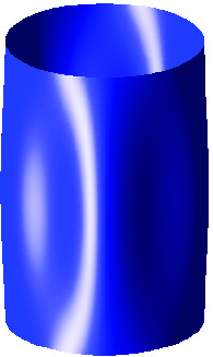
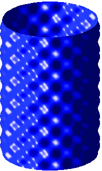
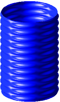
Figure 1: Buckling modes corresponding, left to right, to $m=1$, $m=M(h)/2$ and $m=M(h)$ on the Koiter’s circle.

The figure of the buckling mode corresponding to $m=1$ is shown in Figure 1.

7 Fixed bottom boundary conditions

If the boundary conditions (3.1) are imposed, then we can no longer work with a single Fourier mode space $X(m,n)$, since it has a zero intersection with the space $W_{h}$ defined by (3.4). Hence most of the analysis in Section 6 cannot be done for the fixed bottom boundary conditions. However, we can still compute the buckling load and exhibit buckling modes by modifying the explicit formulas (6.42) for the buckling modes for the boundary conditions (3.2). According to Remark 6.7 the pair $({\mathcal{A}}_{h}\cap W_{h},\mathfrak{K}_{0})$ characterizes buckling for the boundary conditions (3.1). It is therefore clear that

$$\widetilde{\lambda}_{0}(h)=\inf_{\bm{\phi}\in W_{h}\cap{\mathcal{A}}_{h}}\mathfrak{K}_{0}(h,\bm{\phi})\geq\widehat{\lambda}_{0}(h)=\inf_{\bm{\phi}\in{\mathcal{A}}_{h}}\mathfrak{K}_{0}(h,\bm{\phi}).$$

Therefore,

$$\mathop{\underline{\lim}}_{h\to 0}\frac{\widetilde{\lambda}_{0}(h)}{\lambda(h)}\geq 1.$$

If we find a specific test function $\bm{u}_{h}\in W_{h}\cap{\mathcal{A}}_{h}$ such that

$$\lim_{h\to 0}\frac{\mathfrak{K}_{0}(h,\bm{u}_{h})}{\lambda(h)}=1$$

then

$$1=\lim_{h\to 0}\frac{\mathfrak{K}_{0}(h,\bm{u}_{h})}{\lambda(h)}\geq\mathop{\underline{\lim}}_{h\to 0}\frac{\widetilde{\lambda}_{0}(h)}{\lambda(h)}\geq 1.$$

Which proves that $\bm{u}_{h}\in W_{h}$ is a buckling mode and

$$\lim_{h\to 0}\frac{\widetilde{\lambda}_{0}(h)}{\lambda(h)}=1.$$

The idea is to look for the buckling mode in the space $X_{\rm lin}^{0}(n)$ of all functions of the form

$$\begin{cases}u_{r}=\Re\mathfrak{e}(\phi_{r}(z)e^{in\theta}),&\phi_{r}\in W_{0}^{1,2}([0,L];\mathbb{C}),\ \phi_{r}^{\prime}(0)=0,\\ u_{\theta}=\Re\mathfrak{e}(e^{in\theta}(r\phi_{\theta}(z)-(1-r)in\phi_{r}(z))),&\phi_{\theta}\in W_{0}^{1,2}([0,L];\mathbb{C}),\\ u_{z}=\Re\mathfrak{e}((\phi_{z}(z)-(1-r)\phi^{\prime}_{r}(z))e^{in\theta}),&\phi_{z}\in W^{1,2}([0,L];\mathbb{C}),\ \phi_{z}(0)=0.\end{cases}$$ (7.1)

For any $\bm{u}\in X_{\rm lin}^{0}(n(h))$ we have

$$\mathfrak{K}_{0}(h,\bm{u})=\mu\frac{Q_{0}^{0}(\bm{\phi})+\frac{h^{2}}{12}Q_{1}^{0}(\bm{\phi})}{B_{0}(\bm{\phi})},$$

where

$$Q_{0}^{0}(\bm{\phi})=\int_{0}^{L}\{\Lambda|in\phi_{\theta}+\phi^{\prime}_{z}+\phi_{r}|^{2}+2|in\phi_{\theta}+\phi_{r}|^{2}+2|\phi^{\prime}_{z}|^{2}+|in\phi_{z}+\phi^{\prime}_{\theta}|^{2}\}dz,$$

$$Q_{1}^{0}(\bm{\phi})=\int_{0}^{L}\{\Lambda|\phi^{\prime\prime}_{r}-n^{2}\phi_{r}-in\phi_{\theta}|^{2}+2|n^{2}\phi_{r}+in\phi_{\theta}|^{2}+2|\phi^{\prime\prime}_{r}|^{2}+|\phi^{\prime}_{\theta,}-2in\phi^{\prime}_{r}|^{2}\}dz,$$

$$B_{0}(\bm{\phi})=\int_{0}^{L}|\phi^{\prime}_{r}|^{2}dz.$$

Even though the fixed bottom boundary conditions prevent the problem to be diagonalized in the Fourier space, it is still useful to represent $\bm{\phi}(z)$ in the form of Fourier series

$$\begin{cases}\displaystyle\phi_{r}(z)=\sum_{m=1}^{\infty}\widehat{\phi}_{r}(m)\sin(\widehat{m}z),\\ \displaystyle\phi_{\theta}(z)=\sum_{m=1}^{\infty}\widehat{\phi}_{\theta}(m)\sin(\widehat{m}z),\\ \displaystyle\phi_{z}(z)=\sum_{m=0}^{\infty}\widehat{\phi}_{z}(m)\cos(\widehat{m}z).\end{cases}$$

The boundary condition (3.1) translate via (7.1) into the additional constraints

$$\sum_{m=1}^{\infty}m\widehat{\phi}_{r}(m)=0,\qquad\sum_{m=0}^{\infty}\widehat{\phi}_{z}(m)=0.$$ (7.2)

In terms of Fourier coefficients we have

$$Q_{0}^{0}(\bm{\phi})=\sum_{m=0}^{\infty}Q_{m}^{0}(\widehat{\bm{\phi}}),\quad Q_{1}^{0}(\bm{\phi})=\sum_{m=1}^{\infty}Q_{m}^{1}(\widehat{\bm{\phi}}),\quad B_{0}(\bm{\phi})=\sum_{m=1}^{\infty}B_{m}^{0}(\widehat{\bm{\phi}}),$$

where

$$Q_{m}^{0}(\widehat{\bm{\phi}})=\Lambda|in\widehat{\phi}_{\theta}-\widehat{m}\widehat{\phi}_{z}+\widehat{\phi}_{r}|^{2}+2|in\widehat{\phi}_{\theta}+\widehat{\phi}_{r}|^{2}+2\widehat{m}^{2}|\widehat{\phi}_{z}|^{2}+|in\widehat{\phi}_{z}+\widehat{m}\widehat{\phi}_{\theta}|^{2},$$

$$Q_{m}^{1}(\widehat{\bm{\phi}})=\Lambda|\widehat{m}^{2}\widehat{\phi}_{r}+n^{2}\widehat{\phi}_{r}+in\widehat{\phi}_{\theta}|^{2}+2|n^{2}\widehat{\phi}_{r}+in\widehat{\phi}_{\theta}|^{2}+2\widehat{m}^{4}|\widehat{\phi}_{r}|^{2}+\widehat{m}^{2}|\widehat{\phi}_{\theta,}-2in\widehat{\phi}_{r}|^{2}.$$

$$B_{m}^{0}(\widehat{\bm{\phi}})=\widehat{m}^{2}|\widehat{\phi}_{r}|^{2}.$$

The fixed bottom boundary conditions do not place any additional constraints on the Fourier coefficients of $\phi_{\theta}$. Therefore, we can minimize $Q_{m}^{0}+h^{2}Q_{m}^{1}/12$ in $\widehat{\phi}_{\theta}$ to obtain an explicit expression of $\widehat{\phi}_{\theta}(m)$ in terms of $\widehat{\phi}_{r}(m)$ and $\widehat{\phi}_{z}(m)$. However, we may simplify the algebra by recalling that the functional $\mathfrak{K}^{*}$ could be used to compute the buckling load. We therefore determine the relation between $\widehat{\phi}_{\theta}(m)$ and $\widehat{\phi}_{r}(m)$, and $\widehat{\phi}_{z}(m)$ by minimizing $Q_{m}^{0}$ in $\widehat{\phi}_{\theta}$. We obtain

$$\widehat{\phi}_{\theta}=in\frac{(\Lambda+2)\widehat{\phi}_{r}-(\Lambda+1)\widehat{m}\widehat{\phi}_{z}}{(\Lambda+2)n^{2}+\widehat{m}^{2}}.$$ (7.3)

We now cook-up a test function based on (6.42).

Let $m=m(h)$ be such that

$$\lim_{h\to 0}m(h)=\infty,\qquad\lim_{h\to 0}m(h)\sqrt{h}=0.$$ (7.4)

Let $n=n(h)=n(m(h))$ be given by (6.45). We remark that under our assumptions $n(h)\gg m(h)$. Let

$$\phi_{r}=\left(\frac{\sin(\widehat{m}z)}{\widehat{m}}-\frac{\sin(\widehat{m+2}z)}{\widehat{m+1}}\right)\cos(n\theta).$$

This function satisfies all the required boundary conditions in (7.1). It’s $z$-derivative also vanishes at the top of the cylinder, even though we do not require it. If we define $\widehat{\phi}_{z}(m)$ by (6.42) then the resulting function $\phi_{z}$ will not vanish exactly at the bottom of the cylindrical shell. That is why we modify (6.42) as follows

$$\phi_{z}=T(m,n)(\cos(\widehat{m+2}z)-\cos(\widehat{m}z))\cos(n\theta),$$ (7.5)

where

$$T(m,n)=\frac{(\Lambda+2)n^{2}-\Lambda\widehat{m}^{2}}{(\Lambda+2)(n^{2}+\widehat{m}^{2})^{2}}.$$

Once again we observe that $\phi_{z}$ vanishes not only at the bottom boundary, but also at the top, accommodating even pure displacement boundary conditions on top and bottom edges. We may simplify our test function if we retain only the necessary asymptotics as $h\to 0$ in (7.3) and (7.5):

$$\begin{cases}\phi_{r}=\left(\dfrac{\sin(\widehat{m}z)}{\widehat{m}}-\dfrac{\sin(\widehat{m+2}z)}{\widehat{m+2}}\right)\cos(n\theta),\\ \phi_{z}=\displaystyle\frac{1}{n^{2}}(\cos(\widehat{m+2}z)-\cos(\widehat{m}z))\cos(n\theta),\\ \phi_{\theta}=-\displaystyle\frac{1}{n}(\gamma(m,n)\sin(\widehat{m}z)-\gamma(m+2,n)\sin(\widehat{m+2}z))\sin(n\theta),\end{cases}$$ (7.6)

$$\gamma(m,n)=\displaystyle\frac{1}{\widehat{m}}+\frac{\Lambda\widehat{m}}{(\Lambda+2)n^{2}}.$$

Substituting this into $\mathfrak{K}_{0}$ we obtain

$$\lim_{h\to 0}\frac{\mathfrak{K}_{0}(h,\bm{\phi})}{h}=\lim_{h\to 0}\frac{\mu}{2}\sqrt{\frac{\Lambda+1}{3}}\left(2+\frac{(\widehat{m+2})^{2}}{\widehat{m}^{2}}+\frac{\widehat{m}^{2}}{(\widehat{m+2})^{2}}\right).$$

We conclude that

$$\lim_{h\to 0}\frac{\mathfrak{K}_{0}(h,\bm{\phi})}{h}=\lim_{h\to 0}\frac{\lambda(h)}{h}=2\mu\sqrt{\frac{\Lambda+1}{3}},$$

since

$$\lim_{h\to 0}\frac{(\widehat{m+2})^{2}}{\widehat{m}^{2}}=1.$$

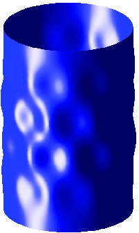
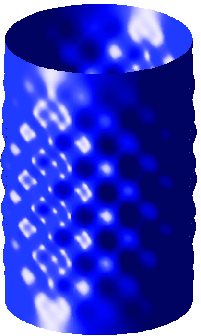
Figure 2: Buckling mode (7.1), (7.6) corresponding, left to right, to $m(h)\sim h^{-1/8}$, $h^{-1/4}$ and $h^{-3/8}$.

Thus, the test functions (7.6) are buckling modes for any $m(h)$ satisfying (7.4). Figure 2 shows the buckling mode (7.6) for

$$\widehat{m(h)}=\left(\frac{4\sqrt{3(\Lambda+1)}}{h(\Lambda+2)}\right)^{\alpha},\quad\alpha=1/8,\ 1/4,3/8.$$

8 Discussion

The key observation in our analysis is that for the test functions $\bm{U}^{h}$ (3.9) we have

$$\mathfrak{S}_{h}(\bm{U}^{h})=O(\|e(\bm{U}^{h})\|^{2})=O(K(V_{h})\|\nabla\bm{U}^{h}\|^{2}).$$

However, the asymptotics of the destabilizing compressiveness term

$$\mathfrak{C}_{h}(\bm{U}^{h})=\int_{\Omega_{h}}(\bm{\sigma}_{h},(\nabla\bm{U}^{h})^{T}\nabla\bm{U}^{h})d\bm{x}$$

depends strongly on the structure of the tensor

$$\bm{\sigma}^{0}(\theta,z)=\lim_{h\to 0}\bm{\sigma}_{h}(r,\theta,z),$$

We saw that for the perfect cylinder $\bm{\sigma}^{0}=\bm{\sigma}_{h}$ is given by (5.4) and hence

$$\mathfrak{C}_{h}(\bm{U}^{h})=O\left(\frac{\|e(\bm{U}^{h})\|^{2}}{h}\right),$$

If we assume that

$$\bm{\sigma}_{h}(r,\theta,z;h)=\bm{\sigma}^{0}(\theta,z)+h\bm{\tau}(\theta,z)+(r-1)\bm{\sigma}^{1}(\theta,z)+O(h^{2}).$$ (8.7)

Substituting it into the equilibrium equation $\nabla\cdot\bm{\sigma}^{h}=\bm{0}$ and passing to the limit as $h\to 0$, we obtain

$$\begin{cases}\sigma^{1}_{rr}+\sigma^{0}_{r\theta,\theta}+\sigma^{0}_{rr}-\sigma^{0}_{\theta\theta}+\sigma^{0}_{rz,z}=0,\\ \sigma^{1}_{r\theta}+\sigma^{0}_{\theta\theta,\theta}+2\sigma^{0}_{r\theta}+\sigma^{0}_{\theta z,z}=0,\\ \sigma^{1}_{rz}+\sigma^{0}_{\theta z,\theta}+\sigma^{0}_{rz}+\sigma^{0}_{zz,z}=0.\end{cases}$$ (8.8)

The traction-free boundary conditionon the lateral boundary of the shell $r=1\pm h/2$ implies that

$$\bm{\sigma}^{0}(\theta,z)\bm{e}_{r}=\bm{\sigma}^{1}(\theta,z)\bm{e}_{r}=\bm{\tau}(\theta,z)\bm{e}_{r}=\bm{0}$$

for all $(\theta,z)\in\mathbb{T}\times(0,L)$. Substituting these equations into (8.8) we obtain

$$\sigma_{rr}^{0}=0,\quad\sigma_{r\theta}^{0}=0,\quad\sigma_{rz}^{0}=0,\quad\sigma^{0}_{\theta\theta}=0.$$

We also obtain $\sigma^{0}_{\theta z,z}=0$ and $\sigma^{0}_{\theta z,\theta}+\sigma^{0}_{zz,z}=0$. Solving these equations results in the following form for $\bm{\sigma}^{0}$:

$$\bm{\sigma}^{0}(\theta,z)=\left[\begin{array}[]{ccc}0&0&0\\ 0&0&s(\theta)\\ 0&s(\theta)&t(\theta)-zs^{\prime}(\theta)\end{array}\right].$$ (8.9)

for some functions $s(\theta)$ and $t(\theta)$. For generic choices of $s(\theta)$ and $t(\theta)$ we obtain

$$\mathfrak{C}_{h}(\bm{U}^{h})=O\left(\frac{\|e(\bm{U}^{h})\|^{2}}{h^{5/4}}\right),$$

resulting in $\lambda(h)=O(h^{5/4})$. One might conjecture that the imperfections of load can produce a non-homogeneous trivial branch leading to $\bm{\sigma}^{0}$ given by (8.9) and hence to the dramatic change in the asymptotic behavior of $\lambda(h)$.

If we disregard the calculations leading to (8.9) and assume for a moment that $\sigma^{0}_{\theta\theta}\not=0$ then

$$\mathfrak{C}_{h}(\bm{U}^{h})=O\left(\frac{\|e(\bm{U}^{h})\|^{2}}{h^{3/2}}\right)=O\left(\frac{\|e(\bm{U}^{h})\|^{2}}{K(V_{h})}\right).$$

It may be conjectured that imperfection of shape can be mathematically described by such tensor $\bm{\sigma}^{0}$. In this case the critical load has the asymptotics $\lambda(h)\sim K(V_{h})=O(h^{3/2})$. We note that the exponents $5/4=1.25$ and $3/2=1.5$ are close the upper and lower limits of experimentally determined behavior of the buckling load [2, 8].

Observe that $\mathfrak{C}_{h}(\bm{\phi})$ cannot be larger than $\|e(\bm{\phi})\|^{2}/K(V_{h})$. Therefore, if the predicted buckling load $\lambda(h)\sim K(V_{h})$ (Euler buckling in the terminology of [6]) then the imperfections of load and shape will have negligible effect on the buckling load as in the case of straight solid struts and flat plates.

Acknowledgments. We are grateful to Lev Truskinovsky for reading the entire manuscript and suggesting many improvements in the exposition. This material is based upon work supported by the National Science Foundation under Grants No. 1008092.

Appendix A Proof of Theorem 3.1

The proof of Theorem 3.1 is quite involved and will be split into several relatively simple steps.

A.1 Zero boundary conditionon a rectangle

For any vector field $\bm{U}=(u,v)$ on $\Omega=[0,h]\times[0,L]$ and any $\alpha\in[-1,1]$ we define

$$\bm{G}_{\alpha}=\left[\begin{array}[]{cc}\displaystyle{u_{x}}&\displaystyle{u_{y}}\\[4.30554pt] \displaystyle{v_{x}}&\displaystyle{v_{y}+\alpha u}\end{array}\right],\qquad\bm{e}_{\alpha}=\displaystyle\frac{1}{2}(\bm{G}_{\alpha}+\bm{G}_{\alpha}^{T})=\left[\begin{array}[]{cc}\displaystyle{u_{x}}&\displaystyle{\displaystyle\frac{1}{2}(u_{y}+v_{x})}\\[4.30554pt] \displaystyle{\displaystyle\frac{1}{2}(u_{y}+v_{x})}&\displaystyle{v_{y}+\alpha u}\end{array}\right].$$

Theorem A.1.

Suppose that the vector field $\bm{U}=(u,v)\in C^{1}(\overline{\Omega};\mathbb{R}^{2})$ satisfies $u(x,0)=u(x,L)=\bm{0}$. Then for any $\alpha\in[-1,1]$, any $h\in(0,1)$ and any $L>0$

$$\|\bm{G}_{\alpha}\|^{2}\leq 100\|\bm{e}_{\alpha}\|\left(\frac{\|u\|}{h}+\|\bm{e}_{\alpha}\|\right).$$

We emphasize that there are no boundary conditions imposed on $v(x,y)$.

Proof.

First we prove several auxiliary lemmas.

Lemma A.2.

Suppose $w(x,y)$ is harmonic in $[0,h]\times[0,L]$, and satisfies $w(x,0)=w(x,L)=0$. Then

$$\|w_{y}\|^{2}\leq\frac{2\sqrt{3}}{h}\|w\|\|w_{x}\|+\|w_{x}\|^{2}.$$ (A.1)

Proof.

If $w(x,y)$ is harmonic and satisfies $w(x,0)=w(x,L)=0$ then it must have the expansion

$$w(x,y)=\sum_{n=1}^{\infty}(A_{n}e^{\frac{\pi nx}{L}}+B_{n}e^{-\frac{\pi nx}{L}})\sin\left(\frac{\pi ny}{L}\right).$$

Therefore,

$$\|w\|^{2}=\frac{Lh}{2}\sum_{n=1}^{\infty}\left\{\psi\left(\frac{\pi nh}{L}\right)\left(A_{n}^{2}e^{\frac{\pi nh}{L}}+B_{n}^{2}e^{\frac{-\pi nh}{L}}\right)+2A_{n}B_{n}\right\},\qquad\psi(x)=\frac{\sinh(x)}{x}.$$

In the expansion of $w_{y}$ we simply multiply $A_{n}$ and $B_{n}$ by $\pi n/L$, while in the expansion of $w_{x}$ we multiply $A_{n}$ by $\pi n/L$ and $B_{n}$ by $-\pi n/L$:

$$\|w_{y}\|^{2}=\frac{Lh}{2}\sum_{n=1}^{\infty}\frac{\pi^{2}n^{2}}{L^{2}}\left\{\psi\left(\frac{\pi nh}{L}\right)\left(A_{n}^{2}e^{\frac{\pi nh}{L}}+B_{n}^{2}e^{\frac{-\pi nh}{L}}\right)+2A_{n}B_{n}\right\},$$

$$\|w_{x}\|^{2}=\frac{Lh}{2}\sum_{n=1}^{\infty}\frac{\pi^{2}n^{2}}{L^{2}}\left\{\psi\left(\frac{\pi nh}{L}\right)\left(A_{n}^{2}e^{\frac{\pi nh}{L}}+B_{n}^{2}e^{\frac{-\pi nh}{L}}\right)-2A_{n}B_{n}\right\},$$

The numbers $A_{n}$ and $B_{n}$ can be arbitrary, but such that all the series converge. We can therefore change variables

$$a_{n}=A_{n}e^{\frac{\pi nh}{2L}},\qquad b_{n}=B_{n}e^{-\frac{\pi nh}{2L}},\qquad\tau_{n}=\frac{\pi nh}{L}$$

Then

$$\frac{\|w\|^{2}}{h^{2}}=\frac{Lh}{2}\sum_{n=1}^{\infty}\frac{\pi^{2}n^{2}}{\tau_{n}^{2}L^{2}}\{(\psi(\tau_{n})-1)(a_{n}^{2}+b_{n}^{2})+(a_{n}+b_{n})^{2}\},$$

$$\|w_{y}\|^{2}=\frac{Lh}{2}\sum_{n=1}^{\infty}\frac{\pi^{2}n^{2}}{L^{2}}\{(\psi(\tau_{n})-1)(a_{n}^{2}+b_{n}^{2})+(a_{n}+b_{n})^{2}\},$$

$$\|w_{x}\|^{2}=\frac{Lh}{2}\sum_{n=1}^{\infty}\frac{\pi^{2}n^{2}}{L^{2}}\{(\psi(\tau_{n})-1)(a_{n}^{2}+b_{n}^{2})+(a_{n}-b_{n})^{2}\},$$

Obviously,

$$\|w_{y}\|^{2}-\|w_{x}\|^{2}=2Lh\sum_{n=1}^{\infty}\frac{\pi^{2}n^{2}}{L^{2}}a_{n}b_{n}\leq 2Lh\sum_{n\in{\mathcal{P}}}\frac{\pi^{2}n^{2}}{L^{2}}a_{n}b_{n},\qquad{\mathcal{P}}=\{n\in\mathbb{N}:a_{n}b_{n}>0.\}.$$

Next we estimate

$$\frac{\|w\|^{2}}{h^{2}}\geq\frac{Lh}{2}\sum_{n\in{\mathcal{P}}}\frac{\pi^{2}n^{2}}{\tau_{n}^{2}L^{2}}\{(\psi(\tau_{n})-1)(a_{n}^{2}+b_{n}^{2})+(a_{n}+b_{n})^{2}\}\geq Lh\sum_{n\in{\mathcal{P}}}\frac{\pi^{2}n^{2}}{\tau_{n}^{2}L^{2}}(\psi(\tau_{n})+1)a_{n}b_{n}.$$

Similarly,

$$\|w_{x}\|^{2}\geq Lh\sum_{n\in{\mathcal{P}}}\frac{\pi^{2}n^{2}}{L^{2}}(\psi(\tau_{n})-1)a_{n}b_{n}.$$

Now we have

$$\sum_{n\in{\mathcal{P}}}\frac{\pi^{2}n^{2}}{L^{2}}a_{n}b_{n}=\sum_{n\in{\mathcal{P}}}\left(\frac{\pi n}{L}\sqrt{(\psi(\tau_{n})-1)a_{n}b_{n}}\right)\left(\frac{\pi n}{L}\sqrt{\frac{a_{n}b_{n}}{\psi(\tau_{n})-1}}\right).$$

Applying the Cauchy-Schwartz inequality we obtain

$$\sum_{n\in{\mathcal{P}}}\frac{\pi^{2}n^{2}}{L^{2}}a_{n}b_{n}\leq\sqrt{\sum_{n\in{\mathcal{P}}}\frac{\pi^{2}n^{2}}{L^{2}}(\psi(\tau_{n})-1)a_{n}b_{n}}\sqrt{\sum_{n\in{\mathcal{P}}}\Phi(\tau_{n})\frac{\pi^{2}n^{2}}{\tau_{n}^{2}L^{2}}(\psi(\tau_{n})+1)a_{n}b_{n}},$$

where

$$\Phi(\tau)=\frac{\tau^{2}}{\psi(\tau)^{2}-1}=\frac{\tau^{4}}{\sinh^{2}(\tau)-\tau^{2}}.$$

The function $\Phi(\tau)$ is monotone decreasing on $(0,+\infty)$, and hence, $\Phi(\tau_{n})\leq\Phi(\tau_{1})\leq\Phi(0)=3$. Therefore,

$$\|w_{y}\|^{2}-\|w_{x}\|^{2}\leq\frac{2\sqrt{\Phi(\pi h/L)}}{h}\|w\|\|w_{x}\|,$$ (A.2)

and the inequality (A.1) follows. The inequality (A.2) is sharp, since it turns into equality for

$$w(x,y)=\cosh\left(\frac{\pi}{L}\left(x-\frac{h}{2}\right)\right)\sin\left(\frac{\pi y}{L}\right).$$

∎

Suppose $w(x,y)$ solves

$$\begin{cases}\Delta w(x,y)=0,&(x,y)\in\Omega\\ w(x,y)=u(x,y),&(x,y)\in\partial\Omega,\end{cases}$$ (A.3)

where $\Omega=[0,h]\times[0,L]$. Then $\nabla w$ is the Helmholtz projection of $\nabla u$ onto the space of the divergence-free fields in $L^{2}(\Omega;\mathbb{R}^{2})$.

Lemma A.3.

Suppose that the vector field $\bm{U}=(u,v)\in C^{1}(\overline{\Omega};\mathbb{R}^{2})$ satisfies $\bm{U}(x,0)=\bm{U}(x,L)=\bm{0}$. Let $w(x,y)$ be defined by (A.3). Then for any $\alpha\in[-1,1]$, any $h\in(0,1)$ and any $L>0$

$$\|\nabla u-\nabla w\|\leq\left(\sqrt{2}+\displaystyle\frac{1}{\pi}\right)\|\bm{e}_{\alpha}\|,\qquad\|u-w\|\leq\frac{h}{\pi}\left(\sqrt{2}+\displaystyle\frac{1}{\pi}\right)\|\bm{e}_{\alpha}\|.$$ (A.4)

Proof.

This follows your note with tighter constants.

$$\Delta(u-w)=\Delta u=(e_{11}-e_{22})_{x}+2(e_{12})_{y}+\alpha e_{11}.$$

Multiplying by $u-w$ and integrating we get

$$\|\nabla(u-w)\|^{2}=\int_{\Omega}\{(e_{11}-e_{22})(u-w)_{x}+2e_{12}(u-w)_{y}+\alpha e_{11}(w-u)\}d\bm{x}$$

By Cauchy-Schwartz inequality we get

$$\|\nabla(u-w)\|^{2}\leq\|\bm{e}_{\alpha}\|(\sqrt{2}\|\nabla(u-w)\|+|\alpha|\|u-w\|).$$

By Poincaré

$$\int_{0}^{h}|u-w|^{2}dx\leq\frac{h^{2}}{\pi^{2}}\int_{0}^{h}|(u-w)_{y}|^{2}dx.$$

Hence,

$$\|u-w\|\leq\frac{h}{\pi}\|\nabla(u-w)\|,$$

and (A.4) follows. ∎

We are now ready to prove the theorem. For simplicity of notation we denote

$$K_{0}=\frac{1}{\pi}\left(\sqrt{2}+\displaystyle\frac{1}{\pi}\right).$$

By the triangle inequality and Lemma A.3 we get

$$\|\bm{G}_{\alpha}\|^{2}=\|\bm{e}_{\alpha}\|^{2}+\displaystyle\frac{1}{2}\|v_{x}-u_{y}\|^{2}=\|\bm{e}_{\alpha}\|^{2}+\displaystyle\frac{1}{2}\|(v_{x}+u_{y})-2(u_{y}-w_{y})-2w_{y}\|^{2}\leq\\ \|\bm{e}_{\alpha}\|^{2}+\frac{3}{2}\|u_{y}+v_{x}\|^{2}+6\|u_{y}-w_{y}\|^{2}+6\|w_{y}\|^{2}\leq(4+6\pi^{2}K_{0}^{2})\|\bm{e}_{\alpha}\|^{2}+6\|w_{y}\|^{2}.$$

To estimate $\|w_{y}\|$ via Lemma A.2 we have by the triangle inequality and Lemma A.3

$$\|w\|\leq\|u\|+\|u-w\|\leq\|u\|+K_{0}h\|\bm{e}_{\alpha}\|,$$

$$\|w_{x}\|\leq\|u_{x}\|+\|w_{x}-u_{x}\|\leq(1+\pi K_{0})\|\bm{e}_{\alpha}\|.$$

Therefore,

$$\|w_{y}\|^{2}\leq\frac{2\sqrt{3}(1+\pi K_{0})}{h}\|u\|\|\bm{e}_{\alpha}\|+(1+\pi K_{0})(1+(2\sqrt{3}+\pi)K_{0})\|\bm{e}_{\alpha}\|^{2}.$$

Thus,

$$\|\bm{G}_{\alpha}\|^{2}\leq\frac{12\sqrt{3}(1+\pi K_{0})}{h}\|u\|\|\bm{e}_{\alpha}\|+K_{1}\|e_{\alpha}\|^{2},$$

where

$$K_{1}=4+6\pi^{2}K_{0}^{2}+6(1+\pi K_{0})(1+(2\sqrt{3}+\pi)K_{0}).$$

Rounding the constants up to the next integer we obtain

$$\|\bm{G}_{\alpha}\|^{2}\leq 99\|\bm{e}_{\alpha}\|^{2}+\frac{57}{h}\|u\|\|\bm{e}_{\alpha}\|.$$

The theorem is proved now. ∎

A.2 Periodic boundary conditions on a rectangle

Theorem A.4.

Suppose that the vector field $\bm{U}=(u,v)\in C^{1}([0,h]\times[0,2\pi];\mathbb{R}^{2})$ satisfies $u(x,0)=u(x,2\pi)$. Then there exists an absolute numerical constant $C_{0}>0$ such that for any $\alpha\in[-1,1]$ and any $h\in(0,1)$

$$\|\bm{G}_{\alpha}\|^{2}\leq C_{0}\|\bm{e}_{\alpha}\|\left(\frac{\|u\|}{h}+\|\bm{e}_{\alpha}\|\right).$$

Proof.

For any fixed $t\in[0,2\pi]$ denote $\bm{U}_{t}=(u-u(x,t),v+\alpha yu(x,t))$ and $\Omega_{t}=[0,h]\times[t,t+2\pi].$ Observe that $\bm{U}_{t}$ satisfies zero boundary conditions on the horizontal boundary of $\Omega_{t}.$ We apply now Theorem  A.1 to the displacement $\bm{U}_{t}$ in $\Omega_{t},$

$$\|\bm{G}_{\alpha}(\bm{U}_{t})\|^{2}\leq\frac{100}{h}\|e(\bm{G}_{\alpha}(\bm{U}_{t}))\|\cdot\|u_{t}\|+100\|e(\bm{G}_{\alpha}(\bm{U}_{t}))\|^{2}.$$ (A.5)

Note that

$$\bm{G}_{\alpha}(\bm{U}_{t})=\begin{bmatrix}u_{x}-u_{x}(x,t)&u_{y}\\ v_{x}+\alpha yu_{x}(x,t)&v_{y}+u\\ \end{bmatrix}=\bm{G}_{\alpha}+\begin{bmatrix}-u_{x}(x,t)&0\\ \alpha yu_{x}(x,t)&0\\ \end{bmatrix}$$

and

$$e(\bm{G}_{\alpha}(\bm{U}_{t}))=\begin{bmatrix}u_{x}-u_{x}(x,t)&\frac{1}{2}(u_{y}+v_{x}+\alpha yu_{x}(x,t))\\ \frac{1}{2}(u_{y}+v_{x}+\alpha yu_{x}(x,t))&v_{y}+u\\ \end{bmatrix}=$$

$$=\bm{e}_{\alpha}+\begin{bmatrix}-u_{x}(x,t)&\frac{1}{2}\alpha yu_{x}(x,t)\\ \frac{1}{2}\alpha yu_{x}(x,t)&0\\ \end{bmatrix},$$

thus

$$\|\bm{G}_{\alpha}\|\leq\|\bm{G}_{\alpha}(\bm{U}_{t})\|+(1+2\pi)\|u_{x}(x,t)\|,$$

$$\|e(\bm{G}_{\alpha}(\bm{U}_{t}))\|\leq\|\bm{e}_{\alpha}\|+(1+2\pi)\|u_{x}(x,t)\|$$

and

$$\|u_{t}\|\leq\|u\|+\|u(x,t)\|.$$

Utilizing now (A.5) and taking into account the last three inequalities we arrive at

$$\|\bm{G}_{\alpha}\|^{2}\leq 2\|\bm{G}_{\alpha}(\bm{U}_{t})\|^{2}+2(1+2\pi)^{2}\|u_{x}(x,t)\|^{2}\leq$$

$$\leq\frac{200}{h}\|e(\bm{G}_{\alpha}(\bm{U}_{t}))\|\cdot\|u_{t}\|+200\|e(\bm{G}_{\alpha}(\bm{U}_{t}))\|^{2}+2(1+2\pi)^{2}\|u_{x}(x,t)\|^{2}\leq$$

$$\leq\frac{200}{h}\big{(}\|\bm{e}_{\alpha}\|+(1+2\pi)\|u_{x}(x,t)\|\big{)}\big{(}\|u\|+\|u(x,t)\|\big{)}+$$

$$+200\big{(}\|\bm{e}_{\alpha}\|+(1+2\pi)\|u_{x}(x,t)\|\big{)}^{2}+2(1+2\pi)^{2}\|u_{x}(x,t)\|^{2}$$ (A.6)

We complete the proof integrating (A.6) in $t$ over $[0,L]$ and then estimating each summand applying the Schwartz inequality as follows

$$\int_{0}^{L}\|u_{x}(x,t)\|\,\mathrm{d}t\leq\Big{(}L\int_{0}^{L}\|u_{x}(x,t)\|^{2}\,\mathrm{d}t\Big{)}^{\frac{1}{2}}=$$

$$=\Big{(}L^{2}\int_{0}^{L}\int_{0}^{h}u_{x}^{2}(x,t)\,\mathrm{d}x\,\mathrm{d}t\Big{)}^{\frac{1}{2}}=L\|u_{x}\|\leq L\|\bm{e}_{\alpha}\|,$$

similarly

$$\int_{0}^{L}\|u(x,t)\|\,\mathrm{d}t\leq L\|u\|,$$

$$\int_{0}^{L}\|u_{x}(x,t)\|^{2}\,\mathrm{d}t=L\|u_{x}\|^{2}\leq L\|\bm{e}_{\alpha}\|^{2},$$

$$\int_{0}^{L}\|u_{x}(x,t)\|\|u(x,t)\|\,\mathrm{d}t\leq\Big{(}\int_{0}^{L}\|u_{x}(x,t)\|^{2}\,\mathrm{d}t\cdot\int_{0}^{L}\|u(x,t)\|^{2}\,\mathrm{d}t\Big{)}^{\frac{1}{2}}=$$

$$=L\|u_{x}\|\|u\|\leq L\|\bm{e}_{\alpha}\|\|u\|.$$

∎

Let

$$\bm{G}_{*}=\left[\begin{array}[]{cc}\displaystyle{u_{x}}&\displaystyle{u_{y}-v}\\[4.30554pt] \displaystyle{v_{x}}&\displaystyle{v_{y}+u}\end{array}\right],\qquad\bm{e}_{*}=\displaystyle\frac{1}{2}(\bm{G}_{*}+\bm{G}_{*}^{T}).$$

Theorem A.5.

Suppose that the vector field $\bm{U}=(u,v)\in C^{1}([0,h]\times[0,2\pi];\mathbb{R}^{2})$ satisfies $\bm{U}(x,0)=\bm{U}(x,2\pi)$. Then there exist absolute numerical constants $\sigma>0$ and $C_{0}>0$ such that for any $h\in(0,\sigma)$

$$\|\bm{G}_{*}\|^{2}\leq C_{0}\left(\|\bm{e}_{*}\|^{2}+\|\bm{e}_{*}\|\frac{\|u\|}{h}+\|v\|^{2}\right).$$

Proof.

Let $\bm{V}=(u,(1-x)v)$, and let

$$\bm{G}_{1}=G_{1}(\bm{V}),\qquad\bm{e}_{1}=\displaystyle\frac{1}{2}(\bm{G}_{1}+\bm{G}_{1}^{T}).$$

We compute

$$\bm{G}_{*}=\bm{G}_{1}+\left[\begin{array}[]{cc}\displaystyle{0}&\displaystyle{-v}\\[4.30554pt] \displaystyle{v+xv_{x}}&\displaystyle{xv_{y}}\end{array}\right],\qquad\bm{e}_{1}=\bm{e}_{*}+\left[\begin{array}[]{cc}\displaystyle{0}&\displaystyle{-\dfrac{x}{2}v_{x}}\\[4.30554pt] \displaystyle{-\dfrac{x}{2}v_{x}}&\displaystyle{-xv_{y}}\end{array}\right].$$

Thus we immediately obtain that

$$\|\bm{G}_{*}\|^{2}\leq 6(\|\bm{G}_{1}\|^{2}+\|v\|^{2}+h^{2}(\|v_{x}\|^{2}+\|v_{y}\|^{2}).$$

and

$$\|\bm{e}_{1}\|\leq\|\bm{e}_{*}\|+h(\|v_{x}\|+\|v_{y}\|)$$ (A.7)

We also estimate

$$\|v_{x}\|\leq\|\bm{G}_{*}\|,\qquad\|v_{y}\|\leq\|v_{y}+u\|+\|u\|\leq\|\bm{e}_{*}\|+\|u\|.$$ (A.8)

Now we apply Theorem A.4 to the vector field $\bm{V}$ and $\alpha=1$, and obtain

$$\|\bm{G}_{*}\|^{2}\leq C_{0}\left(\|\bm{e}_{1}\|^{2}+\|\bm{e}_{1}\|\frac{\|u\|}{h}+\|v\|^{2}+h^{2}(\|v_{x}\|^{2}+\|v_{y}\|^{2})\right).$$

Next we apply (A.7) to the terms containing $\|\bm{e}_{1}\|$ and obtain

$$\|\bm{G}_{*}\|^{2}\leq C_{0}\left(\|\bm{e}_{*}\|^{2}+\|\bm{e}_{*}\|\frac{\|u\|}{h}+\|u\|(\|v_{x}\|+\|v_{y}\|)+\|v\|^{2}+h^{2}(\|v_{x}\|^{2}+\|v_{y}\|^{2})\right).$$

Applying the inequalities (A.8) to the terms containing $\|v_{x}\|$ and $\|v_{y}\|$ we obtain

$$\|\bm{G}_{*}\|^{2}\leq C_{0}\left(\|\bm{e}_{*}\|^{2}+\|\bm{e}_{*}\|\frac{\|u\|}{h}+\|u\|\|\bm{G}_{*}\|+\|u\|^{2}+\|v\|^{2}+h^{2}\|\bm{G}_{*}\|^{2}\right).$$

When $h^{2}<1/(2C_{0})$ we get the inequality

$$\|\bm{G}_{*}\|^{2}\leq C_{0}\left(\|\bm{e}_{*}\|^{2}+\|\bm{e}_{*}\|\frac{\|u\|}{h}+\|u\|\|\bm{G}_{*}\|+\|u\|^{2}+\|v\|^{2}\right).$$

We also have

$$C_{0}\|u\|\|\bm{G}_{*}\|\leq\displaystyle\frac{1}{2}\|\bm{G}_{*}\|^{2}+\frac{C_{0}^{2}}{2}\|u\|^{2}.$$

Thus we obtain

$$\|\bm{G}_{*}\|^{2}\leq C_{0}\left(\|\bm{e}_{*}\|^{2}+\|\bm{e}_{*}\|\frac{\|u\|}{h}+\|u\|^{2}+\|v\|^{2}\right).$$ (A.9)

To finish the proof of the theorem we write $\|u\|^{2}$ using integration by parts and periodic boundary conditions:

$$\|u\|^{2}=(u,u+v_{y})+(u_{y}-v,v)+\|v\|^{2}.$$

Thus,

$$\|u\|^{2}\leq\|u\|\|\bm{e}_{*}\|+\|\bm{G}_{*}\|\|v\|+\|v\|^{2}.$$

Thus, using $2\|u\|\|\bm{e}_{*}\|\leq\|u\|^{2}+\|\bm{e}_{*}\|^{2}$ we obtain

$$\|u\|^{2}\leq\|\bm{e}_{*}\|^{2}+2\|\bm{G}_{*}\|\|v\|+2\|v\|^{2}.$$ (A.10)

Applying this inequality to the $\|u\|^{2}$ term in (A.9) we obtain

$$\|\bm{G}_{*}\|^{2}\leq C_{0}\left(\|\bm{e}_{*}\|^{2}+\|\bm{e}_{*}\|\frac{\|u\|}{h}+\|\bm{G}_{*}\|\|v\|+\|v\|^{2}\right).$$

from which the theorem follows. ∎

A.3 Proof of Lemma 3.2 and the Korn inequality

Step 1. First we prove the analog of Lemma 3.2 in which $\nabla\bm{u}$ and $e(\bm{u})$ are replaced with

$$\bm{A}=\left[\begin{array}[]{ccc}u_{r,r}&u_{r,\theta}-u_{\theta}&u_{r,z}\\ u_{\theta,r}&u_{\theta,\theta}+u_{r}&u_{\theta,z}\\ u_{z,r}&u_{z,\theta}&u_{z,z}\end{array}\right],\qquad e(\bm{A})=\displaystyle\frac{1}{2}(\bm{A}+\bm{A}^{T}).$$

respectively, which is

$$\|\bm{A}\|^{2}\leq C(L)\|e(\bm{A})\|\left(\|e(\bm{A})\|+\frac{\|u_{r}\|}{h}\right).$$ (A.11)

To prove inequality (A.11) we need to estimate three quantities

$$G_{12}^{2}=\|u_{\theta,r}\|^{2}+\|u_{r,\theta}-u_{\theta}\|^{2},\qquad G_{13}^{2}=\|u_{r,z}\|^{2}+\|u_{z,r}\|^{2},\qquad G_{23}^{2}=\|u_{z,\theta}\|^{2}+\|u_{\theta,z}\|^{2}$$

In terms of

$$E_{12}^{2}=\|u_{\theta,r}+u_{r,\theta}-u_{\theta}\|^{2},\qquad E_{13}^{2}=\|u_{r,z}+u_{z,r}\|^{2},\qquad E_{23}^{2}=\|u_{z,\theta}+u_{\theta,z}\|^{2},$$

$$E_{11}^{2}=G_{11}^{2}=\|u_{r,r}\|^{2},\qquad E_{22}^{2}=G_{22}^{2}=\|u_{\theta,\theta}+u_{r}\|^{2},\qquad E_{33}^{2}=G_{33}^{2}=\|u_{z,z}\|^{2}.$$

Step 2. In this step we prove the inequality (3.6) in Lemma 3.2. We start with $G_{23}$. Integration by parts, using the boundary conditions $u_{\theta}=0$ at $z=0$ and $z=L$ and the periodicity in $\theta$ gives

$$|(u_{z,\theta},u_{\theta,z})|=|(u_{z,z},u_{\theta,\theta})|\leq\|u_{z,z}\|\|u_{\theta,\theta}\|\leq E_{33}(E_{22}+\|u_{r}\|).$$

Therefore,

$$G_{23}^{2}=E_{23}^{2}-2(u_{z,\theta},u_{\theta,z})\leq E_{23}^{2}+E_{22}^{2}+E_{33}^{2}+2E_{33}\|u_{r}\|\leq 2\|e(\bm{A})\|(\|e(\bm{A})\|+\|u_{r}\|).$$ (A.12)

Step 3. Next we estimate $G_{13}$. Let us fix $\theta\in[0,2\pi]$ arbitrarily. Next we apply Theorem A.1 to the function

$$\bm{u}(r,z)=(u_{r}(r,\theta,z),u_{z}(r,\theta,z))$$

and $\alpha=0$. We obtain, integrating the inequality over $\theta$ as using the Cauchy-Schwartz for the product term

$$G_{13}^{2}\leq C_{0}\left(E_{11}^{2}+E_{13}^{2}+E_{33}^{2}+\frac{\|u_{r}\|}{h}(E_{11}+E_{13}+E_{33})\right)\leq C_{0}\|e(\bm{A})\|\left(\|e(\bm{A})\|+\frac{\|u_{r}\|}{h}\right),$$ (A.13)

where $C_{0}$ is an absolute numerical constant, independent of $h$ and $L$.

Step 4. Finally we estimate $G_{12}$. Let us fix $z\in[0,L]$ arbitrarily. We apply Theorem A.5 to the function

$$\bm{u}(r,\theta)=(u_{r}(r,\theta,z),u_{\theta}(r,\theta,z))$$

We obtain, integrating the inequality over $z$ and using the Cauchy-Schwartz for the product term

$$G_{12}^{2}\leq C_{0}\left(\|e(\bm{A})\|^{2}+\|e(\bm{A})\|\frac{\|u_{r}\|}{h}+\|u_{\theta}\|^{2}\right)$$

We estimate via the 1D Poincaré inequality

$$\|u_{\theta}\|^{2}\leq\frac{L^{2}}{\pi^{2}}\|u_{\theta,z}\|^{2}\leq\frac{L^{2}}{\pi^{2}}G_{23}^{2}\leq\frac{2L^{2}}{\pi^{2}}(\|e(\bm{A})\|^{2}+\|e(\bm{A})\|\|u_{r}\|).$$ (A.14)

Thus, there exists a constant $C(L)\leq C_{0}(L^{2}(\sigma+1)+1)$ such that

$$G_{12}^{2}\leq C(L)\|e(\bm{A})\|\left(\|e(\bm{A})\|+\frac{\|u_{r}\|}{h}\right).$$

Next we prove the analog of the Korn inequality in which again $\nabla\bm{u}$ and $e(\bm{u})$ are replaced with $\bm{A}$ and $e(\bm{A})$ respectively. Integrating the inequality (A.10) in $z$ and using Cauchy-Schwartz for the product term we obtain

$$\|u_{r}\|^{2}\leq\|e(\bm{A})\|^{2}+2\|\bm{A}\|\|u_{\theta}\|+2\|u_{\theta}\|^{2}\leq\|e(\bm{A})\|^{2}+\epsilon^{2}\|\bm{A}\|^{2}+\left(2+\displaystyle\frac{1}{\epsilon^{2}}\right)\|u_{\theta}\|^{2}$$

for any $\epsilon>0$. The small parameter $\epsilon\in(0,1)$ will be chosen later in an asymptotically optimal way. Applying (A.14) we obtain for sufficiently small $\epsilon$

$$\|u_{r}\|^{2}\leq\left(\frac{L^{2}}{\epsilon^{2}}+1\right)\|e(\bm{A})\|^{2}+\epsilon^{2}\|\bm{A}\|^{2}+\frac{L^{2}}{\epsilon^{2}}\|e(\bm{A})\|\|u_{r}\|.$$

Therefore,

$$\|u_{r}\|^{2}\leq 2\left(\frac{L^{2}}{\epsilon^{2}}+1\right)^{2}\|e(\bm{A})\|^{2}+2\epsilon^{2}\|\bm{A}\|^{2}.$$

Thus,

$$\|u_{r}\|\leq\sqrt{2}\left(\left(\frac{L^{2}}{\epsilon^{2}}+1\right)\|e(\bm{A})\|+\epsilon\|\bm{A}\|\right).$$

Substituting this inequality to (A.11) we conclude that there is a constant $C(L)$, depending only on $L$ such that

$$\|\bm{A}\|^{2}\leq C(L)\left(\displaystyle\frac{1}{h\epsilon^{2}}+\frac{\epsilon^{2}}{h^{2}}\right)\|e(\bm{A})\|^{2}.$$

We now choose $\epsilon=h^{1/4}$ to minimize the bound:

$$\|\bm{A}\|^{2}\leq\frac{C(L)}{h\sqrt{h}}\|e(\bm{A})\|^{2}.$$ (A.15)

Theorem 3.1 is now an immediate consequence of (A.15) and the obvious inequality

$$\|e(\bm{U})-e(\bm{A})\|^{2}\leq\|\nabla\bm{U}-\bm{A}\|^{2}\leq h^{2}\|\bm{A}\|^{2}.$$ (A.16)

Observe that we get from (A.16) and (A.15) that,

$$\|e(\bm{U})-e(\bm{A})\|\leq h\|\bm{A}\|\leq C(L)h^{1/4}\|e(\bm{A})\|.$$ (A.17)

Lemma 3.2 will now follow from (A.16), (A.17) and (A.11).

References

- [1] B. O. Almroth. Postbuckling behaviour of axially compressed circular cylinders. AIAA J, 1:627–633, 1963.
- [2] C. R. Calladine. A shell-buckling paradox resolved. In D. Durban, G. Givoli, and J. G. Simmonds, editors, Advances in the Mechanics of Plates and Shells, pages 119–134. Kluwer Academic Publishers, Dordrecht, 2000.
- [3] G. Friesecke, R. D. James, and S. Müller. A theorem on geometric rigidity and the derivation of nonlinear plate theory from three-dimensional elasticity. Comm. Pure Appl. Math., 55(11):1461–1506, 2002.
- [4] G. Friesecke, R. D. James, and S. Müller. A hierarchy of plate models derived from nonlinear elasticity by gamma-convergence. Arch. Ration. Mech. Anal., 180(2):183–236, 2006.
- [5] D. J. Gorman and R. M. Evan-Iwanowski. An analytical and experimental investigation of the effects of large prebuckling deformations on the buckling of clamped thin-walled circular cylindrical shells subjected to axial loading and internal pressure. Develop. in Theor. and Appl. Mech., 4:415–426, 1970.
- [6] Y. Grabovsky and L. Truskinovsky. The flip side of buckling. Cont. Mech. Thermodyn., 19(3-4):211–243, 2007.
- [7] G. Hunt, G. Lord, and A. Champneys. Homoclinic and heteroclinic orbits underlying the post-buckling of axially-compressed cylindrical shells. Computer methods in applied mechanics and engineering, 170(3):239–251, 1999.
- [8] G. Hunt, G. Lord, and M. Peletier. Cylindrical shell buckling: a characterization of localization and periodicity. DISCRETE AND CONTINUOUS DYNAMICAL SYSTEMS SERIES B, 3(4):505–518, 2003.
- [9] G. Hunt and E. L. Neto. Localized buckling in long axially-loaded cylindrical shells. Journal of the Mechanics and Physics of Solids, 39(7):881 – 894, 1991.
- [10] G. W. Hunt and E. L. Neto. Maxwell critical loads for axially loaded cylindrical shells. Trans. ASME, 60:702–706, 1993.
- [11] W. T. Koiter. On the stability of elastic equilibrium. PhD thesis, Technische Hogeschool (Technological University of Delft), Delft, Holland, 1945.
- [12] M. Lewicka, L. Mahadevan, and M. R. Pakzad. The Föppl-von Kármán equations for plates with incompatible strains. Proc. R. Soc. Lond. Ser. A Math. Phys. Eng. Sci., 467(2126):402–426, 2011. With supplementary data available online.
- [13] M. Lewicka, M. G. Mora, and M. R. Pakzad. The matching property of infinitesimal isometries on elliptic surfaces and elasticity of thin shells. Arch. Ration. Mech. Anal., 200(3):1023–1050, 2011.
- [14] G. Lord, A. Champneys, and G. Hunt. Computation of localized post buckling in long axially compressed cylindrical shells. Philosophical Transactions of the Royal Society of London. Series A: Mathematical, Physical and Engineering Sciences, 355(1732):2137–2150, 1997.
- [15] R. Lorenz. Die nicht achsensymmetrische knickung dünnwandiger hohlzylinder. Physikalische Zeitschrift, 12(7):241–260, 1911.
- [16] M. G. Mora and S. Müller. A nonlinear model for inextensible rods as a low energy -limit of three-dimensional nonlinear elasticity. Ann. Inst. H. Poincaré Anal. Non Linéaire, 21(3):271–293, 2004.
- [17] R. C. Tennyson. An experimental investigation of the buckling of circular cylindrical shells in axial compression using the photoelastic technique. Tech. Report 102, University of Toronto, Toronto, ON, Canada, 1964.
- [18] S. Timoshenko. Towards the question of deformation and stability of cylindrical shell. Vesti Obshestva Tekhnologii, 21:785–792, 1914.
- [19] V. I. Weingarten, E. J. Morgan, and P. Seide. Elastic stability of thin-walled cylindrical and conical shells under axial compression. AIAA J, 3:500–505, 1965.
- [20] N. Yamaki. Elastic Stability of Circular Cylindrical Shells, volume 27 of Appl. Math. Mech. North Holland, 1984.