The Hamiltonian structure and Euler-Poincaré formulation of the Vlasov-Maxwell and gyrokinetic systems

Abstract

We present a new variational principle for the gyrokinetic system, similar to the Maxwell-Vlasov action presented in Ref. Cendra et al., 1998. The variational principle is in the Eulerian frame and based on constrained variations of the phase space fluid velocity and particle distribution function. Using a Legendre transform, we explicitly derive the field theoretic Hamiltonian structure of the system. This is carried out with a modified Dirac theory of constraints, which is used to construct meaningful brackets from those obtained directly from Euler-Poincaré theory. Possible applications of these formulations include continuum geometric integration techniques, large-eddy simulation models and Casimir type stability methods.

I Introduction

An inherent difficulty in studying the dynamics of magnetized plasmas is the enormous separation of important time-scales present in many physical systems of interest. Nonlinear gyrokinetic theory has become an indispensable tool in these inquiries, as it removes the fastest time-scales from the system, while keeping much of important physics relevant to turbulent transportBrizard and Hahm (2007); Krommes (2012); Lin et al. (1998). A particularly nice way to construct a gyrokinetic theory, pioneered in Refs. Dubin et al., 1983; Littlejohn, 1982; Hahm et al., 1988, is to use Lie-transforms to asymptotically change into co-ordinates in which gyro-orbit dynamics are decoupled from the rest of the system. A great advantage of this technique, aside from the entirely systematic and formal procedure, is that the single particle equations are guaranteed to be Hamiltonian, with associated conservation properties. Going further, it is advantageous from both a philosophical and practical standpoint to derive the entire system, including both electromagnetic fields and particles, from a single field-theoretic variational principle. These ideas were explored by SugamaSugama (2000) and BrizardBrizard (2000a), who derived gyrokinetic action principles starting from Maxwell-Vlasov theories, as well as in previous work in Refs. Similon, 1985; Boghosian, 1987; Pfirsch and Morrison, 1985, 1991. Some advantages of this type of formulation are a much simplified derivation of the gyrokinetic Maxwell’s equations and exact energy-momentum conservation laws through Noether’s theorem. Field theories often admit many different variational principles (e.g., for Maxwell-Vlasov see Refs. Pfirsch and Morrison, 1985, 1991; Ye and Morrison, 1992; Brizard, 2000b; Low, 1958; Flå, 1994; Cendra et al., 1998), each with its own advantages and disadvantages. A good example is the difference between Lagrangian and Eulerian actions; the former being constructed in variables that follow particle motion and the latter in variables at fixed points in phase space. It is interesting to explore new types of variational principles, both for the general understanding of the structure of the theory in question, and for practical applications that may require an action of a particular form.

In this work, we present a new gyrokinetic action principle in Eulerian co-ordinates, using Euler-Poincaré reduction theoryHolm et al. (2009, 1998); Newcomb (1962) on the Lagrangian action in Refs. Qin et al., 2007; Sugama, 2000. In addition, using the reduced Legendre transform and a modified version of the Dirac theory of constraints, we derive field theoretic Poisson brackets, similar to the Vlasov-MaxwellMarsden and Weinstein (1982); Morrison (2013); Chandre et al. (2012a); Morrison (1980); Morrison and Greene (1980) and Vlasov-PoissonMorrison (1982); Chandre et al. (2012a) brackets. To our knowledge this is the first explicit demonstration of the field theoretic Hamiltonian structure of the gyrokinetic system (see Refs. Morrison, 2013; Morrison et al., 2012 for a different approach that has recently been used to write down a Poisson brackets for simplified gyrokinetic systems). Our derivation proceeds from the action principle in Ref. Sugama, 2000 and its geometric formulationQin et al. (2007). We do not purport to derive a gyrokinetic co-ordinate system, but rather formulate the theory based on a given single particle Lagrangian. In this way, it is trivial to extend concepts to deal with more complex gyrokinetic theories, for instance theories with self consistent, time-evolving background fieldsQin et al. (2007). We then use the ideas in Ref. Cendra et al., 1998 to reduce the Lagrangian action to one in Eulerian co-ordinates, based on symmetry under the particle-relabeling map from Lagrangian to Eulerian variables. The variations for this new action principle in the Eulerian frame are constrained, and lead to the Euler-Poincaré equations, which are shown to give the standard gyrokinetic Vlasov equation. In some ways the action principle is similar to that of BrizardBrizard (2000a), in that constrained variations must be used, with both theories having a similar form for the variation of the distribution function, $F$. Nevertheless, there are significant differences, particularly that our principle is formulated in terms of the Eulerian phase space fluid velocity and is in standard 6-D phase space, rather than 8-D extended phase space. The Eulerian gyrokinetic action of Refs. Pfirsch and Correa-Restrepo, 2004 is quite different to that presented here, with unconstrained variations in 12-dimensional extended phase space and the use of Hamilton-Jacobi functions in the action functional. For more information on this approach to gyrokientic theory, see Refs. Correa-Restrepo and Pfirsch, 2005a, 2004a, 2004b, b; Pfirsch and Morrison, 1985, 1991. Equipped with the Eulerian action, a reduced Legendre transform is performedCendra et al. (1998), leading straightforwardly to a Poisson bracket. However, this bracket must be reduced to a constraint submanifold before a meaningful form can be obtained, a process that is performed with a modified version of the Dirac theory of constraintsDirac (1950); Chandre et al. (2011, 2010). Finally, we show how to include the electromagnetic fields in the bracket via second application of Dirac theory.

One of our primary motivations in this work is the possibility of utilizing recent ideas from fluid mechanics to develop advanced numerical tools for gyrokinetics. Of particular importance is the idea of geometric integrators, which are designed to numerically conserve various important geometrical properties of the physical system. For instance, having a numerical algorithm that has Hamiltonian structure can be very important, with profound consequences for the long-time conservation propertiesMarsden and West (2001). The theory of finite dimensional geometric integrators is relatively well developedMarsden and West (2001), including an application to single particle guiding center dynamicsQin and Guan (2008); Li et al. (2011); Squire et al. (2012a). However, many aspects of the construction of field-theoretic geometrical integrators are not as well understood, both for practical implementation and the deeper mathematical theory. One approach, which has yielded fruitful results, is to discretize a variational principle and perform variations on the discrete action to derive an integration scheme. Some examples of field theoretic integrators constructed in this way are those for elastomechanicsLew et al. (2003); Marsden et al. (1998), electromagnetismStern et al. (2007), fluids and magnetohydrodynamicsPavlov et al. (2009); Gawlik et al. (2011), and a particle-in-cell (PIC) scheme for the Vlasov-Maxwell systemSquire et al. (2012b). The results presented in this work would be used to construct a continuum Eulerian gyrokinetic integrator, since our variational principle is in Eulerian form. Analogously, a variational principle in Lagrangian form is used to construct a Lagrangian (particle-in-cell) integratorSquire et al. (2012b). We note that in discretizing a variational principle it is obviously not desirable to be in an extended phase space, unless these extra dimensions can somehow be removed after a discretization. As well as integrators, other potential applications of the formulation presented here are the use in stability calculations with Casimir invariants Holm et al. (1985); Kruskal and Oberman (1958) and the construction of regularized models for large-eddy simulationMorel et al. (2011); Graham et al. (2011); Bhat et al. (2005); Holm (2002).

It is significant to note at this point that as the power of modern supercomputing systems continues to advance at a rapid pace toward the exascale ($10^{18}$ floating point operations per second) and beyond, it is quite clear that the associated software development challenges are also increasingly formidable. On the emerging architectures memory and data motion will be serious bottlenecks as the required low-power consumption requirements lead to systems with significant restrictions on available memory and communications bandwidth. Consequently, it will be the case in multiple application domains that it will become necessary to re-visit key algorithms and solvers – with the likelihood that new capabilities will be demanded in order to keep up with the dramatic architectural changes that accompany the impressive increases in compute power. The key challenge here is to develop new methods to effectively utilize such dramatically increased parallel computing power. Algorithms designed using geometric ideas could be very important as simulations of more complex systems are extended to longer times and enlarged spatial domains with high physics fidelity.

The article is organized as follows. In Section II we clarify the differences between Eulerian and Lagrangian action principles for kinetic theories and explain the Euler-Poincaré formulation of the Maxwell-Vlasov systemCendra et al. (1998). This is done with as little reference to the formal mathematics as possible, with the hope that readers unfamiliar with the concepts of Lie groups and algebras will understand the general structure of the theory. Section III explains the construction of the gyrokinetic variational principle, starting from a given single particle gyrokinetic Lagrangian. We give a brief derivation of the Euler-Poincaré equations and show how these lead to a standard form of the gyrokinetic equations. The Hamiltonian structure is dealt with in Section IV. After formally constructing a Poisson bracket from the Lagrangian, we describe how the modified Dirac theory of constraints is used to reduce the bracket to a meaningful form. Finally, numerical applications are briefly discussed in Section V and conclusions given in Section VI.

Throughout this article we use cgs units. In integrals and derivatives, $\bm{z}$ denotes all phase space variables, while $\bm{x}$ denotes just position space variables. Species labels are left out for clarity and implied on the variables $F$ (or $f$), $m$, $e$, $\bm{U}$ and $\bm{M}$, respectively the distribution function, particle mass, particle charge, Eulerian fluid velocity and momenta conjugate to $\bm{U}$. Summation notation is utilized where applicable, with capital indices spanning $1\rightarrow 6$ and lower case indices $1\rightarrow 3$.

II Eulerian and Lagrangian kinetic variational principles

When formulating a variational principle for a continuum fluid-type theory, it is very important to specify whether Lagrangian or Eulerian variables are being used. These notions can be confusing in kinetic plasma theories, since one must consider the motion of the phase-space fluid. In addition, unlike the Euler fluid equations, the equations of motion for kinetic plasma theories have the same form in Eulerian and Lagrangian co-ordinates. Considering the Vlasov-Maxwell system for simplicity, a Lagrangian description gives the equation of motion at the position of a particle carried along by the flow (simply a physical particle). One formulates a variational principle in terms of the fields $\bm{x}\left(\bm{x}_{0},\bm{v}_{0},t\right)$, $\bm{v}\left(\bm{x}_{0},\bm{v}_{0},t\right)$, which are the current position and velocity of an element of phase space that was initially at $\left(\bm{x}_{0},\bm{v}_{0}\right)$. The distribution function is of course just carried along by the Lagrangian co-ordinates, i.e., $f\left(\bm{x}\left(\bm{x}_{0},\bm{v}_{0},t\right),\bm{v}\left(\bm{x}_{0},\bm{v}_{0},t\right)\right)=f_{0}\left(\bm{x}_{0},\bm{v}_{0}\right)$. This type of formulation is the most natural for a kinetic theory, since it is the logical continuum generalization of the action principle for a collection of particles interacting with an electromagnetic field.

An Eulerian variational principle is formulated in terms of the velocity of the phase space fluid at a fixed point, $\bm{U}$, without the notion of where phase space density has been in the past. Thus, at a point $\left(\bm{x},\bm{v}\right)$, the $\bm{x}$ component of the fluid velocity is simply $\bm{v}$ (the co-ordinate), while the $\bm{v}$ component is $\bm{E}+\bm{v}\times\bm{B}/c$. The distribution function $f$, is advected by $\bm{U}$, meaning it is the solution to the differential equation $\partial_{t}f=-\mathcal{L}_{\bm{U}}f=-\bm{U}\cdot\nabla f$, where $\bm{U}$ and $\nabla$ are in six-dimensional phase space. An illustration of these concepts is given in Figure 1 for the 1-D Poisson-Vlasov system (in 2-D phase space). Finally, we note that in discussing the distinction between Eulerian and Lagrangian actions, we refer only to the plasma component of the variational principle; the electromagnetic fields are always in Eulerian co-ordinates.

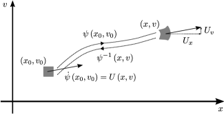
Figure 1: Illustration of the particle relabelling map, $\psi\left(\bm{x}_{0},\bm{v}_{0}\right)$ and its inverse for the one-dimensional Vlasov-Poisson system.

II.1 Euler-Poincaré reduction

This section gives a very informal introduction to Euler-Poincaré theory through a brief review of the Vlasov-Maxwell formulation presented in Ref. Cendra et al., 1998. We purposefully do not use the group theoretical notation of Refs. Holm et al., 2009, 1998; Cendra et al., 1998 (e.g., the $\diamond$ and $\mathrm{ad}^{\star}$ operations) so as to introduce the general ideas to readers not familiar with Lie groups and algebras. Euler-Poincaré type variational principles first appeared in Ref. Newcomb, 1962 in the context of magnetohydrodynamics.

The purpose of the Euler-Poincaré framework is to provide a straightforward method to pass from a Lagrangian to an Eulerian action principle. The important idea is that the Lagrangian is invariant under the right action of the particle relabeling transformation, $\psi\left(\bm{x}_{0},\bm{v}_{0}\right)=\left(\bm{x}\left(\bm{x}_{0},\bm{v}_{0}\right),\bm{v}\left(\bm{x}_{0},\bm{v}_{0}\right)\right)$, which maps plasma particles with initial position $\left(\bm{x}_{0},\bm{v}_{0}\right)$ to their current position $\left(\bm{x},\bm{v}\right)$. In essence, this invariance means that we can eliminate the extraneous particle labeling information and still have an equivalent system. The map $\psi$ acts on $f$ on the right as $f=f_{0}\,\psi^{-1}$, where $f_{0}$ is the initial distribution function. This equation is simply $f\left(\bm{x}\left(\bm{x}_{0},\bm{v}_{0},t\right),\bm{v}\left(\bm{x}_{0},\bm{v}_{0},t\right)\right)=f_{0}\left(\bm{x}_{0},\bm{v}_{0}\right)$, as discussed above. In the electromagnetic part of the Lagrangian $\psi$ does not act on the potentials $\phi$ and $\bm{A}$, since electromagnetic dynamics must be independent of particle labeling. The phase space fluid velocity in the Lagrangian frame is simply $\dot{\psi}\left(\bm{x}_{0},\bm{v}_{0}\right)$, since this is the rate of change of $\left(\bm{x},\bm{v}\right)$ at the position $\left(\bm{x},\bm{v}\right)$. In contrast, the Eulerian phase space fluid velocity is $\dot{\psi}\psi^{-1}$, since this operation first takes $\left(\bm{x},\bm{v}\right)$ back to $\left(\bm{x}_{0},\bm{v}_{0}\right)$ with $\psi^{-1}$ and then gives the velocity at $\left(\bm{x},\bm{v}\right)$ with $\dot{\psi}\left(\bm{x}_{0},\bm{v}_{0}\right)$, see Figure 1.

The starting point for the reduction is a Lagrangian Lagrangian for the Vlasov-Maxwell system. For instance,

$$L =\sum_{s}\int d\bm{x}_{0}d\bm{v}_{0}\,f_{0}\left[\left(\frac{e}{c}\bm{A}\left(\bm{x}\right)+m\bm{v}\right)\cdot\dot{\bm{x}}-\frac{1}{2}m\bm{v}^{2}-e\phi\left(\bm{x}\right)\right]$$

$$+\frac{1}{8\pi}\int d\bm{x}\left[\left|-\nabla\phi-\frac{\partial\bm{A}}{\partial t}\right|^{2}-\left|\nabla\times\bm{A}\right|^{2}\right],$$ (1)

which is very similar to the action principle of LowLow (1958). The Vlasov equation follows from the standard Euler-Lagrange equations for $\psi=\left(\bm{x},\bm{v}\right)$,

$$\frac{d}{dt}\frac{\delta L}{\delta\dot{\psi}}-\frac{\delta L}{\delta\psi}=0,$$ (2)

along with $f\left(\bm{x},\bm{v},t\right)=f_{0}\left(\bm{x}_{0},\bm{v}_{0}\right)$. Maxwell’s equations come from the Euler-Lagrange equations for $\bm{A}$ and $\phi$. This Lagrangian is invariant under the relabeling transformation $\psi$, i.e.,

$$L_{f_{0}}\left(\psi,\dot{\psi},\phi,\dot{\phi},\bm{A},\dot{\bm{A}}\right) =L_{f_{0}\psi^{-1}}\left(\psi\psi^{-1},\dot{\psi}\psi^{-1},\phi,\dot{\phi},\bm{A},\dot{\bm{A}}\right)$$

$$\equiv l\left(\bm{U},\phi,\dot{\phi},\bm{A},\dot{\bm{A}},F\right),$$ (3)

where $\bm{U}=\dot{\psi}\psi^{-1}$ is the Eulerian fluid velocity, a vector field. In recognizing that the distribution function is actually a phase space density, we denote $F=f\,d\bm{x}\wedge d\bm{v}$. Treating $F$ as 6-form rather than a scalar changes the form of certain geometrical operations in the Euler-Poincaré equations [Eqs. (6) and (7)] and is very important for the gyrokinetic Euler-Poincaré treatment (see Section III). Practically speaking, to construct the reduced Lagrangian, $l,$ one simply replaces $\left(\dot{\bm{x}},\dot{\bm{v}}\right)$ with $\bm{U}$, and considers $\bm{x}$ and $\bm{v}$ to be co-ordinates rather than fields. Thus,

$$l =\sum_{s}\int F\left[\left(\frac{e}{c}\bm{A}+m\bm{v}\right)\cdot\bm{U}_{x}-\frac{1}{2}m\bm{v}^{2}-e\phi\left(\bm{x}\right)\right]$$

$$+\frac{1}{8\pi}\int d\bm{x}\left[\left|-\nabla\phi-\frac{\partial\bm{A}}{\partial t}\right|^{2}-\left|\nabla\times\bm{A}\right|^{2}\right],$$ (4)

where $\bm{U}_{x}$ denotes the $\bm{x}$ components of $\bm{U}$. The equations of motion are derived from the reduced Lagrangian $l$, by considering how the unconstrained variations of $\psi$ (used to derive the standard Euler-Lagrange equations) translate into constrained variations of $\bm{U}$ and $F$. This leads to variations of the form

$$\delta\bm{U}=\frac{\partial\eta}{\partial t}-\left[\bm{U},\eta\right],\;\;\delta F=-\mathcal{L}_{\eta}F,$$ (5)

where $\eta$ is in the same space as $\bm{U}$ and vanishes at the endpoints; and $\left[\,,\right]$ is the standard Lie bracket, $\bm{U}.\nabla\eta-\eta.\nabla\bm{U}$. Evolution of $F$ is given by the advection equation

$$\frac{\partial F}{\partial t}+\mathcal{L}_{\bm{U}}F=0,$$ (6)

which arises from the equation $f\left(\bm{x},\bm{v},t\right)=f_{0}\left(\bm{x}_{0},\bm{v}_{0}\right)$. Variation of $\int dt\,l$ with $\delta\bm{U}$ and $\delta F$ leads to the Euler-Poincaré equations,

$$\frac{\partial}{\partial t}\frac{\delta l}{\delta\bm{U}}=-\mathcal{L}_{\bm{U}}\frac{\delta l}{\delta\bm{U}}+F\nabla\frac{\delta l}{\delta F},$$ (7)

where $\delta l/\delta\bm{U}$ is a 1-form density. We give straightforward derivations of Eqs. (5) and (7) in Section III.1 below. Since $F$ is a 6-form, $\mathcal{L}_{\bm{U}}F=\nabla\cdot\left(F\bm{U}\right)$ and Eq. (6) is the conservative form of the Vlasov equation (see Section III.1 for more information). The equations for $\bm{A}$ and $\phi$ are just the standard Euler-Lagrange equations. Calculation of Eq. (7) with the Vlasov-Maxwell reduced Lagrangian [Eq. (4)] leads to

$$\bm{U}_{x}=\bm{v},\>\bm{U}_{v}=\bm{E}+\frac{1}{c}\bm{v}\times\bm{B},$$ (8)

as expected. The fact that there is no need to solve differential equations for components of $\bm{U}$ is related to the strong degeneracy in the system (see Sections III and IV below).

To obtain the Hamiltonian or Lie-Poisson form of the equations, one performs a reduced Legendre transform as,

$$h=\left\langle\bm{M},\bm{U}\right\rangle+\int d\bm{x}\,\bm{A}\cdot\frac{\delta l}{\delta\dot{\bm{A}}}-l,$$ (9)

where $\bm{M}=\delta l/\delta\bm{U}$ and the inner product $\left\langle\,,\right\rangle$ is integration over phase space [see Eq. (37)]. (A thorough treatment of the degeneracies of the system is given in Ref. Cendra et al., 1998.) It is then straightforward to show that

$$\left\{\Gamma,\Theta\right\}_{LP} =-\sum_{s}\int d\bm{z}\bm{M}\cdot\left[\frac{\delta\Gamma}{\delta\bm{M}},\frac{\delta\Theta}{\delta\bm{M}}\right]$$

$$+ \sum_{s}\int d\bm{z}F\left(\frac{\delta\Theta}{\delta\bm{M}}\cdot\nabla\frac{\delta\Gamma}{\delta F}-\frac{\delta\Gamma}{\delta\bm{M}}\cdot\nabla\frac{\delta\Theta}{\delta F}\right)$$

$$- \,4\pi c\int d\bm{x}\left(\frac{\delta\Gamma}{\delta\bm{A}}\cdot\frac{\delta\Theta}{\delta\bm{E}}-\frac{\delta\Theta}{\delta\bm{A}}\cdot\frac{\delta\Gamma}{\delta\bm{E}}\right),$$ (10)

is an infinite dimensional Poisson bracket for the system; that is, $\dot{\bm{M}}=\left\{\bm{M},h\right\}$, $\dot{F}=\left\{F,h\right\}$, $\dot{\bm{E}}=\left\{\bm{E},h\right\}$ and $\dot{\bm{A}}=\left\{\bm{A},h\right\}$ are formally the same as the Euler-Poincaré equations (using the generalized Legendre transform of Ref. Cendra et al., 1998), and the Jacobi identity is satisfied. Nevertheless, this manifestation of the bracket has major problems. In particular, the meaning of functional derivatives with respect to the $\bm{M}$ variables can be unclear, since these are constrained due to the linearity of the Lagrangian in $\bm{U}$. To overcome these problems and formulate a meaningful bracket on the space of plasma densities and electromagnetic fields, we use a modified version of the Dirac theory of constraintsDirac (1950); Pfirsch and Morrison (1991); Morrison et al. (2009). For the convenience of the reader a very brief overview of standard Dirac theory in Appx. A, while the modified version used in parts of this work is covered in Appx. B.

The relevant constraints are

$$\Phi_{i}= M_{i}-F\left(\frac{e}{c}A_{i}+mv_{i}\right)=0,\quad i=1\rightarrow 3,$$

$$\Phi_{j}=M_{j}=0,\quad j=4\rightarrow 6.$$ (11)

We form the constraint matrix $\mathcal{C}_{IJ}\left(\bm{z},\bm{z}^{\prime}\right)=\left\{\Phi_{I}\left(\bm{z}\right),\Phi_{J}\left(\bm{z}^{\prime}\right)\right\}$ and construct the inverse according to the procedure detailed in Appxs. A and B. This comes out to be,

$$\mathcal{C}_{IJ}^{-1} \left(\bm{z},\bm{z}^{\prime}\right)=\frac{1}{mF\left(\bm{z}\right)}\delta\left(\bm{z}-\bm{z}^{\prime}\right)\delta_{ss^{\prime}}$$

$$\times \left(\begin{array}[]{cccccc}0&0&0&1&0&0\\ 0&0&0&0&1&0\\ 0&0&0&0&0&1\\ -1&0&0&0&\frac{e}{mc}B_{z}&-\frac{e}{mc}B_{y}\\ 0&-1&0&-\frac{e}{mc}B_{z}&0&\frac{e}{mc}B_{x}\\ 0&0&-1&\frac{e}{mc}B_{y}&-\frac{e}{mc}B_{x}&0\end{array}\right),$$ (18)

which is simply the single particle Poisson matrix (multiplied by $\delta\left(\bm{z}-\bm{z}^{\prime}\right)/F$) and $\bm{B}$ is a function of $\bm{z}$. We will see a similar connection to the single particle Poisson bracket in the reduction of the gyrokinetic bracket. We then use Eq. (88) and restrict the functionals $\Gamma$ and $\Theta$ to not depend $\bm{M}$, i.e., $\delta\Gamma/\delta\bm{M}=0$ (see Appx. B).

The final result, including a change of variables from $\bm{A}$ to $\bm{B}$, is the Poisson bracket for the Mawell-Vlasov system,

$$\left\{\Gamma,\Theta\right\} =\sum_{s}\frac{1}{m}\int d\bm{z}F\left(\frac{\partial\Gamma_{F}}{\partial\bm{x}}\cdot\frac{\partial\Theta_{F}}{\partial\bm{v}}-\frac{\partial\Theta_{F}}{\partial\bm{x}}\cdot\frac{\partial\Gamma_{F}}{\partial\bm{v}}\right)$$

$$+\sum_{s}\frac{e}{cm^{2}}\int d\bm{z}F\bm{B}\cdot\frac{\partial\Gamma_{F}}{\partial\bm{v}}\times\frac{\partial\Theta_{F}}{\partial\bm{v}}$$

$$+4\pi\sum_{s}\frac{e}{m}\int d\bm{z}\left[\Theta_{F}\frac{\partial}{\partial\bm{v}}\cdot\left(F\frac{\delta\Gamma}{\delta\bm{E}}\right)-\Gamma_{F}\frac{\partial}{\partial\bm{v}}\cdot\left(F\frac{\delta\Theta}{\delta\bm{E}}\right)\right]$$

$$+4\pi c\int d\bm{x}\left(\frac{\partial\Gamma}{\partial\bm{E}}\cdot\nabla\times\frac{\delta\Theta}{\delta\bm{B}}-\frac{\partial\Theta}{\partial\bm{E}}\cdot\nabla\times\frac{\delta\Gamma}{\delta\bm{B}}\right).$$ (19)

This bracket is identical to that published previously, initially proposed in Ref. Morrison, 1980 with a correction given later in Ref. Marsden and Weinstein, 1982. The derivation above explicitly shows the link between this and the work of Ref. Cendra et al., 1998. There is a slight taint on the validity of this bracket in that it requires $\nabla\cdot\bm{B}=0$ for the Jacobi identity to be satisfied (as shown in Refs. Morrison, 1982, 2013 through direct calculation). Recently, this obstruction has been partially fixed using the Dirac theory of constraintsChandre et al. (2012a). Somewhat more detail is given for the derivation of the gyrokinetic bracket (see Section IV), which proceeds in a very similar manner.

Euler-Poincaré reduction is perhaps more natural when applied to fluid systemsNewcomb (1962); Holm et al. (1998). In this case, there are fewer degeneracies and the Lagrangian/Eulerian distinction is more obviously relevant (e.g. one does not measure phase space fluid velocities, in contrast to the Eulerian fluid velocity of a fluid system). Recently, similar ideas have been applied to general reduced fluid and hybrid models in plasma physicsHolm and Tronci (2012); Brizard (2005); Tronci (2013).

III Gyrokinetic variational principle

Our starting point is the geometric approach to gyrokinetic theory advocated in Ref. Qin et al., 2007. The general idea is to construct a field theory, including electromagnetic potentials, from the particle Poincaré-Cartan 1-form, $\gamma$. This approach is conceptually very simple; once the interaction of quasi-particles with the electromagnetic field is specified, particle and field equations follow in straightforward and transparent way via the Euler-Lagrange equations. With any desired approximation (e.g., expansion in gyroradius), energetically self-consistent equations are easily obtained without necessitating the use of the pullback operator. The use of these ideas in gyrokinetic simulation has been advocated in, for instance Refs. Scott et al., 2010; Scott and Smirnov, 2010. In this article we consider the particle 1-form $\gamma$ as given, its derivation can be found in Refs. Sugama, 2000; Brizard and Hahm, 2007; Qin et al., 2007 among other works.

The Poincaré-Cartan form $\gamma$ in 7-D phase space, $P$, (including time) defines particle motion through Hamilton’s equation,

$$i_{\tau}d\gamma=0,$$ (20)

which is derived from stationarity of the action $\mathcal{A}_{sp}=\int\gamma$. Here $\tau$ is a vector field whose integrals define particle trajectories (including the time component) and $i$ denotes the inner product. Note that $\gamma$ is essentially just $L_{sp}dt$, where $L_{sp}$ is the standard Lagrangian; that is, for $\gamma=\gamma_{\alpha}dz^{\alpha}-Hdt$, the Lagrangian is simply $L_{sp}=\gamma_{\alpha}\dot{z}^{\alpha}-H$. To construct a field theory, $\gamma$ is used to define the Liouville 6-form,

$$\Omega_{T}=-\frac{1}{3!}d\gamma\wedge d\gamma\wedge d\gamma.$$ (21)

The Liouville theorem of phase space volume conservation is then simply, $\mathcal{L}_{\tau}\Omega_{T}=0$. Introducing the distribution function of particles in phase space $f$, the field theory action for the interaction of a field of particles with the electromagnetic field is

$$\mathcal{A}=4\pi\int f\Omega_{T}\wedge\gamma+\int dx\mathcal{L}_{EM},$$ (22)

where $\mathcal{L_{EM}}$ is the electromagnetic Lagrangian density. In this action $\gamma$ is in the Lagrangian frame. For example, in Cartesian position and velocity space, $f\Omega$ is in $\left(\bm{x}_{0},\bm{v}_{0}\right)$ co-ordinates, while $\gamma$ is in $\left(\bm{x}\left(\bm{x}_{0},\bm{v}_{0}\right),\bm{v}\left(\bm{x}_{0},\bm{v}_{0}\right)\right)$ co-ordinates.

Unless general relativity is important, one can choose $\tau$ to be of the form $\tau=\partial/\partial t+\tau_{Z}$, where $\tau_{Z}$ has no time component, and consider 6-D phase space. Defining $\Omega$ to be the $d\bm{X}\wedge d\bm{P}$ component of $\Omega_{T}$ (i.e., no $\wedge dt$), the $d\bm{X}\wedge d\bm{P}$ component of $\mathcal{L}_{\tau}\Omega_{T}$ is the standard Liouville theorem of phase space volume conservation,

$$\frac{\partial}{\partial t}\Omega+\mathcal{L}_{\tau_{Z}}\Omega=0.$$ (23)

We can simplify the variational principle by considering $\gamma$ to be $L_{sp}dt$ and carrying out the wedge product. This type of procedure provides a generalization of the original variational principle of LowLow (1958) [e.g., Eq. (1)] to arbitrary particle-field interaction.

We now specialize to a general gyrokinetic form for the particle Lagrangian,

$$\gamma=\frac{e}{c}\bm{A}^{\dagger}\left(\bm{X}\right)\cdot d\bm{X}+\frac{mc}{e}\mu d\theta-Hdt,$$ (24)

with

$$\bm{A}^{\dagger}\left(\bm{X}\right)=\bm{A}+\frac{mc}{e}u\bm{b}-\frac{mc^{2}}{e^{2}}\mu\left(\bm{R}+\frac{1}{2}\bm{b}\,\bm{b}\cdot\nabla\times\bm{b}\right).$$ (25)

Here, $\bm{X}$ is the gyrocenter position, $u$ the gyrocenter parallel velocity co-ordinate, $\mu$ the conserved magnetic moment and $\theta$ the gyrophase. The vector field $\bm{A}\left(\bm{X}\right)$ is the vector potential of the background magnetic field and $\bm{b}\left(\bm{X}\right)$ is the background magnetic field unit vector. These fields will not be considered variables in the field theory action. The vector $\bm{R}\left(\bm{X}\right)=\nabla\bm{e}_{1}\cdot\bm{e}_{2}$, where $\bm{e}_{1}\left(\bm{X}\right)\perp\bm{e}_{2}\left(\bm{X}\right)\perp\bm{b}\left(\bm{X}\right)$, is necessary for gyrogauge invariance of the Lagrangian, i.e., invariance with respect to a change in the definition of the $\theta$ co-ordinate. Eq. (24) is accurate to first order in $\epsilon_{B}$, the ratio of the gyroradius to the scale length of the magnetic fieldBrizard and Hahm (2007). The single particle Hamiltonian, $H=\frac{1}{2}mu^{2}+\mu B\left(\bm{X}\right)+H_{gy}$, contains both the guiding center contribution, $\frac{1}{2}mu^{2}+\mu B\left(\bm{X}\right)$, and the gyrocenter contribution from the fluctuating fields, $H_{gy}$. For most of this article $H_{gy}$ will be taken to be a general function of $\left(\bm{X},u,\mu\right)$. Different forms exist in the literature, depending on desired accuracy and fluctuation model used. For instance, in Ref. Sugama, 2000, $H_{gy}$ is given to second order in $\epsilon_{\delta}$ (the ratio of the magnitudes of the fluctuating fields, $\phi_{1}$ and $\bm{A}_{1}$, to the background field) as

$$H_{gy} =e\left\langle\psi\left(\bm{X}+\bm{\rho}\right)\right\rangle+\frac{e^{2}}{2mc^{2}}\left\langle\left|\bm{A}\left(\bm{X}+\bm{\rho}\right)\right|^{2}\right\rangle$$ (26)

$$-\frac{e}{2}\left\langle\left\{\tilde{S}_{1},\tilde{\psi}\right\}\right\rangle,$$

where $\psi=\phi_{1}-\frac{1}{c}\bm{v}\cdot\bm{A}_{1}$, $\bm{\rho}$ is difference between the particle and gyrocenter positions, and $\left\langle\right\rangle$ denotes an average over $\theta$. The tilde in $\left\langle\left\{\tilde{S}_{1},\tilde{\psi}\right\}\right\rangle$ denotes the gyrophase dependent part of a function and $S_{1}$ is a gauge function associated with the first order gyrocenter perturbation, $\left\langle\psi\left(\bm{X}+\bm{\rho}\right)\right\rangle$. Eq. (24) is the standard gyrokinetic single particle Lagrangian in Hamiltonian formBrizard and Hahm (2007), meaning all the fluctuating field perturbations are in the Hamiltonian part ($dt$ component) of $\gamma$. This is the form most suitable for computer simulationBrizard and Hahm (2007); Scott et al. (2010) and also has the advantage of having the same Poisson structure as the guiding center equations.

We now construct a field theory from the single particle Lagrangian Eq. (24), a process often referred to as liftingMorrison (2013); Chandre et al. (2012b); Morrison et al. (2012). We first calculate the phase space component ($d\bm{X}\wedge du\wedge d\mu\wedge d\theta$ component) of the volume element $\Omega=-\frac{1}{3}d\gamma\wedge d\gamma\wedge d\gamma$. This is simply $B_{\parallel}^{\dagger}/m=\bm{b}\cdot\bm{B}^{\dagger}/m$, with $\bm{B}^{\dagger}=\nabla\times\bm{A}^{\dagger}$, i.e., the standard guiding center Jacobian. In co-ordinates, the variational principle Eq. (22) is then simply,

$$\mathcal{A} =\int dt\,L_{GK}$$

$$=\sum_{s}\int dt\int d\bm{X}_{0}\wedge du_{0}\wedge d\mu_{0}\wedge d\theta_{0}\frac{1}{m}B_{\parallel}^{\dagger}f_{0}$$

$$\times\left[\frac{e}{c}\bm{A}^{\dagger}\cdot\dot{\bm{X}}+\frac{mc}{e}\mu\dot{\theta}-H\right]+\int dt\,L_{EM},$$ (27)

which is essentially the original gyrokinetic variational principle of SugamaSugama (2000). $L_{EM}$ should be chosen as

$$L_{EM}=\frac{1}{8\pi}\int d\bm{x}\left(\left|\nabla\phi_{1}\right|^{2}-\left|\nabla\times\left(\bm{A}+\bm{A}_{1}\right)\right|^{2}\right),$$ (28)

where $\bm{x}=\bm{X}+\bm{\rho}$, so the Ampère-Poisson system is obtained, removing fast time-scale electromagnetic waves.

III.1 Eulerian Gyrokinetic variational principle

We proceed in the reduction of the gyrokinetic variational principle, Eq. (27), in a very similar way to the Vlasov-Maxwell case (Section II). The advected parameter is the 6-form $f\Omega=d\bm{X}\wedge du\wedge d\mu\wedge d\theta\,B_{\parallel}^{\dagger}f/m\equiv\hat{F}d\bm{X}\wedge du\wedge d\mu\wedge d\theta$. $\hat{F}$ is often considered a function for simplicity of notation, but it is understood that operations should be carried out as for a 6-form, e.g., $\mathcal{L}_{\bm{U}}\hat{F}=\nabla\cdot\left(\hat{F}\bm{U}\right)$ rather than $\mathcal{L}_{\bm{U}}\hat{F}=\bm{U}\cdot\nabla\hat{F}$. The connection to the standard distribution function is provided by the Liouville theorem; the advection equation

$$\partial_{t}\left(f\Omega\right)+\mathcal{L}_{\bm{U}}\left(f\Omega\right)=0,$$ (29)

coupled with Liouville’s theorem, Eq. (23), implies

$$\partial_{t}f+\mathcal{L}_{\bm{U}}f=0,$$ (30)

which is the standard Vlasov equation.

Operating on Eq. (27) on the right with the particle-relabeling map, $\psi^{-1}$, leads to the reduced Lagrangian

$$l_{GK} \left(\bm{U},\phi_{1},\bm{A}_{1},\hat{F}\right)=L_{GK}\left(\psi\psi^{-1},\dot{\psi}\psi^{-1},\phi_{1},\bm{A}_{1},f_{0}\Omega\psi^{-1}\right)$$

$$= \sum_{s}\int d\bm{X}dud\mu d\theta\,\hat{F}\left(\frac{e}{c}\bm{A}^{\dagger}\cdot\bm{U}_{X}+\frac{mc}{e}\mu U_{\theta}-H\right)$$

$$+\frac{1}{8\pi}\int d\bm{x}\left(\left|\nabla\phi_{1}\right|^{2}-\left|\nabla\times\left(\bm{A}+\bm{A}_{1}\right)\right|^{2}\right),$$ (31)

where $\bm{U}_{X}$ and $U_{\theta}$ are the $\bm{X}$ and $\theta$ components of the Eulerian fluid velocity $\bm{U}$.

The unconstrained variations in the Lagrangian frame, $\delta\psi$ lead to constrained variations in the Eulerian frame by definingNewcomb (1962); Holm et al. (1998)

$$\bm{\eta}\left(\bm{z},t\right)=\delta\psi\left(\bm{z}_{0},t\right),$$ (32)

or equivalently $\bm{\eta}=\delta\psi\psi^{-1}$. Recalling $\bm{U}\left(\bm{z},t\right)=\dot{\psi}\left(\bm{z}_{0},t\right)$, one then calculates $d\bm{\eta}/dt$ and $\delta\bm{U}$, giving

$$\delta\dot{\psi}\left(\bm{z}_{0},t\right) =\frac{\partial\bm{\eta}\left(\bm{z},t\right)}{\partial t}+\dot{z}^{j}\frac{\partial\bm{\eta}\left(\bm{z},t\right)}{\partial z^{j}},$$ (33)

$$\delta\dot{\psi}\left(\bm{z}_{0},t\right) =\delta\bm{U}\left(\bm{z},t\right)+\delta z^{j}\frac{\partial\bm{U}\left(\bm{z},t\right)}{\partial z^{j}},$$ (34)

which is solved for

$$\delta\bm{U}=\frac{\partial\bm{\eta}}{\partial t}+\bm{U}\cdot\nabla_{z}\bm{\eta}-\bm{\eta}\cdot\nabla_{z}\bm{U},$$ (35)

giving the variational form stated in Eq. (5). Similarly, using $f\Omega\left(\bm{z}\right)=f_{0}\Omega_{0}\left(\bm{z}_{0}\right)$ and $\delta\left(f_{0}\Omega_{0}\right)=0$, one obtains

$$\delta\left(f\Omega\right)=-\mathcal{L}_{\eta}\left(f\Omega\right).$$ (36)

Using Eqs. (35) and (36), we give a basic derivation of the Euler-Poincaré equations for a general Lagrangian with an advected volume form, $\hat{F}$.

$$\delta\int dt \,l=\int dt\left[\left\langle\frac{\delta l}{\delta\bm{U}},\delta\bm{U}\right\rangle_{\mathfrak{g}}+\left\langle\frac{\delta l}{\delta\hat{F}},\delta\hat{F}\right\rangle_{V}\right]$$

$$= \int dt\left[\left\langle\frac{\delta l}{\delta\bm{U}},\left(\frac{\partial\eta}{\partial t}+\left[\bm{U},\eta\right]\right)\right\rangle_{\mathfrak{g}}+\left\langle\frac{\delta l}{\delta\hat{F}},\mathcal{L}_{\eta}\hat{F}\right\rangle_{V}\right]$$

$$= \int dt\sum_{s}\int d\bm{X}dud\mu d\theta\left\{-\frac{\partial}{\partial t}\frac{\delta l}{\delta\bm{U}}\eta^{i}-\left[\frac{\delta l}{\delta U^{j}}\partial_{i}U^{j}\right.\right.$$

$$\left.\left.+\partial_{j}\left(\frac{\delta l}{\delta U^{i}}U^{j}\right)\right]\eta^{i}+\eta^{i}\hat{F}\partial_{i}\frac{\delta l}{\delta\hat{F}}\right\}$$

$$= \int dt\left\langle-\frac{\partial}{\partial t}\frac{\delta l}{\delta\bm{U}}-\mathcal{L}_{\bm{U}}\frac{\delta l}{\delta\bm{U}}+\hat{F}\nabla\frac{\delta l}{\delta\hat{F}},\,\eta\right\rangle_{\mathfrak{g}},$$ (37)

giving Eq. (7) since $\eta$ is arbitrary. The two brackets used are defined as $\left\langle\mu,\xi\right\rangle_{\mathfrak{g}}=\sum_{s}\int d\bm{X}dud\mu d\theta\,\mu_{i}\xi^{i}$ between a 1-form density $\mu d\bm{z}$ and a vector field $\xi$; and $\left\langle f,\hat{F}\right\rangle_{v}=\sum_{s}\int f\hat{F}$ between a function $f$ and a volume form $\hat{F}$. Integration by parts is used, with boundary terms dropped, in arriving at the third line. Note that $\hat{F}$ sometimes includes the volume element (lines 1 and 2) and sometimes does not (lines 3 and 4). A more precise derivation can be found in Refs. Cendra et al., 1998; Holm et al., 2009.

It is now simple to write down the equations of motion for $\bm{U}$, using

$$\frac{\delta l_{GK}}{\delta\bm{U}_{X}}=\frac{e}{c}\hat{F}\bm{A}^{\dagger},\>\frac{\delta l_{GK}}{\delta U_{\theta}}=\frac{mc}{e}\mu\hat{F}$$

$$\frac{\delta l_{GK}}{\delta U_{u}}=\frac{\delta l_{GK}}{\delta U_{\mu}}=0.$$ (38)

The derivation is carried out without assumptions about the form of $\bm{U}$ (e.g., lack of $\theta$ dependence) and the $\hat{F}$ advection equation [Eq. (29)] is used to cancel time derivatives. We illustrate the general form of the calculation with the $\delta l/\delta U_{X}^{i}$ component of Eq. (7),

$$\frac{\partial}{\partial t} \left(\frac{e}{c}\hat{F}A_{i}^{\dagger}\right)=-\frac{e}{c}A_{i}^{\dagger}\frac{\partial}{\partial Z^{J}}\left(\hat{F}U^{J}\right)-\frac{e}{c}\hat{F}U^{J}\frac{\partial A_{i}^{\dagger}}{\partial Z^{J}}$$

$$- \frac{e}{c}\hat{F}A_{j}^{\dagger}\frac{\partial U^{j}}{\partial X^{i}}-\frac{mc}{e}\mu\hat{F}\frac{\partial U_{\theta}}{\partial X^{i}}+\hat{F}\frac{\partial}{\partial X^{i}}\left(\frac{e}{c}\bm{A}^{\dagger}\cdot\bm{U}_{X}\right.$$

$$+ \left.\frac{mc}{e}\mu U_{\theta}-\frac{1}{2}mu^{2}-\mu B-H_{gy}\right).$$ (39)

The first two terms in Eq. (39) add to zero due to the advection equation, while the terms involving $U_{\theta}$ cancel. Rearranging and expanding the divergence term leads to

$$\frac{e}{c}\bm{U}_{X}\times\bm{B}^{\dagger}-mU_{u}\bm{b}-\mu\nabla B-\nabla H_{gy}=0,$$ (40)

which gives

$$U_{u}=-\frac{\bm{B}^{\dagger}}{mB_{\parallel}^{\dagger}}\cdot\left(\mu\nabla B+\nabla H_{gy}\right)$$ (41)

and

$$\bm{U}_{X}=\frac{\bm{B}^{\dagger}}{B_{\parallel}^{\dagger}}\bm{U}_{X}\cdot\bm{b}+\frac{c}{eB_{\parallel}^{\dagger}}\bm{b}\times\left(\mu\nabla B+\nabla H_{gy}\right)$$ (42)

when $\bm{B}^{\dagger}\cdot$ and $\bm{b}\times$ are applied respectively. Similarly, the other $\delta l_{GK}/\delta U^{J}$ equations give

$$U_{\mu}=0,$$ (43)

$$\bm{b}\cdot\bm{U}_{X}=u+\frac{1}{m}\frac{\partial H_{gy}}{\partial u},$$ (44)

$$U_{\theta}=\frac{eB}{mc}+\frac{e^{2}}{mc^{2}}\bm{U}_{X}\cdot\frac{\partial\bm{A}^{\dagger}}{\partial\mu}+\frac{e}{mc}\frac{\partial H_{gy}}{\partial\mu},$$ (45)

and Eq. (44) is combined wiht Eq. (42) to give $\bm{U}_{X}$ in terms of co-ordinates. The form of Eqs. (41)-(45) is identical to the standard Lagrangian equations for $\left(\dot{\bm{X}},\dot{u},\dot{\mu},\dot{\theta}\right)$ because of the linearity of the Lagrangian in $\bm{U}$. Note that various terms have different origins in the Lagrangian and Eulerian derivations; for instance, $\partial\bm{X}/\partial t=0$ in the Eulerian derivation (it is just a co-ordinate), while this is not true in the Lagrangian case.

Equipped with the solution for $\bm{U}$ in terms of phase space co-ordinates, the gyrokinetic Vlasov equation is Eq. (29), or in co-ordinates,

$$\partial_{t}\hat{F}+\nabla\cdot\left(\bm{U}\hat{F}\right)=0.$$ (46)

Maxwell’s equations follow from the standard Euler-Lagrange equations for $\bm{A}$ and $\phi$,

$$\frac{\delta l_{GK}}{\delta\bm{A}_{1}}=\frac{\delta l_{GK}}{\delta\phi_{1}}=0,$$ (47)

since $\dot{\phi}_{1}$ and $\dot{\bm{A}}_{1}$ do not appear in $l_{GK}$. These lead to the gyrokinetic Maxwell’s equations for $\phi_{1}$ and $\bm{A}_{1}$,

$$\frac{1}{4\pi}\nabla^{2}\phi_{1}\left(\bm{x}\right)=-\frac{\delta\mathcal{H}}{\delta\phi_{1}\left(\bm{x}\right)}$$ (48)

$$\frac{1}{4\pi}\nabla\times\nabla\times\bm{A}_{1}\left(\bm{x}\right)=-\frac{\delta\mathcal{H}}{\delta\bm{A}_{1}\left(\bm{x}\right)}-\frac{1}{4\pi}\nabla\times\bm{B},$$ (49)

where $\mathcal{H}\equiv\sum_{s}\int d\bm{X}dud\mu d\theta\hat{F}H$.

IV The Hamiltonian formulation and gyrokinetic Poisson brackets

We now perform the generalized Legendre transform of $l_{GK}$ and use the corresponding Hamiltonian formulation to construct the Poisson brackets for the gyrokinetic system. One complication is the degeneracy in the Lagrangian that arises from the lack of quadratic dependence on $\bm{U}$, $\dot{\bm{A}}$ and $\dot{\phi}$. This issue is discussed in detail Refs. Cendra et al., 1998; Gümral, 2010 and those same arguments apply to the gyrokinetic case.

For the moment, we formulate a bracket on the space of plasma densities (see Section IV.2) and carry out a Legendre transform in $\bm{U}$ by defining

$$\bm{M}=\frac{\delta l_{GK}}{\delta\bm{U}}.$$ (50)

This type of formulation treats the gyrokinetic Poisson-Ampère equations [Eqs. (48) and (49)] as constraints on the motion of $\hat{F}$, rather than dynamical equations in their own right. The gyrokinetic Hamiltonian is defined, as for a standard Legendre transform, as

$$h_{GK} =\left\langle\bm{M},\bm{U}\right\rangle_{\mathfrak{g}}-l_{GK}\left(\bm{U},\hat{F}\right)$$

$$= \sum_{s}\int d\bm{X}dud\mu d\theta\left[\bm{M}\cdot\bm{U}-\hat{F}\left(\frac{e}{c}\bm{A}^{\dagger}\cdot\bm{U}_{X}\right.\right.$$

$$+ \frac{mc}{e}\left.\left.\mu U_{\theta}-H\right)\right]-\frac{1}{8\pi}\int d\bm{x}\left(\left|\nabla\phi_{1}\right|^{2}-\left|\nabla\times\left(\bm{A}+\bm{A}_{1}\right)\right|^{2}\right).$$ (51)

It is easy to show that with this Hamiltonian

$$\left\{\Gamma,\Theta\right\}_{LP} =-\left\langle\bm{M},\left[\frac{\delta\Gamma}{\delta\bm{M}},\frac{\delta\Theta}{\delta\bm{M}}\right]\right\rangle_{\mathfrak{g}}$$

$$+\left\langle\hat{F},\frac{\delta\Theta}{\delta\bm{M}}\cdot\nabla\frac{\delta\Gamma}{\delta\hat{F}}-\frac{\delta\Gamma}{\delta\bm{M}}\cdot\nabla\frac{\delta\Theta}{\delta\hat{F}}\right\rangle_{V}$$ (52)

is a valid Poisson bracket (see Sec. II.1 and Ref. Cendra et al., 1998). To evaluate functional derivatives of $h_{GK}$ [Eq. (51)], one should obtain the Green’s function solutions for $\phi_{1}$ and $\bm{A}_{1}$, for instance

$$\phi_{1}\left(\bm{x}\right)=\sum_{s}\int d\bm{X}^{\prime}du^{\prime}d\mu^{\prime}d\theta^{\prime}K\left(\bm{x}|\bm{z}^{\prime}\right)\hat{F}\left(\bm{z}^{\prime}\right),$$ (53)

from the gyrokinetic Poisson-Ampère equations, and insert these into $h_{GK}$, see Refs. Gümral, 2010; Morrison, 1982. For practical calculation, this is the same as neglecting the electromagnetic part of $h_{GK}$ in the functional derivative. In the same way as the Maxwell-Vlasov system (Sec. II.1), the manifestation of the bracket in Eq. (52) is not well defined due to the constraints on $\bm{M}$. In the next section, the Dirac theory of constraints (see Appxs. A and B) is used to reduce Eq. (52) to a bracket of the space of densities $\hat{F}$.

A complete treatment of the geometry of the Poisson-Vlasov system, with the electric field as a constraint, is given in Ref. Gümral, 2010. Many similar ideas will apply to the gyrokinetic system, with complications arising from the nonlocal nature of the theoryQin et al. (2007) and larger constraint space ($\phi_{1}$ and $\bm{A}_{1}$ rather than just $\phi$). We reiterate that there are two sets of constraints we consider here; the constraints on $\bm{M}$ variables, similar to the Maxwell-Vlasov system, and the constraints due to $\phi_{1}$ and $\bm{A}_{1}$, which are the gyrokinetic Poisson-Ampère equations. We first deal with the $\bm{M}$ constraints, eliminating these variables entirely, then explain how to include $\phi_{1}$ and $\bm{A}_{1}$ in Section IV.2.

IV.1 Gyrokinetic Poisson bracket

There are six constraints given by

$$\Phi_{I}\left(\bm{z}\right)=M_{I}\left(\bm{z}\right)-\frac{\delta l_{GK}}{\delta U^{I}\left(\bm{z}\right)}=0,$$ (54)

with the functional derivatives as listed in Eq. (38). One then forms the constraint matrix $\mathcal{C}_{IJ}\left(\bm{z},\bm{z}^{\prime}\right)=\left\{\Phi_{I}\left(\bm{z}\right),\Phi_{J}\left(\bm{z}^{\prime}\right)\right\}$ with the Poisson bracket of Eq. (52) using

$$\frac{\delta\Phi_{I}\left(\bm{z}\right)}{\delta M_{J}\left(\bar{\bm{z}}\right)} =\delta_{I}^{J}\delta\left(\bm{z}-\bm{\bar{z}}\right)\delta_{ss^{\prime}},\>\frac{\delta\Phi_{u}\left(\bm{z}\right)}{\delta\hat{F}\left(\bar{\bm{z}}\right)}=\frac{\delta\Phi_{\mu}}{\delta\hat{F}}=0,$$

$$\frac{\delta\Phi_{i}\left(\bm{z}\right)}{\delta\hat{F}\left(\bar{\bm{z}}\right)} =-\frac{e}{c}A_{i}^{\dagger}\left(\bar{\bm{z}}\right)\delta\left(\bm{z}-\bar{\bm{z}}\right)\delta_{ss^{\prime}},$$

$$\frac{\delta\Phi_{\theta}\left(\bm{z}\right)}{\delta\hat{F}\left(\bar{\bm{z}}\right)} =-\bar{\mu}\,\delta\left(\bm{z}-\bar{\bm{z}}\right)\delta_{ss^{\prime}}.$$ (55)

Dropping boundary terms in integrations and inserting the constraint equations (after calculation of the brackets, see Appx. B) leads to the very simple form,

$$\mathcal{C}_{IJ}\left(\bm{z},\bm{z}^{\prime}\right)=\hat{F}\delta\left(\bm{z}-\bm{z}^{\prime}\right)\delta_{ss^{\prime}}$$

$$\times\left(\begin{array}[]{cccccc}0&-\frac{e}{c}B_{z}^{\dagger}&\frac{e}{c}B_{y}^{\dagger}&-mb_{x}&\frac{mc}{e}W_{x}&0\\ \frac{e}{c}B_{z}^{\dagger}&0&-\frac{e}{c}B_{x}^{\dagger}&-mb_{y}&\frac{mc}{e}W_{y}&0\\ -\frac{e}{c}B_{y}^{\dagger}&\frac{e}{c}B_{x}^{\dagger}&0&-mb_{z}&\frac{mc}{e}W_{z}&0\\ mb_{x}&mb_{y}&mb_{z}&0&0&0\\ -\frac{mc}{e}W_{x}&-\frac{mc}{e}W_{y}&-\frac{mc}{e}W_{z}&0&0&-\frac{mc}{e}\\ 0&0&0&0&\frac{mc}{e}&0\end{array}\right),$$ (62)

where all functions are of the $\bm{z}$ variable and $\bm{W}=\bm{R}+\frac{1}{2}\bm{b}\,\bm{b}\cdot\nabla\times\bm{b}$. Because of the simple form in $\bm{z}^{\prime}$, this matrix is easy to invert according to Eq. (87) giving,

$$\mathcal{C}_{IJ}^{-1}\left(\bm{z},\bm{z}^{\prime}\right)=\frac{1}{\hat{F}B_{\parallel}^{\dagger}}\delta\left(\bm{z}-\bm{z}^{\prime}\right)\delta_{ss^{\prime}}$$

$$\times\left(\begin{array}[]{cccccc}0&\frac{c}{e}b_{z}&-\frac{c}{e}b_{y}&\frac{1}{m}B_{x}^{\dagger}&0&\frac{c}{e}\hat{W}_{x}\\ -\frac{c}{e}b_{z}&0&\frac{c}{e}b_{x}&\frac{1}{m}B_{y}^{\dagger}&0&\frac{c}{e}\hat{W}_{y}\\ \frac{c}{e}b_{y}&-\frac{c}{e}b_{x}&0&\frac{1}{m}B_{z}^{\dagger}&0&\frac{c}{e}\hat{W}_{z}\\ -\frac{1}{m}B_{x}^{\dagger}&-\frac{1}{m}B_{y}^{\dagger}&-\frac{1}{m}B_{z}^{\dagger}&0&0&\frac{1}{m}W^{\dagger}\\ 0&0&0&0&0&\frac{e}{mc}B_{\parallel}^{\dagger}\\ -\frac{c}{e}\hat{W}_{x}&-\frac{c}{e}\hat{W}_{y}&-\frac{c}{e}\hat{W}_{z}&-\frac{1}{m}W^{\dagger}&-\frac{e}{mc}B_{\parallel}^{\dagger}&0\end{array}\right),$$ (69)

where again functions are of the $\bm{z}$ variable, $\hat{\bm{W}}\equiv\bm{b}\times\bm{W}$ and $W^{\dagger}\equiv\bm{B}^{\dagger}\cdot\bm{W}$. Of course, this matrix is nothing but the single particle gyrokinetic Poisson matrixBrizard and Hahm (2007) as was the case for the Maxwell-Vlasov system. Restricting the functionals $\Gamma$ and $\Theta$ to not depend on $\bm{M}$ (see Appx. B) and using

$$\left\{\Gamma[\hat{F}],\Phi_{J}\left(\bm{z}\right)\right\}=\hat{F}\left(\bm{z}\right)\frac{\partial}{\partial z^{J}}\frac{\delta\Gamma}{\delta\hat{F}},$$ (70)

the field theory gyrokinetic Poisson bracket is simply,

$$\left\{\Gamma,\Theta\right\}_{DB}=\left\langle\hat{F},\left\{\frac{\delta\Gamma}{\delta\hat{F}},\frac{\delta\Theta}{\delta\hat{F}}\right\}_{sp}\right\rangle_{V}.$$ (71)

Here $\left\{\,,\right\}_{sp}$ is the single particle Poisson bracket structureCorrea-Restrepo and Pfirsch (2005b); Brizard and Hahm (2007)

$$\left\{f,g\right\}_{sp} =-\frac{c\bm{b}}{eB_{\parallel}^{\dagger}}\cdot\nabla f\times\nabla g+\frac{\bm{B}^{\dagger}}{mB_{\parallel}^{\dagger}}\cdot\left(\nabla f\frac{\partial g}{\partial u}-\nabla g\frac{\partial f}{\partial u}\right)$$

$$+\frac{c\hat{\bm{W}}}{e} \cdot\left(\nabla f\frac{\partial g}{\partial\theta}-\nabla g\frac{\partial f}{\partial\theta}\right)+\frac{W^{\dagger}}{m}\left(\frac{\partial f}{\partial u}\frac{\partial g}{\partial\theta}-\frac{\partial g}{\partial u}\frac{\partial f}{\partial\theta}\right)$$

$$+\frac{e}{mc} \left(\frac{\partial f}{\partial\mu}\frac{\partial g}{\partial\theta}-\frac{\partial f}{\partial\theta}\frac{\partial g}{\partial\mu}\right).$$ (72)

We note that, although all $\delta/\delta\bm{M}$ terms are left out above for clarity, the $\delta/\delta M_{u}$ and $\delta/\delta M_{\mu}$ terms cancel in a full calculation as expected, so there is no issue with these being undefined (see Appx. B). The field theory bracket, Eq. (71), is of exactly the form one would expect based on the Poisson-Vlasov bracketMorrison (1982) and Maxwell-Vlasov bracketMarsden and Weinstein (1982); Morrison (1980) (Eq. (19) without $\delta/\delta\bm{E}$ and $\delta/\delta\bm{B}$ terms). It is aesthetically pleasing to see this type of structure emerge from the entirely systematic procedure applied above. Since we have not given a proof of the modified Dirac procedure used in the calculation (see Appx. B), we directly prove the Jacobi identity for the gyrokinetic bracket [Eq. (71)] in Appx. C. This shows it is indeed a valid Poisson bracket for this gyrokinetic system. The reduced Hamiltonian to be used with Eq. (71) is simply Eq. (51) with constraints on $\bm{M}$ inserted explicitly,

$$h=\sum_{s}\int d\bm{X}dud\mu d\theta\hat{F}H-\frac{1}{8\pi}\int d\bm{x}\left(\left|\nabla\phi_{1}\right|^{2}-\left|\nabla\times\left(\bm{A}+\bm{A}_{1}\right)\right|^{2}\right).$$ (73)

It is easy to show that $\partial_{t}\hat{F}=\left\{\hat{F},h\right\}$ is just the conservative form of the gyrokinetic Vlasov equation, Eq. (46).

IV.2 Inclusion of electromagnetic fields

The bracket, Eq. (72), does not include electromagnetic field equations, meaning the gyrokinetic Maxwell’s equations, Eqs. (48) and (49), must be specified as separate constraints on the motion to obtain a closed system. Here, we illustrate how to explicitly include the electromagnetic potentials in the bracket for a simplified gyrokinetic system. This procedure also works to extend the simple Poisson-Vlasov bracketMorrison (1982); Gümral (2010) to include the motion of $\phi$. The general technique is to add a Poisson-Ampère canonical bracket to the gyrokinetic bracket [Eq. (72)] and apply standard Dirac theory to this extended bracket. It is important to recognize that this is only valid because the full constraint matrix would be block diagonal if the reduction were performed in one-step from an original bracket that included electromagnetic and plasma components (i.e., Eq. (52) with the addition of canonical brackets in $\bm{A}_{1}$ and $\phi_{1}$). This condition is satisfied because $\bm{A}_{1}$ and $\phi_{1}$ do not appear in the symplectic structure of the original Lagrangian.

For clarity, we use with a simplified electrostatic system in the drift kinetic limit, with $H=e\phi_{1}+m\left|\delta\bm{u}_{E}\right|^{2}/2$ where $\delta\bm{u}_{E}=c\left(\bm{b}\times\nabla\phi_{1}\right)/B$. We also assume quasineutrality, which amounts to neglecting the $\int d\bm{x}\left|\nabla\phi\right|^{2}/8\pi$ term in the Lagrangian, and set $\bm{W}$ to zero. The Hamiltonian for the system is

$$h= \int d\bm{X}\phi\left(\bm{X}\right)\Pi\left(\bm{X}\right)$$

$$+ \sum_{s}\int d\bm{X}dud\mu d\theta\hat{F}\left(\frac{m}{2}u^{2}+\mu B+e\phi+\frac{mc^{2}}{2B^{2}}\left|\nabla_{\perp}\phi\right|^{2}\right),$$ (74)

and the unreduced Poisson bracket

$$\left\{\Gamma,\Theta\right\}=\left\langle\hat{F},\left\{\frac{\delta\Gamma}{\delta\hat{F}},\frac{\delta\Theta}{\delta\hat{F}}\right\}_{sp}\right\rangle_{V}+\int d\bm{X}\left(\frac{\delta\Gamma}{\delta\phi}\frac{\delta\Theta}{\delta\Pi}-\frac{\delta\Theta}{\delta\phi}\frac{\delta\Gamma}{\delta\Pi}\right),$$ (75)

where $\Pi=\delta l/\delta\dot{\phi}$ is the variable canonically conjugate to $\phi$. This model is the electrostatic version of the simplified gyrokinetic system in Refs. Scott et al., 2010; Scott and Smirnov, 2010. Physically, the $m\left|\delta\bm{u}_{E}\right|^{2}/2=mc^{2}/2B^{2}\left|\nabla_{\perp}\phi\right|^{2}$ term in the Hamiltonian is the polarization drift in the drift kinetic limitScott and Smirnov (2010); Dubin et al. (1983). $\nabla_{\perp}$ indicates a gradient with respect to a co-ordinate system locally perpendicular to the background magnetic field (we are neglecting derivatives of $\bm{b}$). Unlike in the previous section, $\phi$ is now considered a separate field in the Hamiltonian, and Poisson’s equation should not be used to evaluate functional derivatives.

The constraints are

$$\Phi_{1} =\frac{\delta h}{\delta\phi}=\sum_{s}\int dud\mu d\theta\left[e\hat{F}-mc^{2}\nabla_{\perp}\cdot\left(\frac{\hat{F}}{B^{2}}\nabla_{\perp}\phi\right)\right],$$

$$\Phi_{2} =\Pi,$$ (76)

where $\Pi=0$ since $\delta l/\delta\dot{\phi}=0$. $\Phi_{1}=0$ is the gyrokinetic Poisson equation; this constraint arises as a secondary Dirac constraint that is necessary to satisfy $\dot{\Phi}_{2}=0$, see Ref. Chandre et al., 2011 for more information. Using Eq. (75) the constraint matrix is,

$$\mathcal{C}_{IJ}\left(\bm{X},\bm{X}^{\prime}\right)=\left(\begin{array}[]{cc}0&C\\ -C&0\end{array}\right),$$ (77)

where

$$C=\frac{\delta\Phi_{1}\left(\bm{X}\right)}{\delta\phi\left(\bm{X}^{\prime}\right)}=-c^{2}\nabla^{\prime}_{\perp}\cdot\left[\frac{\hat{n}\left(\bm{X}^{\prime}\right)}{B^{2}\left(\bm{X}^{\prime}\right)}\nabla^{\prime}_{\perp}\delta\left(\bm{X}-\bm{X}^{\prime}\right)\right]$$ (78)

with $\hat{n}=\sum_{s}\int dud\mu d\theta m\hat{F}$ and $\nabla^{\prime}_{\perp}$ indicating the derivative is with respect to $\bm{X}^{\prime}_{\perp}$. The inverse matrix, chosen to satisfy Eq. (87), is

$$\mathcal{C}_{IJ}^{-1}\left(\bm{X},\bm{X}^{\prime}\right)=\left(\begin{array}[]{cc}0&-C^{-1}\\ C^{-1}&0\end{array}\right),$$ (79)

where

$$C^{-1}\left(\bm{X},\bm{X}^{\prime}\right)=-\frac{1}{c^{2}}\nabla_{\perp}^{-1}\cdot\left[\frac{B^{2}\left(\bm{X}\right)}{\hat{n}\left(\bm{X}\right)}\nabla_{\perp}^{-1}\delta\left(\bm{X}-\bm{X}^{\prime}\right)\right].$$ (80)

The notation ${\nabla_{\perp}^{-1}\cdot\left[B^{2}\left(\bm{X}\right)/\hat{n}\left(\bm{X}\right)\nabla_{\perp}^{-1}\>\cdot\>\right]}$ is used for clarity to denote the inverse of the operator ${\nabla_{\perp}\cdot\left[\hat{n}\left(\bm{X}\right)/B^{2}\left(\bm{X}\right)\nabla_{\perp}\>\cdot\>\right]}$, which is similar to the perpendicular Laplacian. While we will not consider this here, existence of the inverse of this type of operator (with smooth $\hat{n}/B^{2}$) can very likely be proven using standard partial differential equation analysis techniquesBers et al. (1957). The Dirac bracket is constructed using

$$\left\{\Gamma,\Phi_{1}\left(\bm{X}\right)\right\} =c^{2}\nabla_{\perp}\cdot\left(\frac{\hat{n}}{B^{2}}\nabla_{\perp}\frac{\delta\Gamma}{\delta\Pi}\right)$$

$$+ \tilde{N}_{\Gamma}+\frac{mc^{2}}{e}\nabla_{\perp}\cdot\left(\frac{\nabla_{\perp}\phi}{B^{2}}\tilde{N}_{\Gamma}\right),$$

$$\left\{\Gamma,\Phi_{2}\left(\bm{X}\right)\right\} =\frac{\delta\Gamma}{\delta\phi\left(\bm{X}\right)},$$ (81)

where

$$\tilde{N}_{\Gamma}=\sum_{s}\int dud\mu d\theta\,\frac{1}{m}\nabla\cdot\left(cf\bm{b}\times\nabla\frac{\delta\Gamma}{\delta\hat{F}}+\frac{e}{m}f\bm{B}^{\dagger}\frac{\partial}{\partial u}\frac{\delta\Gamma}{\delta\hat{F}}\right),$$ (82)

with the corresponding definition for $\tilde{N}_{\Theta}$. With Eq. (88), this leads to

$$\left\{\Gamma,\Theta\right\}_{DB}=\sum_{s}\int d\bm{X}dud\mu d\theta\hat{F}\left\{\frac{\delta\Gamma}{\delta\hat{F}},\frac{\delta\Theta}{\delta\hat{F}}\right\}_{sp}$$

$$+\int d\bm{X}\nabla_{\perp}^{-1} \cdot\left(\frac{B^{2}}{c^{2}\hat{n}}\nabla_{\perp}^{-1}\frac{\delta\Theta}{\delta\phi}\right)\left[\tilde{N}_{\Gamma}+\frac{mc^{2}}{e}\nabla_{\perp}\cdot\left(\frac{\nabla_{\perp}\phi}{B^{2}}\tilde{N}_{\Gamma}\right)\right]$$

$$-\int d\bm{X}\nabla_{\perp}^{-1} \cdot\left(\frac{B^{2}}{c^{2}\hat{n}}\nabla_{\perp}^{-1}\frac{\delta\Gamma}{\delta\phi}\right)\left[\tilde{N}_{\Theta}+\frac{mc^{2}}{e}\nabla_{\perp}\cdot\left(\frac{\nabla_{\perp}\phi}{B^{2}}\tilde{N}_{\Theta}\right)\right].$$ (83)

Here, $\left\{\,,\right\}_{sp}$ is the single particle bracket as in Eq. (72) (with $\bm{W}=0$). Note that in forming Eq. (83), terms involving $\delta/\delta\Pi$ in the Dirac part of Eq. (88), canceled with the canonical part of the original bracket, as would be expected.

With the reduced Hamiltonian (Eq. (74) without the first term), the bracket can easily be checked to give the Vlasov equation as $\partial_{t}\hat{F}\left(\bm{X}\right)=\left\{\hat{F}\left(\bm{X}\right),h\right\}_{DB}$. Noticing that the $\partial/\partial u$ term in $\partial_{t}\hat{F}$ [see Eq. (46)] integrates to zero, we see that $\sum_{s}\int dud\mu d\theta\,e\partial_{t}\hat{F}=-\tilde{N}_{h}$. This is used in $\partial_{t}\phi\left(\bm{X}\right)=\left\{\phi\left(\bm{X}\right),h\right\}_{DB}$ to show

$$\sum_{s}\int dud\mu d\theta\left\{e\partial_{t}\hat{F}-mc^{2}\nabla_{\perp}\cdot\left[\frac{1}{B^{2}}\frac{\partial}{\partial t}\left(\hat{F}\nabla_{\perp}\phi\right)\right]\right\}=0,$$ (84)

which is just the time derivative of Poisson’s equation for this gyrokinetic model. Using the procedure presented above there should be no particular obstacle to the construction of brackets for more complex gyrokinetic theories. For instance, one could include finite Larmor radius effects or magnetic fluctuations. However, considering the complexity of the bracket for even a very simple gyrokinetic model, such brackets are unlikely to be of much practical use.

V Numerical applications

In a general sense, one of the main motivations for this work is to possibly help address the increasing need to develop new algorithms with the long-time conservation properties necessary to help improve the physics fidelity of simulation results as we move towards exascale computing and beyond. Of specific interest in this paper is the desire to explore the possibility of applying the Eulerian variational methods developed here in a discrete context to design continuum geometric integrators for gyrokinetic systems. To elaborate on this idea, here we give a simple explanation of some geometric discretization methods based on recent work in numerical fluid dynamics. The methods described here are just examples from a large array of literature on the subject. Some other techniques can be found in, for instance Refs. Cotter et al., 2007; Elcott et al., 2007; Mullen et al., 2009; Zhang et al., 2002; Bridges and Reich, 2006. In addition we remark on how Euler-Poincaré models can be used to formulate sub-grid models for turbulence simulation and some of the challenges associated with extending these ideas to gyrokinetic turbulence.

Lagrangian side: discrete Euler-Poincaré equations

Conceptually, an obvious way to design a geometric integrator for an Euler-Poincaré system is to directly discretize the Euler-Poincaré variational principle. If one can design discrete variations of the correct form, the entire integrator can be constructed directly from the variational principle as for a standard variational integrator. This approach has recently been successfully applied to develop an integrator for the Euler fluid equationsPavlov et al. (2009) and more complex fluids, including magnetohydrodynamics (MHD)Gawlik et al. (2011). The utility of such an approach is illustrated by the very nice properties of these schemes. For instance, the MHD schemeGawlik et al. (2011) exactly preserves $\nabla\cdot\bm{B}=0$ and the cross helicity $\int d\bm{x}\,\bm{v\cdot\bm{B}}$. As one consequence of this, there is almost no artificial magnetic reconnection. The symplectic nature of the scheme also leads to other very good long time conservation properties.

The first requirement in constructing an Euler-Poincaré integrator is a finite dimensional approximation to the diffeomorphism Lie group. In the case of fluids or MHD, the group is that of volume preserving diffeomorphisms and a matrix Lie group is constructed to satisfy analogous properties to the infinite dimensional group. For Vlasov-Poisson, Vlasov-Maxwell or a gyrokinetic system, the group is that of symplectomorphisms. Thus, for a discretization, a different matrix Lie group than the fluid case should be used, with properties designed to mimic those of the infinite dimensional symplectomorphism group. Using this group one can find the Lie algebra, which will give the form of the space of discrete vector fields (just the Eulerian phase space fluid velocities). Group operations can then be constructed as matrix multiplications as for a standard finite dimensional Lie group, and advected parameters included through the use of discrete exterior calculus. One would then use the discrete Euler-Poincaré theoremBou-Rabee and Marsden (2009), which gives discrete update equations [in analogy with Eq. (37)] from a discrete reduced Lagrangian. An algorithm of this form can be shown to be symplectic and have similar conservation properties (arising from variants of Noether’s theorem) to the continuous system. The final update equations obtained from this method are not as complex as one might expect and would not preclude incorporation into large scale codes. Obviously there are several unanswered questions regarding the application of this method to kinetic plasma systems. First, one must discretize the symplectomorphism group, which may not be trivial. In two phase space dimensions the group is the same as the group of volume preserving diffeomorphisms; however, in higher dimensions the symplectomorphisms form a more restricted class of transformations. The lack of a finite boundary in velocity space may also present issues relating to the discretization of the symplectomorphisms. The degeneracy of the system is another aspect which differs from the fluid system, and the consequences of this in the discrete setting would have to be carefully considered. Finally, for a gyrokinetic system, it would be necessary to remove the $\theta$ dimension in some way. This could potentially be done either in the continuous setting or after discrete equations have been obtained.

Hamiltonian side: Poisson bracket discretization

Another way to form a discrete Hamiltonian system is to directly discretize the Poisson bracket. The general idea is simple, one finds a discrete Hamiltonian functional and discrete bracket that are finite dimensional approximations to the continuous versions. In this way, one discretizes (in phase space) via the method of lines, and reduces the infinite dimensional system to an approximate finite dimensional one. Any symplectic temporal discretization can then be used to ensure the system is discretely Hamiltonian Bridges and Reich (2006). The difficultly arises in ensuring a correct Hamiltonian discretization of the bracket. This requires antisymmetry and the Jacobi identity to be satisfied, and such a bracket can be very difficult to find in practice. For instance, for the Euler fluid equations, the non-canonical structure complicates matters and a discrete bracket has been found only for simplified casesMcLachlan (1993). An obvious place to start in this endeavor would be the Vlasov-Poisson system, as the structure is much more simple. Generalizations to gyrokinetic systems could then potentially be achieved through Nambu bracket formulationsScott et al. (2010).

Alpha models and large-eddy simulation

Much work has been done in the last decade in the fluids community on so-called alpha models. The general idea is to regularize the fluid equations (Navier-Stokes or MHD) at the level of the Euler-Poincaré variational principle, by adding terms into the Lagrangian that include gradients of the fluid velocity. These terms penalize the formation of small scale structures, and can thus be used as a large eddy simulation (LES) model, causing turbulence to dissipate at larger scalesChen et al. (1998). These methods have been shown to have some significant advantages over more traditional LES methods (for instance those based on hyperdiffusion) especially for simulation of MHD turbulenceChen et al. (1999); Graham et al. (2011). As gyrokinetic turbulence simulation becomes a more mature subject, it is interesting to enquire whether similar alpha models could be formulated for gyrokinetic large eddy simulation.

In fact, alpha models can be derived from a standard fluid variational principle, by averaging over small scale fluctuations that are assumed to be advected by the larger scale flowHolm (2002); Bhat et al. (2005). Approaching the gyrokinetic variational principle in a similar way leads to the addition of extra, regularized terms into the gyrokinetic Lagrangian. For instance, following the general ideas in Ref. Bhat et al., 2005, averaging over perpendicular $\bm{X}$-space fluctuations of scale length $\alpha$, and ensuring electromagnetic gauge invariance, we were led to the regularized Lagrangian $l=l_{GK}+l_{\alpha}$, where

$$l_{\alpha}=\alpha^{2}\int d\bm{X}dud\mu d\theta\hat{F}\left(\bm{B}^{\dagger}\cdot\nabla\times\bm{U}_{X}-\nabla_{\perp}^{2}H\right).$$ (85)

While this Lagrangian gives well-defined equations of motion, there is a fundamental problem in that it destroys some of the degeneracy in the original system. As a consequence of this, the equations of motion involve solving spatial PDEs for $\bm{U}$, which would significantly increase computation times, defeating the purpose of an LES. It is not yet clear if it is possible to design a regularization of this type for the gyrokinetic system that retains the redundancy of the $\bm{U}$ fields and allows one to write down a standard Vlasov equation. We note that gyrokinetic LES has been explored and implemented recently on the GENE code, by adding hyperdiffusive terms in the perpendicular co-ordinatesMorel et al. (2011, 2012).

VI Concluding Remarks

In this article we have applied the Euler-Poincaré formalism to derive a new gyrokinetic action principle in Eulerian co-ordinates. We start with a single-particle Poincaré-Cartan 1-form, using the theory of Ref. Qin et al., 2007 to systematically construct a gyrokinetic field theory action in Lagrangian co-ordinates. The fundamental idea is then to reduce this action using symmetry under the the particle-relabeling map, $\left(\bm{x},\bm{v}\right)=\psi\left(\bm{x}_{0},\bm{v}_{0}\right)$, which takes particles with initial position $\left(\bm{x}_{0},\bm{v}_{0}\right)$ to their current location $\left(\bm{x},\bm{v}\right)$Holm et al. (2009); Cendra et al. (1998); Holm et al. (1998). This process leads to an action functional formulated in terms of the Eulerian phase space fluid velocity, $\bm{U}$, and the advected plasma density, $\hat{F}$, as well as the standard electromagnetic potentials. In the course of reduction, the arbitrary variations of the Lagrangian fields (used to derive equations of motion) lead to constrained variations of the Eulerian fields, $\bm{U}$ and $\hat{F}$. Because of this, field motion is governed by the Euler-Poincaré equations rather than the standard Euler-Lagrange equations. Explicit calculation of the Euler-Poincaré equations for a standard gyrokinetic single particle Lagrangian is shown to give the gyrokinetic Vlasov equation. Since the space of electromagnetic potentials is not altered by $\psi\left(\bm{x}_{0},\bm{v}_{0}\right)$, the gyrokinetic Poisson-Ampère equations arise from the standard Euler-Lagrange equations for the perturbed potentials.

Using the methodology set out in Ref. Cendra et al., 1998 we then perform a Legendre transform to derive the Hamiltonian form of the gyrokinetic system. The principal difficulty is the strong degeneracy, which is related to the linearity and lack of time derivatives for certain function variables in the action principle. Physically, this arises from the fact that the plasma distribution function encodes the information about particle phase space trajectories. The degeneracy leads to a Poisson bracket in terms of too many variables; namely, a series of constrained momentum variables canonically conjugate to $\bm{U}$ as well as the distribution function $\hat{F}$. To reduce the bracket into a well defined form we use a modified version of the Dirac theory of constraints, which is a systematic way to project a Poisson bracket onto a constraint submanifold when momentum variables are constrained. The modified Dirac procedure (see Appx. B) can be a significant simplification over standard Dirac theory for certain types of systems. This process leads to an infinite dimensional gyrokinetic Poisson bracket, which takes a natural form based on the single particle bracket. We also demonstrate how this procedure leads to the full, electromagnetic Vlasov-Maxwell bracketMarsden and Weinstein (1982); Morrison (1980); Morrison and Greene (1980). Since the electromagnetic equations in the gyrokinetic system are really constraints on the motion, we chose to include these in the bracket via a second application of the Dirac theory of constraints. The general method is expounded through construction of the bracket for a simplified electrostatic model with no finite Larmor radius effects. Although the brackets obtained by such an approach are probably to complicated to be of much practical use, it makes for an interesting application of Dirac theory.

As a final comment, we note that there is an emerging (and very likely increasing) demand for a new class of algorithms capable of dealing with the demands of powerful modern supercomputers – moving on the path to the exascale and beyondRosner et al. (2010). Approaches based on geometric integration may prove highly relevant as increasingly ambitious simulations of larger and more complex systems are undertaken.

Appendix A Dirac Constraints

The Dirac theory of constraints or Dirac bracket is used to build Poisson brackets for Hamiltonian systems with constraints. The original purpose of the theory was to construct quantizable Poisson brackets starting with a degenerate Lagrangian, i.e., a Lagrangian where the momenta are not independent functions of velocities. The theory applies equally well to a bracket that is already in non-canonical form, a realization that can be very useful in the construction of field theoretic bracketsMorrison et al. (2009); Chandre et al. (2010). For example, in Ref. Chandre et al., 2011, the non-canonical magnetohydrodynamic bracket is reduced to incorporate the incompressibility constraint. We give a very brief overview of the theory here for the convenience of the reader. More complete treatments can be found in Refs. Chandre et al., 2010, 2011; Marsden and Ratiu, 1999; Dirac, 1950; Morrison et al., 2009.

We consider an infinite dimensional Hamiltonian system, described by field variables $\chi_{i}({\bm{z}})$ (for $i=1,\ldots,n$), with Poisson bracket $\left\{\,,\right\}$, Hamiltonian $H$, and $m$ local constraint functions $\Phi_{1}({\bm{z}}),\,\Phi_{2}({\bm{z}}),\ldots,\Phi_{N}({\bm{z}})=0$. The constraint matrix,

$$\mathcal{C}_{ij}\left(\bm{z},\bm{z}^{\prime}\right)=\left\{\Phi_{i}({\bm{z}}),\Phi_{j}({\bm{z}}^{\prime})\right\},$$ (86)

and its inverse, defined using

$$\int d\bm{z}^{\prime}\mathcal{C}_{ij}\left(\bm{z},\bm{z}^{\prime}\right)\mathcal{C}_{jk}^{-1}\left(\bm{z}^{\prime},\bm{z}^{\prime\prime}\right)=\delta_{ik}\delta\left(\bm{z}-\bm{z}^{\prime\prime}\right),$$ (87)

are used to form the Dirac bracket,

$$\left\{\Gamma,\Theta\right\}_{DB} =\left\{\Gamma,\Theta\right\}$$

$$- \int d\bm{z}d\bm{z}^{\prime}\left\{\Gamma,\Phi_{i}\left(\bm{z}\right)\right\}\mathcal{C}_{ij}^{-1}\left(\bm{z},\bm{z}^{\prime}\right)\left\{\Phi_{j}\left(\bm{z}^{\prime}\right),\Theta\right\}.$$ (88)

By construction this bracket satisfies the Jacobi identityChandre et al. (2010, 2011); Marsden and Ratiu (1999); Dirac (1950). Geometrically, the constraints force motion to lie on a constraint submanifold, which inherits the Dirac bracket from the Poisson bracket on the original manifoldMarsden and Ratiu (1999). More precisely, the constraints $\Phi$ are Casimir invariants of the Dirac bracket (88), i.e., $\{\Gamma,\Phi_{i}\}_{DB}=0$ for any functional $\Gamma$ and for all $j=1,\ldots,m$.

In the case where the matrix $\mathcal{C}$ is not invertible, Dirac theory suggests the use of one or more secondary constraints, which must be included and the constraint matrix $C$ recalculated. See Refs. Chandre et al., 2011; Marsden and Ratiu, 1999 for more information.

Appendix B Modified Dirac procedure

In this Appendix we provide some justification of the modified Dirac procedure used in the calculation of the Vlasov-Maxwell and gyrokinetic Poisson brackets [Eqs. (19) and (71)]. For clarity we restrict ourselves to the finite dimensional case, even though the technique is applied to infinite dimensional systems in the present manuscript. The purpose of this modified procedure is to simplify the computation of the Dirac bracket and reduce the dimensionality of the constrained system.

The modified Dirac procedure involves the following steps:

1. Compute the constraint matrix $C$ and simplify its expression by applying the constraints. The resulting matrix $\bar{C}$ is weakly equal to $C$.

2. Construct the Dirac bracket using Eq. (88) with $\bar{C}$ instead of $C$.

3. Choose a set of $m$ variables, denoted $\bar{\bm{z}}$, to be eliminated from the bracket (88) using the constraint equations, so that it can be completely rewritten in terms of the remaining $n-m$ variables, denoted $\tilde{\bm{z}}$. Substitute these into the bracket and drop all partial derivatives with respect to the $\bar{\bm{z}}$. This new bracket (of reduced dimensionality) is the reduced Dirac bracket.

Since the above procedure departs from the standard one for the computation of the Dirac bracket, the reduced bracket is not a priori a Poisson bracket. Below we justify this procedure by providing the condition under which the reduced Dirac bracket is a Poisson bracket.

Regarding Step 1, assuming $C$ is analytic in the constraint variables, the invertibility of the matrix $\bar{C}$ is sufficient to ensure that the reduced Dirac bracket exists, in particular, that it satisfies the Jacobi identity. This follows from the fact that if $\det\bar{C}=\det\left[C\left(\bm{\Phi}=0\right)\right]$ is non-zero, we can find a small open neighborhood of $\bm{\Phi}=0$ such that $\det C\neq 0$ by continuity, implying $C$ is invertible in this region.

Regarding Step 3, we write the Dirac bracket in the form

$$\left\{f,\,g\right\}_{DB}=\frac{\partial f}{\partial\bm{z}}\cdot\mathbb{J}_{D}\frac{\partial g}{\partial\bm{z}},$$

where $\mathbb{J}_{D}$ is the Poisson matrixChandre et al. (2012a) satisfying the Jacobi identity,

$$0=\sum_{l}\mathbb{J}_{D}^{al}\partial_{l}\mathbb{J}_{D}^{bc}+\mathbb{J}_{D}^{bl}\partial_{l}\mathbb{J}_{D}^{ca}+\mathbb{J}_{D}^{cl}\partial_{l}\mathbb{J}_{D}^{ab}.$$ (89)

As explained above, we single out a subset of the $\bm{z}$ variables to be eliminated by the reduction procedure (denoted $\bar{\bm{z}}$) and label the remaining variables $\tilde{\bm{z}}$. We rewrite the $m$ constraints in the form

$$\Phi_{j}({\bm{z}})=\bar{z}_{j}-\varphi_{j}(\tilde{\bm{z}}).$$

This should be possible at least locally under the hypothesis of the implicit function theorem. Note that all the constraints considered in this manuscript are already of this form. Next we consider the general coordinate change $\bm{z}=\left(\bar{\bm{z}},\tilde{\bm{z}}\right)\mapsto\left(\bm{\Phi},\bm{w}\right)$, where $\bm{\Phi}$ are the constraints. This change of variables is invertible, and its inverse is given by $\bar{z}_{j}=\Phi_{j}+\varphi_{j}({\bm{w}})$ and $\tilde{\bm{z}}={\bm{w}}$. Since the constraints are Casimir invariants of the Dirac bracket, the transformed Jacobi matrix must be in the form

$$\tilde{\mathbb{J}}_{D}=\left(\begin{array}[]{cc}0&\cdots\\ \vdots&\tilde{\mathbb{J}}_{D}^{r}\end{array}\right),$$ (90)

where the number of rows and columns of zeros is the same as the number of constraints. Since $\tilde{\mathbb{J}}_{D}$ satisfies the Jacobi identity, it is straightforward to see from Eq. (89) that $\tilde{\mathbb{J}}_{D}^{r}$ must also. Setting $\bm{\Phi}$ to $0$ and applying the coordinate change $\bm{w}\mapsto\tilde{\bm{z}}$ leads to a Poisson bracket in $\tilde{\bm{z}}$ that satisfies the Jacobi identity. The set of functions depending on $\tilde{\bm{z}}$ constitutes a Poisson algebra with the Poisson bracket given by

$$\{f,g\}_{r}=\frac{\partial f}{\partial\tilde{\bm{z}}}\cdot\mathbb{J}_{D}^{r}\frac{\partial g}{\partial\tilde{\bm{z}}}.$$

This bracket is obtained by simply dropping the $\partial/\partial\bar{\bm{z}}$ terms in the Dirac bracket. For consistency we require this to be equal to the operation of the reduced Dirac bracket $\left\{f_{r},g_{r}\right\}_{DB}^{r}$, a condition which is obviously ensured if we drop $\partial/\partial\bar{\bm{z}}$ and use $\bar{\bm{z}}=\bar{\bm{z}}\left(\bm{\Phi},\bm{w}\right)$ to eliminate $\bar{\bm{z}}$. Note that this is equivalent to removing the rows and columns of $\mathbb{J}_{D}$ corresponding to the $\bar{\bm{z}}$ variables. Of course, one can reach the same point by the variable change $\bm{z}\mapsto\left(\bm{\Phi},\bm{w}\right)$ as explained above, illustrating that dropping $\bar{\bm{z}}$ partial derivatives will lead to a bracket satisfying the Jacobi identity. Note that if a constraint is simply a co-ordinate $\Phi_{i}=z_{j}$, all $\partial/\partial z_{j}$ will be automatically eliminated from the Dirac bracket by the standard Dirac procedure. This behavior is seen in both the finite dimensional example below as well as the infinite dimensional brackets in the main body of the paper. For example, the functional derivative $\delta/\delta\bm{M}_{v}$ cancels in the calculation leading to the Vlasov-Maxwell bracket, Eq. (19).

We now give an example of the procedure for a well known finite dimensional system, the Poisson bracket for the Lorentz force. Using a 12-dimensional extended phase space $\left(\bm{x},\bm{v},\bm{p_{x}},\bm{p_{v}}\right)$ and the modified Dirac theory above, both the $\left(\bm{x},\bm{v}\right)$ bracket and the canonical bracket are easily derived in one step. Start with the Lagrangian for a particle in an electromagnetic field (using unit charge and mass for clarity),

$$L=\left(\bm{A}+\bm{v}\right)\cdot\dot{\bm{x}}-\frac{1}{2}v^{2}-\phi$$ (91)

and apply the Dirac theory of constraints to the canonical Poisson bracket in extended phase space

$$\{f,g\}=\frac{\partial f}{\partial x_{i}}\frac{\partial g}{\partial p_{xi}}-v.v.+\frac{\partial f}{\partial v_{i}}\frac{\partial g}{\partial p_{vi}}-v.v.,$$

where $v.v.$ means switch $f$ to $g$ and vice versa. There are 6 constraints on the canonical momenta, $\Phi_{xi}=p_{xi}-\left(A_{i}+v_{i}\right)=0$, $\Phi_{vi}=p_{vi}=0$ obtained from $\partial L/\partial\dot{z}_{i}=p_{zi}$. This gives the constraint matrix $C=\mathrm{d}\left(A+v\right)$, the symplectic form in $\left(x,v\right)$ space. The Dirac bracket follows from the computation of $C^{-1}$ :

$$\left\{f,g\right\}_{DB} =\frac{\partial f}{\partial x_{i}}\frac{\partial g}{\partial p_{xi}}-v.v.+\frac{\partial f}{\partial x_{i}}\frac{\partial g}{\partial v_{i}}-v.v.$$

$$+ \frac{\partial f}{\partial p_{xj}}\frac{\partial g}{\partial v_{i}}\frac{\partial A_{i}}{\partial x_{j}}-v.v.+\bm{B}\cdot\frac{\partial f}{\partial\bm{v}}\times\frac{\partial g}{\partial\bm{v}}.$$ (92)

Note that, as explained above, the terms involving $\partial/\partial p_{vi}$ cancel automatically. We can now form the reduced Dirac bracket in the variables of our choice (except $\bm{p}_{v}$) by simply removing partial derivatives and substituting in constraints. Here there is no need to apply the constraints on $C$ before its inversion, so Step 1 has been skipped. For instance, removing $\bm{p_{x}}$ trivially leads to the standard $\left(\bm{x},\bm{v}\right)$ bracket

$$\left\{f\left(x,v\right),g\left(x,v\right)\right\}_{DB}=\frac{\partial f}{\partial x_{i}}\frac{\partial g}{\partial v_{i}}-v.v.+\bm{B}\cdot\frac{\partial f}{\partial\bm{v}}\times\frac{\partial g}{\partial\bm{v}},$$ (93)

while removing $\bm{v}$ leads to the $\left(\bm{x},\bm{p_{x}}\right)$ canonical bracket,

$$\left\{f\left(x,p_{x}\right),g\left(x,p_{x}\right)\right\}_{DB}=\frac{\partial f}{\partial x_{i}}\frac{\partial g}{\partial p_{xi}}-v.v.$$ (94)

One could even form a $\left(\bm{v},\bm{p_{x}}\right)$ bracket if desired, although the $\partial A_{i}/\partial x_{j}$ term would have to be changed into $\left(\bm{v},\bm{p_{x}}\right)$ co-ordinates using the constraint equations.

While these finite dimensional brackets can be straightforwardly derived from the Lagrangian [Eq. (91)] through other means, derivation of infinite dimensional brackets can be more challenging. So long as suitable care is taken, the method outlined above can be very useful in deriving Poisson brackets from certain types of field theoretic Lagrangians, as is carried out in the main body of this work for the Vlasov-Maxwell and gyrokinetic brackets.

Appendix C Jacobi identity for the gyrokinetic Poisson bracket

We provide a direct proof of the Jacobi identity,

$$\left\{\Gamma,\left\{\Theta,\Lambda\right\}\right\}+\circlearrowright=0,$$ (95)

for the gyrokinetic bracket presented above,

$$\left\{\Gamma,\Theta\right\}=\int d\bm{z}\hat{F}\left\{\frac{\delta\Gamma}{\delta\hat{F}},\frac{\delta\Theta}{\delta\hat{F}}\right\}_{sp}.$$ (96)

Here $\circlearrowright$ denotes the permutation of $\Gamma$, $\Theta$, and $\Lambda$ through the other two possibilities. The bracket, Eq. (96), is in the form

$$\left\{\Gamma,\Theta\right\}=\left\langle\left.\frac{\delta\Gamma}{\delta\hat{F}}\right|\mathscr{Q}\>\frac{\delta\Theta}{\delta\hat{F}}\right\rangle,$$ (97)

where $\mathscr{Q}$ is an anti-self adjoint operator with dependence on $\hat{F}$. For operators of this type (see Ref. Morrison, 1982) the second functional derivatives cancel in the calculation of Eq. (95). This implies that the only part of $\delta\left\{\Theta,\Lambda\right\}/\delta\hat{F}$ that contributes in the Jacobi identity is $\left\{\delta\Gamma/\delta\hat{F},\delta\Theta/\delta\hat{F}\right\}_{sp}$ and Eq. (95) becomes

$$\int d\bm{z}\hat{F}\left\{\frac{\delta\Gamma}{\delta\hat{F}},\left\{\frac{\delta\Theta}{\delta\hat{F}},\frac{\delta\Lambda}{\delta\hat{F}}\right\}_{sp}\right\}_{sp}+\circlearrowright=0.$$ (98)

Thus, the Jacobi identity of the functional Poisson bracket follows directly from that for the single particle bracket.

References

- Cendra et al. (1998) H. Cendra, D. D. Holm, M. J. W. Hoyle, and J. E. Marsden, Journal of Mathematical Physics 39, 3138 (1998).
- Brizard and Hahm (2007) A. Brizard and T. Hahm, Reviews of Modern Physics 79, 421 (2007).
- Krommes (2012) J. Krommes, Annual Review of Fluid Mechanics 44, 175 (2012).
- Lin et al. (1998) Z. Lin, T. Hahm, W. Lee, W. Tang, and R. White, Science 281, 1835 (1998).
- Dubin et al. (1983) D. Dubin, J. Krommes, C. Oberman, and W. Lee, Physics of Fluids 26, 3524 (1983).
- Littlejohn (1982) R. G. Littlejohn, Journal of Mathematical Physics 23, 742 (1982).
- Hahm et al. (1988) T. S. Hahm, W. W. Lee, and A. Brizard, Physics of Fluids 31, 1940 (1988).
- Sugama (2000) H. Sugama, Physics of Plasmas 7, 466 (2000).
- Brizard (2000a) A. J. Brizard, Physics of Plasmas 7, 4816 (2000a).
- Similon (1985) P. Similon, Physics Letters A 112, 33 (1985).
- Boghosian (1987) B. M. Boghosian, Covariant Lagrangian Methods of Relativistic Plasma Theory, Ph.D. thesis, University of California, Davis (1987).
- Pfirsch and Morrison (1985) D. Pfirsch and P. J. Morrison, Physical Review A 32, 1714 (1985).
- Pfirsch and Morrison (1991) D. Pfirsch and P. J. Morrison, Physics of Fluids B 3, 271 (1991).
- Ye and Morrison (1992) H. Ye and P. Morrison, Physics of Fluids B 4, 771 (1992).
- Brizard (2000b) A. Brizard, Physical Review Letters 84, 5768 (2000b).
- Low (1958) F. Low, Proceedings of the Royal Society of London A 248, 282 (1958).
- Flå (1994) T. Flå, Physics of Plasmas 1, 2409 (1994).
- Holm et al. (2009) D. Holm, T. Schmah, and C. Stoica, Geometric Mechanics and Symmetry: From Finite to Infinite Dimensions, Oxford Texts in Applied and Engineering Mathematics (Oxford University Press, USA, 2009).
- Holm et al. (1998) D. D. Holm, J. E. Marsden, and T. S. Ratiu, Advances in Mathematics 137, 1 (1998).
- Newcomb (1962) W. A. Newcomb, Nuclear Fusion: Supplement, part 2 , 451 (1962).
- Qin et al. (2007) H. Qin, R. H. Cohen, W. M. Nevins, and X. Q. Xu, Physics of Plasmas 14, 056110 (2007).
- Marsden and Weinstein (1982) J. E. Marsden and A. Weinstein, Physica D 4, 394 (1982).
- Morrison (2013) P. J. Morrison, Physics of Plasmas 20, 012104 (2013).
- Chandre et al. (2012a) C. Chandre, L. D. Guillebon, A. Back, E. Tassi, and P. Morrison, (2012a), arXiv:1205.2347 [math-ph] .
- Morrison (1980) P. Morrison, Physical Letters A 80A, 383 (1980).
- Morrison and Greene (1980) P. Morrison and J. Greene, Physical Review Letters 45, 790 (1980).
- Morrison (1982) P. J. Morrison, in American Institute of Physics Conference Series, American Institute of Physics Conference Series, Vol. 88, edited by M. Tabor and Y. M. Treve (1982) pp. 13–46.
- Morrison et al. (2012) P. Morrison, M. Vittot, and L. D. Guillebon, (2012), arXiv:1212.3007 [physics.plasm-ph] .
- Pfirsch and Correa-Restrepo (2004) D. Pfirsch and D. Correa-Restrepo, Journal of Plasma Physics 70, 719 (2004).
- Correa-Restrepo and Pfirsch (2005a) D. Correa-Restrepo and D. Pfirsch, Journal of Plasma Physics 71, 503 (2005a).
- Correa-Restrepo and Pfirsch (2004a) D. Correa-Restrepo and D. Pfirsch, Journal of plasma physics 70, 199 (2004a).
- Correa-Restrepo and Pfirsch (2004b) D. Correa-Restrepo and D. Pfirsch, Journal of Plasma Physics 70, 757 (2004b).
- Correa-Restrepo and Pfirsch (2005b) D. Correa-Restrepo and D. Pfirsch, Journal of Plasma Physics 71, 1 (2005b).
- Dirac (1950) P. M. Dirac, Canadian Journal of Mathematics 2, 129 (1950).
- Chandre et al. (2011) C. Chandre, P. Morrison, and E. Tassi, Physics Letters A 376, 737 (2011).
- Chandre et al. (2010) C. Chandre, E. Tassi, and P. J. Morrison, Physics of Plasmas 17, 042307 (2010).
- Marsden and West (2001) J. E. Marsden and M. West, Acta Numerica 10, 357 (2001).
- Qin and Guan (2008) H. Qin and X. Guan, Phys. Rev. Lett. 100, 035006 (2008).
- Li et al. (2011) J. Li, H. Qin, Z. Pu, L. Xie, and S. Fu, Physics of Plasmas 18, 052902 (2011).
- Squire et al. (2012a) J. Squire, H. Qin, and W. M. Tang, Physics of Plasmas 19, 052501 (2012a).
- Lew et al. (2003) A. Lew, J. E. Marsden, M. Ortiz, and M. West, Arch. Rational Mechanics and Analysis 167, 85 (2003).
- Marsden et al. (1998) J. Marsden, G. Patrick, and S. Shkoller, Communications in Mathematical Physics 199, 351 (1998).
- Stern et al. (2007) A. Stern, Y. Tong, M. Desbrun, and J. E. Marsden, (2007), arXiv:0707.4470v3 [math.NA] .
- Pavlov et al. (2009) D. Pavlov, P. Mullen, Y. Tong, and E. Kanso, Physica D 240, 443 (2009).
- Gawlik et al. (2011) E. Gawlik, P. Mullen, D. Pavlov, J. Marsden, and M. Desbrun, Physica D 240, 1724 (2011).
- Squire et al. (2012b) J. Squire, H. Qin, and W. M. Tang, Physics of Plasmas 19, 084501 (2012b).
- Holm et al. (1985) D. D. Holm, J. E. Marsden, T. Ratiu, and A. Weinstein, Physics Reports 123, 116 (1985).
- Kruskal and Oberman (1958) M. Kruskal and C. Oberman, Physics of Fluids 1, 275 (1958).
- Morel et al. (2011) P. Morel, A. Navarro, M. Albrecht-Marc, D. Carati, F. Merz, T. Görler, and F. Jenko, Physics of Plasmas 18, 072301 (2011).
- Graham et al. (2011) J. P. Graham, D. Holm, P. Mininni, and A. Pouquet, Journal of Scientific Computing 49, 21 (2011).
- Bhat et al. (2005) H. Bhat, R. Fetecau, J. Marsden, K. Mohseni, and M. West, Multiscale Modelling and Simulation 3, 818 (2005).
- Holm (2002) D. D. Holm, Chaos 12, 518 (2002).
- Morrison et al. (2009) P. Morrison, N. R. Lebovitz, and J. A. Biello, Annals of Physics 324, 1747 (2009).
- Holm and Tronci (2012) D. Holm and C. Tronci, Communications in Mathematical Sciences 10, 191 (2012).
- Brizard (2005) A. J. Brizard, Journal of Plasma Physics 71, 225 (2005).
- Tronci (2013) C. Tronci, Plasma Physics and Controlled Fusion 55, 035001 (2013).
- Scott et al. (2010) B. Scott, A. Kendl, and T. Ribeiro, Contribributions to Plasma Physics 50, 228 (2010).
- Scott and Smirnov (2010) B. Scott and J. Smirnov, Physics of Plasmas 17, 112302 (2010).
- Note (1) If space-time is curved, the component of could have dependence on the phase-space co-ordinates. When this is true, one can not work in 6-D phase space with a separate treatment of time.
- Chandre et al. (2012b) C. Chandre, A. Brizard, and E. Tassi, (2012b), arXiv:1211.0850v1 [nlin.CD] .
- Gümral (2010) H. Gümral, J. Math. Phys. 51, 083501 (2010).
- Note (2) With the gyrokinetic Lagrangian is no longer gyrogauge invariant, an issue of little practical importance for formulating such a model.
- Bers et al. (1957) L. Bers, F. John, and M. Schechter, in Proceedings of the summer seminar in Boulder Colorado, Lectures in applied mathematics, Vol. 3, edited by A. Householder (1957).
- Note (3) Including full magnetic fluctuations would require careful treatment of the electromagnetic gauge. This could be handled using first class constraints for unphysical degrees of freedomDirac (1950) or by fixing the gauge with a Lagrange multiplier, , and treating as a separate variableSugama (2000).
- Cotter et al. (2007) C. J. Cotter, D. D. Holm, and P. E. Hydon, Proceedings of the Royal Society of London: A 463, 2671 (2007).
- Elcott et al. (2007) S. Elcott, Y. Tong, E. Kanso, P. Schröder, and M. Desbrun, ACM Transactions on Graphics 26 (2007), 10.1145/1189762.1189766.
- Mullen et al. (2009) P. Mullen, K. Crane, D. Pavlov, Y. Tong, and M. Desbrun, ACM Transactions on Graphics 28, 38:1 (2009).
- Zhang et al. (2002) X. Zhang, D. Schmidt, and B. Perot, Journal of Computational Physics 175, 764 (2002).
- Bridges and Reich (2006) T. Bridges and S. Reich, Journal of Physics A 39, 5287 (2006).
- Bou-Rabee and Marsden (2009) N. Bou-Rabee and J. Marsden, Foundations of Computational Mathematics 9, 197 (2009).
- McLachlan (1993) R. McLachlan, Physical Review Letters 71, 3043 (1993).
- Chen et al. (1998) S. Chen, C. Foias, D. Holm, E. Olson, E. Titi, and S. Wynne, Physical Review Letters 81, 5338 (1998).
- Chen et al. (1999) S. Chen, D. Holm, L. Margolin, and R. Zhang, Physica D 133, 66 (1999).
- Morel et al. (2012) P. Morel, A. Bañón Navarro, M. Albrecht-Marc, D. Carati, F. Merz, T. Görler, and F. Jenko, Physics of Plasmas 19, 012311 (2012).
- Rosner et al. (2010) R. Rosner et al. (DoE Advanced Scientific Computing Advisory Committee Report), “The opportunities and challenges of exascale computing,” (2010).
- Marsden and Ratiu (1999) J. Marsden and T. Ratiu, Introduction to Mechanics and Symmetry: A Basic Exposition of Classical Mechanical Systems, Texts in Applied Mathematics (Springer, 1999).