Regularization of an autoconvolution problem in ultrashort laser pulse characterization
Abstract
An ill-posed inverse problem of autoconvolution type is investigated. This inverse problem occurs in nonlinear optics in the context of ultrashort laser pulse characterization. The novelty of the mathematical model consists in a physically required extension of the deautoconvolution problem beyond the classical case usually discussed in literature: (i) For measurements of ultrashort laser pulses with the self-diffraction SPIDER method, a stable approximate solution of an autocovolution equation with a complex-valued kernel function is needed. (ii) The considered scenario requires complex functions both, in the solution as well as in the right-hand side of the integral equation. Since, however, noisy data are available not only for amplitude and phase functions of the right-hand side, but also for the amplitude of the solution, the stable approximate reconstruction of the associated smooth phase function represents the main goal of the paper. An iterative regularization approach will be described that is specifically adapted to the physical situation in pulse characterization, using a non-standard stopping rule for the iteration process of computing regularized solutions. The opportunities and limitations of regularized solutions obtained by our approach are illustrated by means of several case studies for synthetic noisy data and physically realistic complex-valued kernel functions. Based on an example with focus on amplitude perturbations, we show that the autoconvolution equation is locally ill-posed everywhere. To date, the analytical treatment of the impact of noisy data on phase perturbations remains an open question. However, we show its influence with the help of numerical experiments. Moreover, we formulate assertions on the non-uniqueness of the complex-valued autoconvolution problem, at least for the simplified case of a constant kernel. The presented results and figures associated with case studies illustrate the ill-posedness phenomena also for the case of non-trivial complex kernel functions.
1 Introduction
In the early 1990s motivated by applications from spectroscopy (cf. [2]) and stochastics (cf., e.g., [3, p.74]) contributions to the deeper mathematical and numerical analysis of deautoconvolution problems as a class of inverse problems in spaces of continuous or quadratically integrable real functions were made. Precisely, deautoconvolution problems under consideration were mostly aimed at finding non-negative functions with compact support from its autoconvolution . After transformation to the unit interval they consist in finding solutions of the autoconvolution equation
| (1) |
where the support of belongs to the interval . Since the autoconvolution operator is nonlinear and ‘smoothing’, the deautoconvolution problem is ill-posed in the sense that for given the solutions need not be uniquely determined and mainly small perturbations in the right-hand side caused by noisy data may lead to arbitrarily large errors in the solution. To overcome the negative consequences of ill-posedness up to some extent some kind of regularization is required. Regularization techniques allow us to find stable approximate solutions of equation (1) based on auxiliary problems. For data on the subinterval the paper [4] has analyzed the situation of equation (1) and the application of Tikhonov’s regularization method including its convergence properties, whereas in [5] the situation of data on the whole interval has been studied. Alternative regularization methods applied to equation (1) and specific numerical approaches were also discussed in [6, 7, 8, 9, 10, 11, 12].
Recently, the research group ‘Solid State Light Sources’ of the Max Born Institute for Nonlinear Optics and Short Pulse Spectroscopy, Berlin, hit on the autoconvolution problem in the context of a new approach in ultrashort laser pulse characterization called Self-Diffraction SPIDER or short, SD-SPIDER (cf. [13]). For phase reconstruction as an auxiliary problem the solution of equation (1) is needed, but for complex functions to be determined from complex observations . To our knowledge, a thorough analysis of the complex case in deautoconvolution is still missing in the literature, in particular as the ill-posedness phenomenon arises in the complex case, too. Moreover, the occurrence of a device-related kernel function involved in the mapping , which is non-trivial in the sense that , constitutes a challenging additional difficulty in connection with this inverse problem behind SD SPIDER. So as a part of the SD SPIDER approach it would be necessary to solve (after transformation of the variables to the unit interval) the equation
| (2) |
in a stable approximate manner when only noisy data of are given. To simplify the notation we write integrals like on the left-hand side of (2) even if a function in the integrand is not defined there, as this is the case for if . Then we set the corresponding function values as zero and avoid to distinguish the integral representations for and .
The equation (2) is a complex-valued and kernel-based generalization of equation (1) with solution
| (3) |
and right-hand side
| (4) |
We consider in this paper two different aspects of solving the integral equation (2) as a mathematical model for inverse problems. The general inverse problem (a) consists in finding the complex function in (2) from noisy data of the complex function and for a given complex-valued kernel . Alternatively, the SD-SPIDER-motivated specification (b) lies in finding the phase function in (3) from noisy data of and given when additional observations of the amplitude function are available. Below we will emphasize that the identifiability of the phase requires measurement data of both the phase function as well as its corresponding amplitude function in (4). In order to find the phase function in problem (b) under some smoothness assumptions we will suggest a Tikhonov regularization approach (cf., e.g., [14, 15]) combined with a specifically adapted strategy for choosing the regularization parameter . In this context, iterative procedures of Levenberg-Marquardt type (cf., e.g., [16]) are required to compute acceptable approximations of the Tikhonov-regularized solutions in an efficient manner. Exploiting the additional knowledge of noisy data for the amplitude function allowed us to construct an adapted stopping rule for the developed iterative regularization approach. Moreover, we illustrate the quite acceptable work of this approach by a numerical case study.
Currently, not all questions concerning (a) and (b) can be answered by the authors. Therefore, it makes sense to show the local ill-posedness of problem (a) by an analytic example and to illustrate ill-posedness phenomena of (b) by numerical case studies. At the moment the analytical treatment of the impact of noisy data on phase perturbations is an open question. Moreover, it seems to be reasonable to present a uniqueness assertion on the inverse problem (a) in the case since assertions for general complex kernels are missing to our knowledge. On the other hand, all numerical case studies for problem (b) were performed with physically relevant kernel functions .
At this point we should note that the problem of finding a function (3) solving the equation (2) is a generalization of the problem of recovery of a compactly supported and complex-valued function from the modulus of its Fourier transform. This so-called phase retrieval problem and its applications, for example in optics, electron microscopy and astronomy, were intensively studied in the literature based on the seminal paper [17], and we refer to the review paper [18], to [19, Section 1.2], and references therein. In particular, rigorous uniqueness results were proven for the one- and two-dimensional phase retrieval problem (cf., e.g., [17, 20, 21, 22]). Moreover, numerical methods were proposed in [21, 18].
The paper is organized as follows: in Section 2 we briefly review the role of deconvolution and decorrelation in the characterization of laser pulses. Then we analyze in some more detail the previously unsolved deconvolution problem in self-diffraction SPIDER, i.e., a specific variant of laser pulse characterization methods. Leading from the notation commonly used in the physical literature to the one employed in mathematics, we reformulate the abstract mathematical problem behind and investigate its ill-posedness in Section 3. Subsequently, in Section 4, we derive consequences of the Titchmarsh convolution theorem for a constant kernel function and present an adapted regularization approach in Section 5. Finally, we consider several case studies based on synthetic noisy data and illustrate the convergence behavior of the iteration procedure, which requires a non-standard stopping rule. After a summary of the autoconvolution problem and its specific regularization approach, we conclude with a brief outlook at the relevance of the findings in the physical sciences.
2 Physical background
2.1 The evolution of ultrashort pulse characterization
Ultrashort laser pulses constitute the shortest man-made controllable events, with demonstrated pulse durations of 4 femtoseconds ( seconds) and below [23, 24, 25]. Using wavelength conversion techniques, pulses as short as s have been produced [27, 26], which is in the range of the fastest transient events in atoms and molecules. Quite remarkably, these generated pulses approach a limiting width of a single optical cycle of the underlying electric field carrier, as illustrated in Figure 1. Nevertheless, these remarkable technological achievements also cause a serious dilemma for their accurate characterization and measurement. Temporal resolution of a dynamical process is always limited by the gate time of the sampling process, similar as in photography, where temporal resolution is dictated by fastest available shutter speed. As there simply exists no gate process faster than the duration of the shortest laser pulses, the history of laser pulse characterization and ultrafast spectroscopy has also always been a history of deconvolution and decorrelation.
From a physicist’s point of view, a practical and easy-to-implement remedy for the fundamental dilemma of pulse characterization is the use of identical replicas of the input pulse as the pulse under investigation and for the gate function [28]. For implementation of the temporal gate, one has to form the product of the two functions, which is conveniently done by employing a nonlinear optical process. In the simplest case of sum frequency generation, this process generates the product of two intensity envelopes and , with one of these envelopes serving as the gate event. Varying the delay between these temporally dependent signals then allows recording their cross-correlation
| (5) |
where we employed the usual sign convention for the delay in optics and the integration over time resembles the integration that is carried out by the slow detector recording the correlation signal. Reconstruction of with known correlation function and gate function constitutes an inverse problem, which is frequently solvable with satisfactory precision, see, e.g., [29] for a practical example. It is important to understand that experimental noise mandates the gate function to be kept as simply structured as possible. Ideally, it should be chosen a single-maximum function with smallest possible temporal duration.
Using identical functions , Eq. (5) describes an autocorrelation, and the decorrelation problem turns out to be only ambiguously solvable [30, 31]. This can be easily seen by use of the Fourier convolution theorem. In the spectral domain, the correlation is written as a product
| (6) |
where is the optical angular frequency and is the spectral intensity. The Fourier transform of a function is given by
| (7) |
In Eq. (6), the phase of the complex-valued does not affect the correlation signal . This means that all information on temporal pulse asymmetry in the time domain does not enter into the autocorrelation signal. Simplistic reconstruction, trying to revert the absolute square in (6) by the principal square root, therefore always yields a symmetric reconstructed . Consequently, decorrelation does not unambiguously work unless additional information on pulse asymmetry is obtained.
Several ways have been investigated to resolve this issue. Early attempts [32, 33] relied on the availability of additional spectral information , further attempts included more complex types of autocorrelations [34]. It could be shown, however, that even the tiniest amounts of measurement noise render all these concepts unpractical [35], yet again thwarting unambiguous reconstruction of . In all these types of decorrelation problems, therefore, thorough analysis typically pointed out severe limitations rather than offering practical solutions.
This unsatisfactory situation changed dramatically with methods like frequency-resolved optical gating (FROG [36]) and the sonogram technique [37]. In simple words, the idea of these method is to replace the separate acquisition of a spectrum and an autocorrelation by measurement of a two-dimensional spectrogram-like function with simultaneous functional dependence on delay and frequency. In the simplest case of second-harmonic FROG,
| (8) |
In the experiment, the acquisition of FROG traces only requires replacing the spectrally integrating detector by a spectrally resolving one and can be used with all existing autocorrelation geometries. It can be shown [36] that FROG resolves most but not all issues of decorrelation. There is a one-to-one correspondence between a given FROG trace and the intensity envelope , provided that the pulse does not consist of temporally or spectrally separated segments with intensity levels approaching the experimental noise floor in between. A detailed discussion of remaining ambiguities can be found in [38, 39]. One additional ambiguity of a second-order autocorrelation-type FROG method is time reversal, i.e., the method cannot distinguish between and . Nevertheless, there are alternative methods relying on third-order nonlinearities [36] and other fixes [40] to overcome this issue. Retrieving from a known is yet again an inverse problem, and considerable effort went into reliable and numerically efficient algorithms for retrieving the pulse shape from a FROG trace [41, 42, 36, 43, 44, 45].
As an alternative to FROG, spectral phase interferometry for direct electric-field reconstruction (SPIDER) emerged [46, 47]. This method is conceptually different from all previous approaches and normally does not require any kind of deconvolution. Being based on spectral interferometry [48, 49], SPIDER directly measures the spectral phase of the electric field , where both the spectrum and the phase are real-valued functions. In the time domain, the field can again be separated into amplitude and phase via . The electric field relates to the intensity via . SPIDER requires the generation of two replicas of the input pulse , which are processed with an ancillary pulse in a second-order nonlinear crystal. This ancillary pulse can also be derived from the same input field, i.e., the method is self-referenced. To this end, a fraction of the input pulse is sent through a dispersive medium, e.g., a glass block. The dispersion of the glass block gives rise to a non-vanishing chirp , i.e., the pulse’s carrier frequency varies with time. Mixing the field of the ancillary pulse with the two replicas contained in causes a different frequency shift for each replica, which is referred to as spectral shear. The spectrum of the nonlinear mixing product, i.e., the Fourier transform of can then be analyzed with the methods described in [50, 51] to reconstruct the spectral phase of the original input pulse. With additional knowledge of the amplitude , a simple Fourier transform then suffices for complete reconstruction of in the time-domain.
While traditional SPIDER methods all rely on second-order nonlinearities, it seems appealing to extend this proven method to third-order nonlinearities as they are frequently used for autocorrelation and FROG. These higher-order methods allow generating a FROG or SPIDER signal that is spectrally collocated with the generating wave, which alleviates pulse characterization in the ultraviolet [13]. Moreover, third-order SPIDER has recently been demonstrated using a monolithic waveguide device [52], bringing us closer to the dream of an all-optical oscilloscope on a single optoelectronic chip. As third-order optical nonlinearities appear in any kind of dielectric material and not only in non-isotropic crystalline media, their use is essential for optically integrated characterization methods. Unfortunately FROG, autocorrelation and also a SD-based spectral-interference pulse characterization technique [55] involve mechanical scanning of optical delays, which rules them out for integrated optical devices. At the current state of the art, this only leaves SPIDER for such applications.
A third-order SPIDER, however, turns out to be difficult to implement [13]. Given that there is now the product formation of three waves involved, which interact in the nonlinear mixing process, one can either generate two waves from the ancillary pulse and one from the two replicas, or, vice versa, two replica waves and only one ancilla . As the chirped and temporally stretched ancilla typically displays a much lower peak intensity than the two replicas, the latter approach with two replica waves and one ancilla therefore constitutes the more favorable physical scenario, resulting in higher conversion efficiencies. Using, for example, a SD geometry [53], the nonlinear mixing process forms a signal . This duplicates the scenario of second-order SPIDER with two notable differences. The replicas enter squared , and the ancilla enters complex conjugated. While the latter essentially only corresponds to a sign reversal of , the squared replicas cause SPIDER to measure the spectral phase of the convolved signal rather than the spectral phase of the pulse itself. Hence, a deconvolution is required in order to gain insight about the shape of the electric field or of the intensity envelope .
2.2 The deconvolution problem in SD SPIDER
The derivation of the deconvolution task formulated in Eq. (2) – (4) requires a more detailed analysis of the generation process of the SD wave. In the last paragraph, a simplifying time-domain-based formulation of the nonlinear signals generated for pulse characterization has been employed in order to work out the basic differences between the different characterization methods. A more general formulation is obtained in the Fourier domain and by the use of the nonlinear wave equation for the involved electro-magnetic waves [54]. From this approach one can derive under the slowly varying envelope approximation that the strength of the SD signal is given by
| (9) |
where is the nonlinear polarization of the bound electrons inside the materials employed for generation of the SD signal. The vacuum permeability , the speed of light and the linear refractive index are physical constants. denotes propagation direction of the electro-magnetic waves inside the material that is used to generate the SPIDER signal and denotes the material’s length. is the frequency of the self-diffraction signal and is the wave number of this signal. The constants in Eq. (9) and the integral over the interaction length will contribute to the kernel of the autoconvolution problem Eq. (2). For further analysis the nonlinear polarization has to be considered, which is in general given by
| (10) |
Here, , are the frequency components of the two replica waves , and denotes the single frequency component of the ancilla . The values of and express physical constraints and relations of the light-matter-interaction: , the third-order nonlinear susceptibility, denotes the interaction strength between the field of light and the material in use. The factor ensures energy conservation in the expression above. Inserting of Eq. (10) in Eq. (9) and simplification of the result yields
| (11) |
Here, collects the constants and the result of the -integration of the exponential term in Eq. (9) describing the phase matching conditions between all waves involved in this four-wave-mixing process: The frequency dependent values of and are known from experiments and merge to the kernel
| (12) |
where is the phase-mismatch vector and denotes spatial coordinates. Now (11) can be written as
| (13) |
We note that the wave has a spectrum of finite width, i.e., there exist frequencies such that for . Consequently is also compactly supported and for . Substituting
in Eq. (13) and defining
| (14) |
allows us to trasnform the limits of the integral such that we arrive at the abstract mathematical model equation (2), which will be studied in the following. By designing the SPIDER apparatus in such a way that one of the replica beams can be blocked, the SD signal’s amplitude and its phase in (4) can be measured with the same device such that (noisy) data of the complex function , are available. An independent measurement of the spectral intensity in front of the SPIDER apparatus allows us to compute approximations of corresponding to the incident pulse. Since for the retrieval of the pulse shape, the complex function , has to be Fourier transformed, the completely unknown phase function or its derivative called group delay remains to be determined. For simplicity, in the following we neglect the uncertainty of kernel data and suppose to know in a precise manner the continuous complex function . We denote by
the maximum of its modulus.
3 The abstract mathematical model and its ill-posedness
The physical inverse problem under consideration described in Section 2 requires the solution of the generalized autoconvolution equation (2). As outlined in Section 1, the two aspects (a) and (b) are under consideration. As is well-known the comprehension of additional information about expected solutions and the retrieval of data plays an important role for the stable approximate solution of inverse problems. Therefore, physicists are preferably interested in aspect (b) aimed at finding the continuously differentiable phase function in (3), given the kernel and noisy observational data of and . We note that the additional knowledge of an estimate of the modulus function , in (3) will play a prominent role for choosing the regularization parameter in the process of constructing stable approximate solutions to (15) in Section 5. Nevertheless, it will give some insight into the problem structure to focus in this and in the subsequent section on aspect (a), where (2) is considered as a nonlinear operator equation
| (15) |
formulated in appropriate abstract function spaces.
Taking into account that the forward operator attains the form
| (16) |
we are searching for the function from noisy data of that satisfy the deterministic noise model
| (17) |
with noise level . Our focus is on the Hilbert space situation where is mapping between Hilbert spaces of square-integrable complex functions. For , and formula (16) is an abbreviation of the form
which we always use for simplicity assuming that can be extended to and to as zero outside of the original domains. In this context, we remember the structure of the norm for elements . If we consider square-integrable real functions , then the norm is the same, but denotes the modulus of the real value .
The ill-posedness phenomena of non-uniqueness and instability well-established for the equation (1) (cf. [4, 5]) also occur when the complex-valued function is determined from Eq. (2) and also in case that only has to be found. Together with also the function having the same modulus satisfies (2). Hence, if a continuously differentiable function as a part of in (3) can be chosen such that equation (2) is satisfied for given functions and , then also solves the equation. On the other hand, together with also and hence all solve the equation. This type of non-uniqueness cannot be neglected, but is of inferior significance, since the corresponding group delays are uniform for all integers .
Instability is a more important difficulty occurring in all linear and nonlinear infinite dimensional least-squares problems which are aimed at solving inverse problems with smoothing forward operators. Therefore, extreme care must be exercised when discretizing an infinite dimensional least-squares problem since the finite-dimensional approximating least-squares solutions may not converge (cf., e.g., [56]) or, even worse, they may diverge from the true solution with arbitrarily high speed (cf., e.g., [57]). For the nonlinear operator from (16) we unfortunately have that for every there exist, in case of arbitrarily small radii , sequences in a neighborhood of with
| (18) |
We call this local ill-posedness at the point and it has the consequence that a solution of equation (2) cannot be approximated arbitrarily good even if the noise level of the data tends to zero (cf. [58, 59, 60]). For injective operators local ill-posedness indicates that is not continuously invertible, and this mostly results from compactness of the forward operator . However, in [4] it was shown that the autoconvolution operator from equation (1) is locally ill-posed everywhere in , but fails to be compact. So compactness also cannot be expected as an intrinsic property of in the complex case, but following an idea from [5], which was extended in [61], we can nevertheless prove local ill-posedness (18) of from (2) everywhere in by Example 3.1.
Example 3.1.
For any radius the positive function , possesses for all the properties
Then the equalities
with Euler’s beta function , satisfying for the condition , yield the estimate
By setting we have for every and all
because is weakly convergent in to the zero function as . Since moreover is bounded from above by a constant that does not depend on , Lebesgue’s dominated convergence theorem implies that as and hence, with , (18) is valid. Consequently, we have local ill-posedness for all functions .
Note that with respect to the local ill-posedness mentioned in Example 3.1 refers to exploding amplitudes for small as a consequence of the fact that has a weak pole at . If is given as a continuous function, then the ill-posedness with respect to the remaining unknown continuous phase function is less obvious, but case studies show that instability also occurs in the sense that clearly distinguished phase functions can lead to nearly the same complex-valued function . Such studies also prove that is not identifiable alone from the phase function . Both functions, amplitude and phase , are required to recover when is known.
4 Titchmarsh convolution theorem and its consequence
For any function the elements and according to the operator from (16) coincide and belong to . However, it is of interest whether this is the only ambiguity of solutions to equation (2). For the special case a positive answer can be given by the Titchmarsh convolution theorem (cf. [62]) which we formulate as a lemma:
Lemma 4.1.
Let with , and let for some constant
Then there are non-negative constants and such that and
This lemma allows us to prove the following theorem:
Theorem 4.2.
If for given the function solves the equation (2) with , then and are the only solutions of this equation.
Proof 4.3.
5 An adapted regularization approach
Now we return to the SD-SPIDER-motivated aspect (b), where additional data are available. To find stable approximate solutions for the operator equation (15) with the nonlinear operator from (16), we can exploit the nonlinear Tikhonov regularization (see, e.g., [14, Chapter 10]), where the regularized solutions are minimizers of
| (19) |
with a regularization parameter and a stabilizing functional (cf. [19, Chapter 4]) having the domain . To prefer smooth solutions the penalty functional is frequently set as
where is a reference element and attains small values if is close to , and on the other hand denotes a densely defined differential operator such that attains small values if for example first or second derivatives of are ‘small’. For the calculations we chose the second derivative . The specific measurement situation of our inverse problem in ultrashort laser pulse characterization, where only the phase in is to be determined, whereas an observation of the amplitude can be observed, allows us define the problem specific rule for choosing the regularization parameter, which in continuous formulation reads as
| (20) |
and to use as the adapted approximate solution to Eq. (15). Owing to that additional data information the common search of based on heuristic rules like the quasi-optimality rule, for example successfully applied in [63], can be completely avoided. Although analytic properties of (20), especially existence of a minimizer , are hard to verify for a search over all , the situation simplifies in the practically relevant case of a set of discrete values with fixed. A minimizer of (20) over only the , exists. In the unlikely case that is not unique, we may pick one of the minimizers. Since the total amount of computational work for obtaining from (19) and (20) is rather high, iterative regularization procedures (cf. [16, 64] for an overview) can yield alternatives to the Tikhonov regularization with reduced computational expenses. Our focus is on a variant of the Levenberg-Marquardt method, which is a Newton-type method for nonlinear least-squares problems. For the mathematical theory of this method see the recent paper [65]. Here, we consider the iteration process
| (21) |
with appropriate relaxation factors and a regularization parameter , aimed at minimizing the linearized functional
and terminated for early enough according to some stopping rule. The last iterate acts as regularized solution. In contrast to the classical version of the Levenberg-Marquardt method we do not diminish the regularization parameter with growing , but keep it constant. Under all such regularized solutions we select by the parameter choice rule (20) and use it as approximate solution to Eq. (15). Numerical experiments proved for our problem that the squared deviations of absolute values occurring in (20) are also helpful for any fixed to define the index for stopping the iteration process. Precisely, we always observed that the values of discretized versions of the integral decrease with growing in the initial part of the iteration up to some turn around point with iteration number after which the integrals tend to increase with growing . As the studies show, this turn around point is frequently connected with appropriate phase functions. This essentially motivates the stopping rule. A numerical example is given in Table 1.
We still mention that for continuous kernels the bounded linear operators of the form in formula (21) denote Fréchet derivative of the operator (16) at the point , which can simply be verified as
Solving (16) on a computer requires discretization of the problem, which we did as follows. The function values of are to be reconstructed at supporting points which are chosen equidistantly in an interval . The discrete signal is denoted by
| (22) |
for and with .
The notation for the output signal is analogous,
| (23) |
for and .
Here is the frequency
of the quasi-continuous wave ancilla pulse. The kernel takes the form
| (24) |
with from (12). The autoconvolution operator is discretized using the rectangular rule. That way,
| (25) |
Because of the finite support of , for and . The complete operator can be written as a multiplication of a matrix with the vector ,
| (26) |
where
| (27) |
Analogously the Fréchet derivative is discretized. The m-th entry then reads as
| (28) |
Discretizing the operator as
| (29) |
the iteration rule (21) reads as
| (30) |
As initial value we take the measured absolute values and a zero phase.
6 Case studies
Before turning to examples for the reconstruction of a phase, we want to give an idea about the dependency of the measurements on the unknown phase. An example is given in Figure 2. There, two slightly different phases are shown together with their autoconvolution signal split into phase and absolute values. Both convolutions have been performed using the same function for the absolute values and the physical kernel. Although the resulting phases look quite alike, there is a much more obvious difference in the resulting absolute values . The example indicates that the complete autoconvolution signal is necessary for the reconstruction.
In the following we give two examples for the reconstruction. For a more detailed discussion about the numerical results and effects we refer to [61]. To test our reconstruction algorithm, we chose functions for the absolute values and for the phase . Since the real magnitude of is unknown, we did most of the testing with a maximum value of so that both and were neither too large nor too small. Since the kernel adds a magnitude of we arrived at approximately for the SD-Spider signal. To get reasonable values for the regularization parameter, we rescaled it. With and from the previous section we define . The normalized parameter will be the one given in the evaluation of the experiments. In order to follow the physical background of the problem, huge numbers appear inevitable. Both pulses were sampled on a fine grid and according to (26). From this representation we extracted absolute values and phase , which we again sampled on a coarser grid to avoid inverse crime, i.e., an overly good reconstruction that arises as an artifact because forward and backward calculations were either performed on the same grid or because one grid was a multiple of the other. To all data that is assumed to be given as measurements, i.e. the absolute values of both the spectrum of the pulse to be reconstructed and of SD-Spider signal , as well as the phase of the SD-signal , we added to each data point normally distributed random noise with zero mean and a standard deviation of percent relative to the correct value. The final regularization parameter was chosen according to (20), using the noisy data as reference. This means that we assume the solution to be best if the deviation of the corresponding absolute values is minimal.
| Iteration | Residual | Solution smoothness | Deviation of absolute values |
|---|---|---|---|
| 1 | 9.5819e-01 | 1.6806 | 0.5252 |
| 20 | 2.4115e-02 | 4.3935 | 0.7916 |
| 40 | 2.0682e-02 | 4.9909 | 0.7937 |
| 60 | 1.5369e-02 | 4.6496 | 0.6077 |
| 80 | 2.2482e-03 | 3.9273 | 0.2563 |
| 100 | 1.3792e-03 | 3.7857 | 0.1964 |
| 120 | 1.1022e-03 | 3.9429 | 0.1701 |
| 140 | 9.4595e-04 | 4.3199 | 0.1623 |
| 142 | 9.3083e-04 | 4.3642 | 0.1622 |
| 143 | 9.2340e-04 | 4.3865 | 0.1622 |
| 144 | 9.1606e-04 | 4.4090 | 0.1623 |
| 150 | 8.7480e-04 | 4.5451 | 0.1632 |
| 200 | 5.7859e-04 | 5.8612 | 0.1832 |
| 250 | 3.1613e-04 | 7.2540 | 0.2020 |
All values have been normalized to simplify comparison. Since the iteration is aimed at minimizing the residuals, the values of the residuals decrease steadily during the process. The iteration must be terminated early enough, otherwise the solution smoothness gets lost for late iterates. Moreover, the solutions increasingly oscillate as a consequence of the ill-posedness. On the other hand, the deviation of the absolute values decreases after some starting phase until they reach some turning point. At iteration the minimum is reached, and according to our stopping rule we choose this as the final solution. If the iteration is continued the difference in absolute values increases again, and the reconstructions tend to the worse.
6.1 Case I: A very smooth pulse
As a first example we consider a very smooth pulse shown in Figure 3(a). The absolute values possess only one peak and the values of the phase increase from and . It should be mentioned that both functions the phase and its first derivative are zero in the middle of the frequency domain. Figure 3(b) shows the result of the autoconvolution including the added noise. The noise level here is . The best reconstruction was achieved for . Since we are looking for a very smooth solution and use a smoothness penalty for the regularization, the parameter is very large. The result is given in Figure 3(c). We were able to recover the phase in an acceptable way. Although there are problems for lowest and highest frequencies, the middle part is retrieved close to the original phase. Due to the fairly large value of the regularization parameter, only few remainders of the highly oscillating noise (cf. Figure 3(b)) are still visible.
6.2 Case II: An oscillating phase
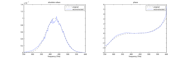
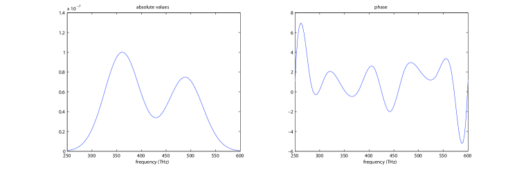
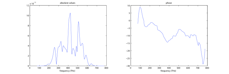
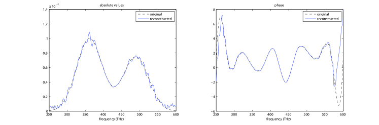
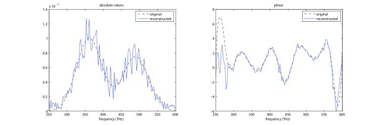
As a second example we have a more complex situation in mind. Here we choose an amplitude function with two peaks leading to the noisy function . The phase function shown in Figure 4(a) has more of a sinusoidal structure. Figure 4(b) again shows the result after the autoconvolution, this time without any noise. Even in this case we need an appropriate parameter to recover the phase in an acceptable way. The noise-free reconstruction is shown in Figure 4(c) with . While in the middle part both phases coincide nearly perfectly, problems arise at the boundaries as we already observed in the previous example. Because of the structure of the autoconvolution equation, the amount of information on the boundaries is much lower than in the middle, c.f. (26) and (27). The higher the noise level , the more severe those problems become. In the last figure a reconstruction for and is shown where a lot of noise artifacts remained. However, it seems that the absolute values are influenced more by the measurement errors than the phase. Numerical values for certain iterations are shown in Table 1. Especially our criterion to stop the iteration for fixed is clearly visible there. Namely, at , the difference of the absolute values of the iterate to the noisy reference values reaches its minimum. The solution at this iteration is the one shown in Figure 4(d).
7 Conclusions
In this paper, we have studied a new type of kernel-based autoconvolution problems, for which a stable approximate solution is required for measurements of ultrashort laser pulses with the self-diffraction SPIDER method. The problem is formulated as a nonlinear integral equation with complex-valued functions over a finite real interval on both sides of the equation. With respect to the mathematical model, the novelty of this inverse problem consists in the occurrence of a physically motivated complex kernel function and the observability of the amplitude of the incident pulse such that the focus of the paper is on phase reconstruction. After reviewing recent developments in ultrashort pulse characterization we have introduced an appropriate physical model (11) with kernel (12) and its mathematical description as a nonlinear operator equation. Using this abstract setting, which supports the mathematical analysis of the problem, we outlined by Example 3.1 the local ill-posedness of the inverse problem under consideration. That is, for given data the solution cannot be approximated arbitrarily precise, even if the noise on the data is sufficiently small. Titchmarsh’s convolution theorem formulated for our model in Lemma 4.1 enabled us to show that the autoconvolution equation has two complex conjugate solutions in case of a trivial kernel. However, the situation for arbitrary kernels seems to be an open question. A main goal of this article was to suggest and test an adapted regularization approach. We used a variant of the Levenberg-Marquardt algorithm (21) in the discretized form (30). A crucial point in the regularization process is the choice of the regularization parameter . Since the amplitude function can be measured as part of the solution, we could motivate a specific parameter choice rule (20). Under all regularized solutions, which are calculated for varying , we recommend to take the one that approximates the observed absolute values in an optimal way. It is known that iterates for regularized solutions to ill-posed problems tend to worsen whenever the iteration is not stopped early enough. To find an appropriate stopping rule, we monitored the deviation between the measured and calculated absolute values, which reaches a minimum during the iteration process and then increases again. This minimum is used to stop the iteration for fixed . Table 1 illustrates such behavior for some numerical example. Case studies with two different pulses and different noise levels indicate opportunities and limitations of our regularization method.
From a physicist’s point of view, the formalism described here opens a perspective for using a wider class of nonlinearities for the SPIDER pulse characterization method, making it more universally applicable. nonlinearities such as the self-diffraction process are much more widespread than processes that have been used nearly exclusively for SPIDER so far. With the solution of the SPIDER autoconvolution problem at hand, the integration of a complete optical pulse characterization set-up in an integrated optical device becomes feasible. As SPIDER is the only method that does not require mechanical variation of an optical delay this enables, in principle, the construction of an optical oscilloscope on chip, of course with the requirement to externally process the measured data by the discussed regularization procedure. Moreover, there appear other interesting applications of SPIDER variants for the characterization of broadband ultraviolet pulses, where processes do not offer viable options. For all these intriguing applications, we now demonstrated a viable way of retrieving the relevant phase data by regularization of the respective autoconvolution problem.
Acknowledgements
We thank four referees for reading the paper carefully. The given hints allowed us to state the aim of the paper more precisely. B. Hofmann was partly supported by Grant 1454/8-1 from Deutsche Forschungsgemeinschaft (DFG). D. Gerth was funded by the Austrian Science Fund (FWF): W1214-N15, project DK08. G. Steinmeyer gratefully acknowledges support by the Academy of Finland (Project Grant No. 128844).
References
- [1]
- [2] J. Baumeister, Deconvolution of appearance potential spectra, in Direct and inverse boundary value problems, Oberwolfach, 1989, Lang, Frankfurt am Main, 1991, pp. 1–13.
- [3] M. Richter, Approximation of Gaussian Random Elements and Statistics, Stuttgart, B. G. Teubner, 1992.
- [4] R. Gorenflo, B. Hofmann, On autoconvolution and regularization, Inverse Problems 10 (1994), pp. 353–373.
- [5] G. Fleischer, B. Hofmann, On inversion rates for the autoconvolution equation, Inverse Problems 12 (1996), pp. 419–435.
- [6] J. Janno, On a regularization method for the autoconvolution equation, Z. Angew. Math. Mech. 77 (1997), pp. 393–394.
- [7] J. Janno, Lavrent’ev regularization of ill-posed problems containing nonlinear near-to-monotone operators with application to autoconvolution equation, Inverse Problems 16 (2000), pp. 333–348.
- [8] G. Fleischer, R. Gorenflo, B. Hofmann, On the autoconvolution equation and total variation constraints, Z. Angew. Math. Mech. 79 (1999), pp. 149–159.
- [9] R. Ramlau, Morozov’s discrepancy principle for Tikhonov-regularization of nonlinear operators, Numer. Funct. Anal. Optim. 23 (2002), pp. 147–172.
- [10] K. Choi, A.D. Lanterman, An iterative deautoconvolution algorithm for nonnegative functions, Inverse Problems 21 (2005), pp. 981–995.
- [11] L. von Wolfersdorf, Autoconvolution equations and special functions, Integral Transforms Spec. Funct. 19 (2008), pp. 677–686.
- [12] Z. Dai, P.K. Lamm, Local regularization for the nonlinear inverse autoconvolution problem, SIAM J. Numer. Anal. 46 (2008), pp. 832–868.
- [13] S. Koke, S. Birkholz, J. Bethge, C. Grebing, G. Steinmeyer, Self-diffraction SPIDER, Conference on Lasers and Electro-Optics, OSA Technical Digest (CD) (Optical Society of America, 2010), paper CMK3, http://www.opticsinfobase.org/abstract.cfm?URI=CLEO-2010-CMK3.
- [14] H.W. Engl, M. Hanke, A. Neubauer, Regularization of Inverse Problems, Dordrecht, Kluwer, 1996.
- [15] A.N. Tikhonov, A.S. Leonov, A.G. Yagola, Nonlinear Ill-posed Problems. Vol. 1, 2, London, Chapman & Hall, 1998.
- [16] B. Kaltenbacher, A. Neubauer, O. Scherzer, Iterative Regularization Methods for Nonlinear Ill-Posed Problems, Berlin, Walter de Gruyter, 2008.
- [17] M.V. Klibanov, On the unique determination of a compactly supported function by the modulus of its Fourier transform, Soviet Math. Doklady 32 (1985), pp. 278–280.
- [18] M.V. Klibanov, P.E. Sacks, A.V. Tikhonravov, The phase retrieval problem, Inverse Problems 11 (1995), pp. 1–28.
- [19] T. Schuster, B. Kaltenbacher, B. Hofmann, and K.S. Kazimierski, Regularization Methods in Banach Spaces, Walter de Gruyter, Berlin – Boston, 2012.
- [20] M.V. Klibanov, Uniqueness of the determination of the distortions of a crystalline lattice by the X-ray diffraction method in a continuous dynamical model, Differential Equations 25 (1989), pp. 520–527.
- [21] M.V. Klibanov, P.E. Sacks, Use of partial knowledge of the potential in the phase problem of inverse scattering, J. Comput. Phys. 112 (1994), pp. 273–281.
- [22] M.V. Klibanov, On the recovery of a 2-D function from the modulus of its Fourier transform, J. Math. Anal. Appl. 323 (2006), pp. 818–843.
- [23] G. Steinmeyer, G. Stibenz, Generation of sub-4-fs pulses via compression of a white-light continuum using only chirped mirrors, Appl. Phys. B 82 (2006) pp. 175–181.
- [24] S. Rausch, T. Binhammer, A. Harth, F. X. Kärtner, U. Morgner, Few-cycle femtosecond field synthesizer, Opt. Exp. 16 (2008), pp. 17410–17419.
- [25] G. Krauss, S. Lohss, T. Hanke, A. Sell, S. Eggert, R. Huber, A. Leitenstorfer, Synthesis of a single cycle of light with compact erbium-doped fibre technology, Nature Photon. 4 (2010), pp. 33–36.
- [26] E. Goulielmakis, M. Schultze, M. Hofstetter, V. S. Yakovlev, J. Gagnon, M. Uiberacker, A. L. Aquila, E. M. Gullikson, D. T. Attwood, R. Kienberger, F. Krausz, U. Kleineberg, Single-cycle nonlinear optics, Science 320 (2008), pp. 1614–1617.
- [27] G. Sansone, E. Benedetti, F. Calegari, C. Vozzi, L. Avaldi, R. Flammini, L. Poletto, P. Villoresi, C. Altucci, R. Velotta, S. Stagira, S. De Silvestri, M. Nisoli, Isolated single-cycle attosecond pulses, Science 314 (2006), pp. 443–446.
- [28] J.A. Armstrong, Measurement of picosecond laser pulse widths, Appl. Phys. Lett. 10 (1967), pp. 16–18.
- [29] L. Gallmann, G. Steinmeyer, U. Keller, G. Imeshev, M. M. Fejer, J.P. Meyn, Generation of sub-6-fs blue pulses by frequency doubling with quasi-phase-matching gratings, Opt. Lett. 26 (2001), 614–616.
- [30] E.M. Hofstetter, Construction of time-limited functions with specialized autocorrelation functions, IEEE Trans. Inf. Theory IT-10 (1964) pp. 119- 126.
- [31] Yu.M. Bruck, L.G. Sodin, On the ambiguity of the image reconstruction problem, Opt. Commun. 30, (1979), pp. 304- 308.
- [32] K. Naganuma, K. Mogi, H. Yamada, General method of ultrashort light pulse chirp measurement, IEEE J. Quantum Electron. 25 (1989), pp. 1225- 1233.
- [33] J. Peatross, A. Rundquist, Temporal decorrelation of short laser pulses, J. Opt. Soc. Am. B 15 (1998), pp. 216–222.
- [34] K.-H. Honga, Y.S. Leeb, C.H. Namb, Electric-field reconstruction of femtosecond laser pulses from interferometric autocorrelation using an evolutionary algorithm, Opt. Commun. 271 (2007), pp. 169–177.
- [35] J.H. Chung, A.M. Weiner, Ambiguity of ultrashort pulse shapes retrieved from the intensity autocorrelation and the power spectrum, IEEE J. Sel. Top. Quantum Electron. 7 (2001), pp. 656–666.
- [36] R. Trebino, Frequency-Resolved Optical Gating: The Measurement of Ultrashort Laser Pulses, Boston, Kluwer, 2000.
- [37] D.T. Reid, Algorithm for complete and rapid retrieval of ultrashort pulse amplitude and phase from a sonogram, IEEE J. Quantum Electron. 35 (1999), pp. 1584–1589.
- [38] D. Keusters, H.S. Tan, P. O’Shea, E. Zeek, R. Trebino, W.S. Warren, Relative-phase ambiguities in measurements of ultrashort pulses with well-separated multiple frequency components, J. Opt. Soc. Am. B 20 (2003), pp. 2226–2237.
- [39] B. Seifert, H. Stolz, M. Tasche, Nontrivial ambiguities for blind frequency-resolved optical gating and the problem of uniqueness, J. Opt. Soc. Am. B 21 (2004), pp. 1089–1097.
- [40] E. Zeek, A.P. Shreenath, M. Kimmel, R. Trebino, Simultaneous Automatic Calibration and Direction-of-Time-Ambiguity Removal in Frequency-Resolved Optical Gating, Appl. Phys. B B74 (2002), pp. S265–S271.
- [41] K.W. DeLong, D.N. Fittinghoff, R. Trebino, B. Kohler, K. Wilson, Pulse retrieval in frequency-resolved optical gating based on the method of generalized projections, Opt. Lett. 19, (1994) pp. 2152-2154.
- [42] K.W. DeLong, D.N. Fittinghoff, and R. Trebino, Practical Issues in Ultrashort-Pulse Measurement Using Frequency-Resolved Optical Gating, IEEE J. Quantum Electron. 32 (1998), pp. 1253–1264.
- [43] I. Amat-Rold n, I.G. Cormack, P. Loza-Alvarez, D. Artigas, Measurement of electric field by interferometric spectral trace observation, Opt. Lett. 30, (2005), pp. 1063–1065.
- [44] D. Langemann, M. Tasche, Phase reconstruction by a multilevel iteratively regularized Gauss-Newton method Inverse Problems 24 (2008), 035006.
- [45] B. Seifert, H. Stolz, A method for unique phase retrieval of ultrafast optical fields, Meas. Sci. Technol. 20 (2009), 015303.
- [46] C. Iaconis, I.A. Walmsley, Spectral phase interferometry for direct electric-field reconstruction of ultrashort optical pulses Opt. Lett. 12, 792–794 (1998).
- [47] G. Steinmeyer, G. Stibenz, Optimizing spectral phase interferometry for direct electric-field reconstruction, Rev. Sci. Instrum. 77 (2006), 073105.
- [48] F. Reynaud, F. Salin, A. Barthelemy, Measurement of phase shifts introduced by nonlinear optical phenomena on subpicosecond pulses, Opt. Lett. 14 (1989), pp. 275–277.
- [49] D.N. Fittinghoff, J.L. Bowie, J.N. Sweetser, R.T. Jennings, M.A. Krumbügel, K.W. DeLong, R. Trebino, I.A. Walmsley, Measurement of the intensity and phase of ultraweak, ultrashort laser pulses, Opt. Lett. 21 (1996), pp. 884–886.
- [50] M. Takeda, H. Ina, S. Kobayashi, Fourier-transform method of fringe-pattern analysis for computer-based topography and interferometry, J. Opt. Soc. Am. 72 (1982), pp. 156–160.
- [51] J. Bethge, G. Steinmeyer, Numerical fringe pattern demodulation strategies in interferometry, Rev. Sci. Instrum. 79 (2008), 073102.
- [52] A. Pasquazi, M. Peccianti, Y. Park, B. E. Little, S. T. Chu, R. Morandotti, J. Azaña, D. J. Moss, Sub-picosecond phase-sensitive optical pulse characterization on a chip, Nature Photon. 5 (2011), pp. 618 -623.
- [53] V.L. Vinetskii, N.V. Kukhtarev, S.G. Odulov, M.S. Soskin, Dynamic self-diffraction of coherent light beams, Sov. Phys. Usp. 22 (1979), pp. 742–
- [54] Y.R. Shen, The Principles of Nonlinear Optics, John Wiley & Sons, 2003.
- [55] J. Liu, Y. Jiang, T. Kobayashi, R. Li, Z. Xu, Self-referenced spectral interferometry based on self-diffraction effect, J. Opt. Soc. Am. B 29 (2012), pp. 29–34.
- [56] T.I. Seidman, Nonconvergence results for the application of least-squares estimation to ill-posed problems, J. Optim. Theory Appl. 30 (1980), pp. 535–547.
- [57] R.D. Spies, K.G. Temperini, Arbitrary divergence speed of the least-squares method in infinite-dimensional inverse ill-posed problems, Inverse Problems 22 (2006), pp. 611–626.
- [58] B. Hofmann, O. Scherzer, Factors influencing the ill-posedness of nonlinear problems, Inverse Problems 10 (1994), pp. 1277–1297.
- [59] B. Hofmann, O. Scherzer, Local ill-posedness and source conditions of operator equations in Hilbert spaces, Inverse Problems 14 (1998), pp. 1189–1206.
- [60] B. Hofmann, Ill-posedness and local ill-posedness concepts in Hilbert spaces, Optimization 48 (2000), pp. 219–238.
- [61] D. Gerth, Regularization of an autoconvolution problem occurring in measurements of ultra-short laser pulses, Diploma thesis, Chemnitz University of Technology, Chemnitz, 2011.
- [62] E.C. Titchmarsh, The zeros of certain integral functions, Proc. London Math. Society 25 (1926), pp. 283–302.
- [63] S. Pohl, B. Hofmann, R. Neubert, T. Otto, C. Radehaus, A regularization approach for the determination of remission curves, Inverse Problems in Engineering 9 (2001), pp. 157–174.
- [64] A. B. Bakushinsky, M. Yu. Kokurin, A. Smirnova, Iterative Methods for Ill-Posed Problems – An Introduction, Walter de Gruyter, Berlin/New York, 2011.
- [65] M. Hanke, The regularizing Levenberg-Marquardt scheme is of optimal order, J. Integral Equations Appl. 22 (2010), 259–283.