Chiral magnetism and helimagnons in a pyrochlore antiferromagnet

Abstract

Recent neutron scattering measurements on the spinel CdCr₂O₄ revealed a rare example of helical magnetic order in geometrically frustrated pyrochlore antiferromagnet. The spin spiral characterized by an incommensurate wavevector $\mathbf{Q}=2\pi(0,\delta,1)$ with $\delta\approx 0.09$ is accompanied by a tetragonal distortion. Here we conduct a systematic study on the magnetic ground state resulting from the interplay between the Dzyaloshinskii-Moriya interaction and further neighbor exchange couplings, two of the most important mechanisms for stabilizing incommensurate spin orders. We compute the low-energy spin-wave spectrum based on a microscopic spin Hamiltonian and find a dispersion relation characteristic of the helimagnons. By numerically integrating the Landau-Lifshitz-Gilbert equation with realistic model parameters, an overall agreement between experiment and the numerical spectrum, lending further support to the view that a softened optical phonon triggers the magnetic transition and endows the lattice a chirality.

I Introduction

Magnets with geometrical frustration provide a fertile ground for studying complex spin orders and unconventional magnetic phases.moessner06 The defining feature of strong geometrical frustration is the occurrence of extensively degenerate ground states. This usually arises when the arrangement of spins on a lattice precludes satisfying all interactions at the same time. A great deal of attention has been devoted to the so-called pyrochlore magnets in which the magnetic ions form a three-dimensional connected network of corner-sharing tetrahedra.moessner98 With magnetic interactions restricted to only nearest neighbors, classical spins on the pyrochlore lattice remain disordered even at temperatures well below the Curie-Weiss energy scale. Magnetic fluctuations in this liquid-like phase are subject to strong local constraints that maintain vanishing total spin on each tetrahedron. This disordered yet highly correlated phase is often called a cooperative paramagnet. Because of the huge degeneracy, the magnet is sensitive to nominally small perturbations. The low-temperature ordering thus depends subtly on the residual perturbations present in the system.

The recent discovery of a novel chiral spin structure in spinel CdCr₂O₄ has generated much interest both theoretically and experimentally. chung05 ; matsuda07 The magnetic Cr ions in this compound have spin $S=3/2$ and no orbital degrees of freedom, providing a very good realization of Heisenberg antiferromagnet on the pyrochlore lattice. Despite a rather high Curie-Weiss temperature $|\Theta_{\rm CW}|\approx 70$ K, a spiral magnetic order sets in only at $T_{N}=7.8$ K, indicating a high degree of frustration. The discontinuous magnetic transition at $T_{N}$ is accompanied by a structural distortion which lowers the crystal symmetry from cubic to tetragonal ($a=b<c$) with an elongated unit cell: $(c-a)/c\approx 5\times 10^{-3}$. Polarized neutron-scattering experiment reveals an incommensurate magnetic order in which coplanar spins rotate about either $a$ or $b$ axes with a period of roughly ten lattice constants; the ordering wavevector $\mathbf{Q}=2\pi(0,\delta,1)$ with $\delta\approx 0.09$. It is worth noting that a very similar coplanar helical order has also been reported in the weak itinerant antiferromagnet YMn₂ ballou87 ; cywinski91 .

Spin-lattice coupling has been shown to play an important role in relieving magnetic frustrations in several chromium spinels. lee00 ; ueda06 ; matsuda07_Hg ; rudolf07 In particular, there are strong experimental evidences indicating that the magnetic transition in CdCr₂O₄ is mainly driven by spin-lattice coupling. These include anomalies of the elastic constants, bhattacharjee11 ; zherlitsyn10 splitting of optical phonons, valdes08 ; kant09 and energy shift of zone-boundary phonons kim11 at the magnetic ordering temperature. The spin-lattice or magnetoelastic coupling arises from the dependence of exchange on the ion displacements $\delta r_{ij}$ of spins: $(\partial J/\partial r)(\mathbf{S}_{i}\cdot\mathbf{S}_{j})\,\delta r_{ij}$. tcher02 ; chern09 As a result, the lattice distortion creates disparities between nearest-neighbor exchange constants and paves the way for magnetic ordering. However, spin-lattice coupling usually favors collinear magnetic orders. Indeed, assuming a simple elastic energy cost $k(\delta r_{ij})^{2}/2$ and integrating out the displacements $\delta r_{ij}$ in the above model gives rise to a biquadratic spin interaction: $-(\mathbf{S}_{i}\cdot\mathbf{S}_{j})^{2}$, which is minimized by collinear spins. While the magnetic frustration is relieved by the distortion, the appearance of helical spin order in CdCr₂O₄ thus comes from other mechanisms.

Magnetic spirals resulting from the competition between nearest neighbor and next nearest neighbor interactions are a common theme in frustrated spin systems. yoshimori59 ; adam80 However, this is not the case for pyrochlore lattice. Detailed mean-field and numerical investigations show that inclusion of further-neighbor interactions partially relieves the frustration and sometimes selects rather complicated multiple-$\mathbf{q}$ spin orders, but fails to stabilize magnetic spirals with a definite handedness. reimers91 ; chern08 Another mechanism for the formation of spirals is the Dzyaloshinskii-Moriya (DM) interaction which originates from the relativistic spin-orbit coupling. dzyaloshinskii64 ; moriya60 Although symmetry considerations allow the presence of DM terms in the pyrochlore lattice, elhajal05 the ground states selected by the DM interaction are non-chiral magnetic orders with wavevector $\mathbf{q}=0$. elhajal05 ; canals08 ; chern10

The origin of the spiral order as well as the lattice distortion in CdCr₂O₄ has been consistently explained in Ref. chern06, . In this scenario, the magnetic transition is triggered by the softening of $\mathbf{q}=0$ optical phonons with odd parity. The two types of tetrahedra with different orientations are flattened along the $a$ and $b$ directions, respectively, resulting in an overall tetragonal elongation along the $c$ axis. The lattice distortion relieves the magnetic frustration by creating disparities among the nearest-neighbor exchange constants and stabilizes a collinear Néel order with wavevector $\mathbf{Q}_{0}=2\pi(0,0,1)$. Moreover, the broken parity due to the staggered distortion gives rise to a chiral pyrochlore structure. The collinear spins are twisted into a long-period spiral with $\mathbf{Q}=2\pi(0,\delta,1)$ as the structural chirality is transferred to magnetic order by relativistic spin-orbit interaction.chern06 ; chern09 The broken parity in CdCr₂O₄ has also been confirmed by recent optical measurements. kant09

In this paper we undertake a systematic study of the general helical order resulting from the interplay between DM interaction and further-neighbor couplings in pyrochlore antiferromagnets. We also employ various numerical methods to investigate the spin-wave excitations in the spiral magnetic orders. We first revisit the continuum theory which is valid in the $J\to\infty$ limit and show that the resultant Hamiltonian possesses a continuous symmetry similar to that in smectic liquid crystals. deGennes93 ; chaikin ; radzihovsky11 In particular, despite the broken symmetry of the helical order is described by a O(3) order parameter, the three associated Goldstone modes reduce to a single smectic-like phonon mode which emerges on scales longer than the helical pitch. This low-energy gapless excitations, dubbed helimagnons in Ref. belitz06, , exhibit a highly anisotropic dispersion relation.

The emergent continuous symmetry of the effective theory is broken by the anisotropic crystal fields at the microscopic level. We first adopt the spherical approximation to investigate the resultant magnetic ground states. Three typical helical orders with wavevectors $(0,0,1-\delta)$, $(0,\delta,1)$ and $(\delta,\delta,1)$ are stabilized depending on the relative strengths of DM interaction $D$ and third neighbor interaction $J_{3}$. We then focus on the $(0,\delta,1)$ spiral, which is relevant to the case of CdCr₂O₄, and consider perturbation corrections to the coplanar spiral solution obtained from the continuum theory. We show that the first-order corrections do not shift the spiral pitch but introduces a small out-of-plane spin component.

Next we study the magnetic excitations in the spiral magnetic ground state. The incommensurate nature of the helical order presents a challenging task for the calculation of spin-wave spectrum. To circumvent this problem we employ the conventional Holstein-Primakoff method with a large commensurate unit cell. We also perform dynamics simulations based on the Landau-Lifshitz-Gilbert (LLG) equations. mochizuki10 The LLG simulations with a large damping also provide an efficient approach to obtain the accurate spin structures in the equilibrium state. The magnon spectrum obtained from our dynamics simulation exhibits a gapless mode at the helical wavevector $\mathbf{Q}=2\pi(0,\delta,1)$ reminiscent of the smectic-like phonon mode or helimagnons mentioned above. radzihovsky11 ; belitz06 An overall agreement is obtained between the numerical calculations and the experimental data on CdCr₂O₄.

The remainder of this paper is organized as follows. In Sec. II we consider the helical magnetic order in pyrochlore antiferromagnet. After presenting a minimal model relevant for CdCr₂O₄, we first review the continuum theory of the magnetic spirals on pyrochlore. We then demonstrate the existence of a continuous symmetry similar to that in smectic liquid crystals. We obtain a phase diagram of the helical order based on the spherical approximation. Sec. III is devoted to a discussion of the magnon excitations of pyrochlore magnet. A systematic analysis of the low-energy acoustic mode indicates a highly anisotropic dispersion characteristic of that of helimagnons. We then perform dynamics simulation to obtain the spin-wave spectrum of the helical spin order with wavevector $\mathbf{Q}=2\pi(0,\delta,1)$ and compare the results with available experimental data. We conclude in Sec. V with a summary and discussion of our results.

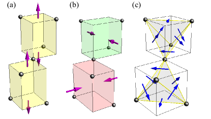
Figure 1: (Color online) Schematic picture of (a) even and (b) odd tetragonal distortions with $E_{g}$ and $E_{u}$ symmetries, respectively. Both types of distortion preserve the lattice translational symmetry and could result in an overall elongation along the $c$ axis. Panel (c) shows the DM vectors $\mathbf{D}_{ij}$ on the six inequivalent NN bonds of the pyrochlore lattice.

II Helical magnetic order

Our starting point is a classical Heisenberg model on the pyrochlore lattice described by the Hamiltonian

$$\mathcal{H} = \sum_{\langle ij\rangle}\left(J+K_{ij}\right)\,{\bf S}_{i}\cdot{\bf S}_{j}+\sum_{\langle ij\rangle}{\bf D}_{ij}\cdot\left({\bf S}_{i}\times{\bf S}_{j}\right)$$ (1)

$$+\,\,J_{2}\sum_{\langle\langle ij\rangle\rangle}\mathbf{S}_{i}\cdot\mathbf{S}_{j}+J_{3}\sum_{\langle\langle\langle ij\rangle\rangle\rangle}\mathbf{S}_{i}\cdot\mathbf{S}_{j},$$

The dominant term is the nearest-neighbor (NN) exchange interaction with an antiferromagnetic sign $J>0$. Due to the special geometry of the pyrochlore lattice, this term can be recast to $(J/2)\sum_{\mathbf{r}}\left|\mathbf{M}(\mathbf{r})\right|^{2}$, where $\mathbf{M}$ denotes the vector sum of spins on a tetrahedron at $\mathbf{r}$. Minimization of this term requires the vanishing of total magnetic moment on every tetrahedron but leaves an extensively degenerate manifold.

The exchange anisotropy $K_{ij}$ results from a distorted lattice through magnetoelastic coupling. The structural distortion in CdCr₂O₄ reduces the crystal symmetry from cubic to tetragonal while preserving the lattice translational symmetry. chung05 Here we consider $\mathbf{q}=0$ lattice distortions with even and odd parities; see Fig. 1(a) and (b). The dominant $E_{u}$ component results in a staggered distortion: tetrahedra of types I and II are flattened along the $a$ and $b$ directions, respectively; the lattice is elongated overall, $a=b<c$. The resulting space group, $I4_{1}22$, lacks the inversion symmetry. Fig. 2 shows the exchange anisotropy of the six NN bonds in the unit cell. As pointed out in Ref. tcher02, , this tetragonal distortion completely relieves the magnetic frustration and stabilizes a collinear Néel order with wavevector $\mathbf{Q}_{0}=2\pi(0,0,1)$ shown in Fig. 2.

The DM term $\mathbf{D}_{ij}\cdot(\mathbf{S}_{i}\times\mathbf{S}_{j})$ originates from the relativistic spin-orbit interaction $\lambda(\mathbf{L}\cdot\mathbf{S})$. This term is allowed on the ideal pyrochlore lattice, where the bonds are not centrosymmetric as required by the so-called Moriya rules. moriya60 Moreover, the high symmetry of the pyrochlore lattice completely determines the orientations of the DM vectors [see Fig. 1(c)] up to a multiplicative factor. Finally, we also include second and third exchanges couplings $J_{2}$ and $J_{3}$, respectively, in the model Hamiltonian. First principle ab initio calculations indicate that these further-neighbor exchanges are important for the modeling of spinel CdCr₂O₄. chern06 ; yaresko08 In the limit dominated by a large NN exchange, the ground-state properties actually depend only on the difference between $J_{2}$ and $J_{3}$. The relative shift in energy for any pair of ground states due to a small $J_{3}$ is identical to the effect of a $J_{2}$ of the same magnitude with an opposite sign. chern08

II.1 Gradient approximation and emergent continuous symmetry

We first briefly review the continuum theory of helical orders derived from the $\mathbf{Q}_{0}=2\pi(0,0,1)$ Néel order. The effective energy functional is obtained based on a gradient approximation of the staggered magnetizations.chern06 ; chern09 The antiferromagnetic order on the pyrochlore lattice is characterized by three order parameters:

$$\mathbf{L}_{1} = (\mathbf{S}_{0}+\mathbf{S}_{1}-\mathbf{S}_{2}-\mathbf{S}_{3})/4,$$

$$\mathbf{L}_{2} = (\mathbf{S}_{0}-\mathbf{S}_{1}+\mathbf{S}_{2}-\mathbf{S}_{3})/4,$$ (2)

$$\mathbf{L}_{3} = (\mathbf{S}_{0}-\mathbf{S}_{1}-\mathbf{S}_{2}+\mathbf{S}_{3})/4,$$

where $\mathbf{S}_{\mu}$ denotes magnetic moments at $\mu$th sublattice. chern06 For example, the collinear Néel state shown in Fig. 2 is described by order parameters: $\mathbf{M}=0$, $\mathbf{L}_{2}=\mathbf{L}_{3}=0$, and $\mathbf{L}_{1}={\hat{\mathbf{n}}}_{1}\,e^{i\mathbf{Q}_{0}\cdot\mathbf{r}}$, where ${\hat{\mathbf{n}}}_{1}$ is an arbitrary unit vector. Assuming a slow variation of staggered magnetizations in the low-period spiral, we parameterize the order parameters as: $\mathbf{L}_{i}(\mathbf{r})=e^{i\mathbf{q}\cdot\mathbf{r}}\phi_{i}(\mathbf{r})\,\hat{\mathbf{n}}_{i}(\mathbf{r})$, where $\mathbf{n}_{i}(\mathbf{r})$ and $\phi_{i}(r)$ are the directions and magnitudes of the staggered magnetizations. The hard constraints $|\mathbf{S}_{i}|=S$ require that three unit vectors $\hat{\mathbf{n}}_{i}$ are orthogonal to each other and $\phi_{1}^{2}+\phi_{2}^{2}+\phi_{3}^{2}=1$. chern06 Note that the phase factor $e^{i\,\mathbf{Q}_{0}\cdot\mathbf{r}}=\pm 1$ changes sign between consecutive layers of tetrahedra along the $z$ direction (cf. the two layers of green tetrahedra in Fig. 3).

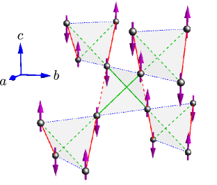
Figure 2: (Color online) A Néel order on the pyrochlore lattice with wavevector $\mathbf{q}=2\pi(0,0,1)$. This collinear spin order is stabilized by a staggered distortion with $E_{u}$ symmetry. Tetrahedra of type I and II are flattened along the $a$ and $b$ directions, respectively. The exchange constants on various NN bonds are $J+K_{u}-K_{g}$ (solid), $J-2K_{u}-K_{g}$ (dashed), and $J+K_{u}+2K_{g}$ (dotted).

The calculation can be further simplified in the $J\to\infty$ limit. The vanishing of the total magnetization on tetrahedra in this limit requires $\hat{\mathbf{n}}_{3}\parallel\partial_{y}\hat{\mathbf{n}}_{1}$, and the $\phi$ fields can be analytically expressed in terms of the director fields $\hat{\mathbf{n}}_{i}$. The effective energy functional in the gradient approximation can be solely expressed in terms of the director fields $\hat{\mathbf{n}}_{1}$ and $\hat{\mathbf{n}}_{2}\parallel\partial_{y}\hat{\mathbf{n}}_{1}\times\hat{\mathbf{n}}_{1}$ chern06 . It contains two contributions: $\mathcal{F}=\int d\mathbf{r}\left(E_{K}+E_{DM}\right)$. The first term, originating from magnetoelastic coupling, gives penalties to variations of the staggered magnetizations:

$$E_{K}=\frac{K_{u}}{4}\Bigl{[}\left(\partial_{x}\hat{\mathbf{n}}_{1}\right)^{2}+\left(\partial_{y}\hat{\mathbf{n}}_{1}\right)^{2}+2\left(\partial_{z}\hat{\mathbf{n}}_{1}\right)^{2}-\left(\hat{\mathbf{n}}_{2}\cdot\partial_{z}\hat{\mathbf{n}}_{1}\right)^{2}\Bigr{]},\\$$

while the DM term contains Lifshitz invariants which are first-order in the gradients of $\hat{\mathbf{n}}_{1}$:

$$E_{DM}=-D\hat{\mathbf{n}}_{1}\cdot\bigl{(}\hat{\mathbf{a}}\times{\partial_{x}\hat{\mathbf{n}}_{1}}+\hat{\mathbf{b}}\times{\partial_{y}\hat{\mathbf{n}}_{1}}-\hat{\mathbf{c}}\times{\partial_{z}\hat{\mathbf{n}}_{1}}\bigr{)}/4.\quad$$ (3)

Here we orient the axes of coordinate reference frame $x,y,$ and $z$ along the principal axes $a,b$, and $c$ of the crystal.

The form of the DM functional suggests spiral solutions with $\hat{\mathbf{n}}_{1}$ rotating about one of the principal axes and staying in the plane perpendicular to it. These special solutions were first obtained in Ref. chern06, . For example, the solution $\hat{\mathbf{n}}_{1}=(\cos\theta(y),0,\sin\theta(y))$ with $\theta(y)=2\pi\delta y+\psi$ describes a helical order with coplanar spins lying in the $ac$ plane (see Fig. 3). This spiral magnetic order producing a Bragg scattering at $\mathbf{Q}=2\pi(0,\delta,1)$ is consistent with the experimental characterization of CdCr₂O₄. chung05

The energy functional $\mathcal{F}$ actually possesses a continuous symmetry related to the O(2) rotational invariance of the helical axis. To describe the general coplanar spiral solution, we first introduce two orthogonal unit vectors lying in the $xy$ plane:

$$\hat{\bm{\xi}} = +\cos\Phi\,\hat{\mathbf{x}}+\sin\Phi\,\hat{\mathbf{y}},$$

$$\hat{\bm{\zeta}} = -\sin\Phi\,\hat{\mathbf{x}}+\cos\Phi\,\hat{\mathbf{y}}$$ (4)

A coplanar spiral with spins rotating about the $\hat{\bm{\xi}}$ direction has the form

$$\hat{\mathbf{n}}_{1}(\mathbf{r})=\cos\theta(\xi)\,\hat{\bm{\zeta}}+\sin\theta(\xi)\,\hat{\mathbf{z}},\qquad\xi\equiv\mathbf{r}\cdot\hat{\bm{\xi}}.$$ (5)

Substituting $\hat{\mathbf{n}}_{1}(\mathbf{r})$ into the Eqs. (II.1) and (3) yields an energy density: $E[\theta]=-D\partial_{\xi}\theta+\frac{1}{4}K_{u}\left(\partial_{\xi}\theta\right)^{2},$ whose minimization gives a helical wavenumber

$$\mathcal{Q}=2\pi\delta=d\theta/d\xi=2D/K_{u}.$$ (6)

The O(2) invariance indicates that the magnetic energy is independent of the angle $\Phi$, i.e. $\delta\mathcal{F}[\hat{\mathbf{n}}_{1}]/\delta\Phi=0$. It is worth noting that this degeneracy is similar to the O(3) symmetry for the helical axis observed in the spiral order of MnSi. belitz06 More importantly, as will be discussed below, it is exactly this additional symmetry that gives rise to the anisotropic dispersion of helimagnons.

The coplanar spirals described above (with its axis lying in the $xy$ plane) are also accidentally degenerate with a spiral in which spins rotate about the $z$ axis. chern06 In real compounds, this accidental degeneracy as well as the aforementioned O(2) symmetry are lifted by further neighbor interactions and cubic symmetry field of the lattice. In particular, the further-neighbor exchange contributes to a gradient term $(J_{3}-J_{2})(\partial_{z}\hat{\mathbf{n}}_{1})^{2}$ in the gradient expansion. chern06 The experimentally observed $(0,\delta,1)$ spiral is selected by a large antiferromagnetic third-neighbor exchange $J_{3}$ which favors coplanar spirals rotating about the $x$ or $y$ axes. The explicit magnetizations of a spiral with the pitch vector parallel to the $y$-axis are

$${\bar{\mathbf{S}}}_{\mu}(\mathbf{r})=\hat{\mathbf{a}}\,\sin(\mathbf{Q}\cdot\mathbf{r}+\varphi_{\mu})+\hat{\mathbf{c}}\,\cos(\mathbf{Q}\cdot\mathbf{r}+\varphi_{\mu}),$$ (7)

where $\mu=0,1,2,3$ is the sublattice index, $\varphi_{0}=\psi$, $\varphi_{1}=\pi\delta+\psi$, $\varphi_{2}=\pi+\psi$, and $\varphi_{3}=\pi(1+\delta)+\psi$, with $\psi$ an arbitrary constant related to the U(1) symmetry of the coplanar spiral, i.e. $\theta(\mathbf{r})=\mathbf{Q}\cdot\mathbf{r}+\psi$.

It is worth noting that the pitch of magnetic spirals induced by DM interaction is usually rather long with the wavenumber of the order $\delta\sim D/J\sim 10^{-3}-10^{-2}$. The relatively short pitch of spirals in CdCr₂O₄ is due to the ineffectualness of $J$ in stabilizing the magneitc order. Instead, the DM interaction competes with the magnetoelastic coupling and the helical wavenumber is given by $\delta\sim D/K\approx 0.1$.

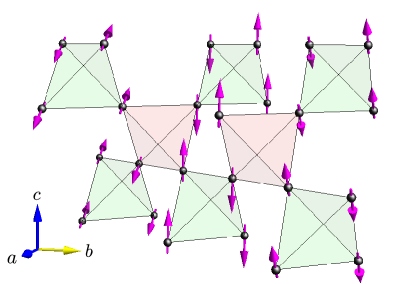
Figure 3: (Color online) Coplanar helical order with spins lying in the $ac$ plane and rotating about the $b$ axis. The magnetic order corresponds to the solution $\hat{\mathbf{n}}_{1}=(\cos\theta(y),0,\sin\theta(y))$, with $\theta(y)=2\pi\delta y+\mbox{const}$. It produces a Bragg peak $\mathbf{Q}=2\pi(0,\delta,1)$ in neutron scattering, consistent with the experimental measurement on CdCr₂O₄.

II.2 Spherical approximation

While the above continuum theory gives a rather consistent and simple picture of helical magnetic orders in tetragonal pyrochlore antiferromagnets, it is based on the assumption of an infinite $J$. To go beyond this limit and investigate the magnetic orders when the various parameters are of similar order, we resort to the spherical approximation, in which the local length constraints $|\mathbf{S}_{i}|=S$ are replaced by a global one $\sum_{i=1}^{N}|\mathbf{S}_{i}|^{2}=NS^{2}$, where $N$ is the number of lattice sites. With this soft constraint, the model Hamiltonian (1) can be diagonalized with the aid of Fourier transform $\mathbf{S}_{i}=\sum_{\mathbf{k}}\mathbf{S}_{\mu}(\mathbf{k})\,e^{i\mathbf{k}\cdot\mathbf{r}}$. Here we label a lattice site as $i=(\mu,\mathbf{r})$, where $\mu=0,1,2,3$ is the sublattice index and $\mathbf{r}$ denotes its position. The Hamiltonian then becomes

$$\mathcal{H} = \sum_{\mathbf{k}}\sum_{\mu,\nu}J_{\mu\nu}(\mathbf{k})\,\mathbf{S}_{\mu}(\mathbf{k})\cdot\mathbf{S}_{\nu}(-\mathbf{k})$$ (8)

$$+ \sum_{\mathbf{k}}\sum_{\mu,\nu}\sum_{\alpha,\beta}\,D^{\alpha\beta}_{\mu\nu}(\mathbf{k})S^{\alpha}_{\mu}(\mathbf{k})\,S^{\beta}_{\nu}(-\mathbf{k}),$$

where the matrices $J_{\mu\nu}(\mathbf{k})$ and $D^{\alpha\beta}_{\mu\nu}(\mathbf{k})$ are the Fourier transform of the exchange and DM interactions, respectively. The explicit form of the matrices are given in the Appendix A. The ground-state energy is given by the minimum eigenvalue $\lambda_{\rm min}$ of the matrix $H^{\alpha\beta}_{\mu\nu}=J_{\mu\nu}\delta^{\alpha\beta}+D^{\alpha\beta}_{\mu\nu}$. In particular, the ordering wavevector $\mathbf{Q}$ is obtained by minimizing $\lambda_{\rm min}(\mathbf{k})$ with respect to $\mathbf{k}$, i.e. $E_{0}=N\lambda_{\rm min}(\mathbf{Q})$.

Fig. 4 shows the ordering wavevector $\mathbf{Q}$ as a function of DM interaction and third-neighbor coupling $J_{3}$. We find three different helical orders characterized by an incommensurate wavenumber $\delta\sim D/K_{u}$. At small $J_{3}$, the ordering wavevector $\mathbf{Q}=2\pi(0,0,1-\delta)$ indicates a magnetic spiral in which spins rotate about the $z$ axis. This spiral solution has been discussed in Ref. chern06, and is accidentally degenerate with the coplanar spirals described in Eq. (7) in the $J\to\infty$ limit. A new spiral order with ordering wavevector $\mathbf{Q}=2\pi(\delta,\delta,1)$ is obtained for a small window of $J_{3}$ (depending on the value of $K_{u}$). This spiral state with its axis pointing along the diagonal in the $xy$ plane is also included in the general coplanar spiral solution Eq. (5) in the infinite $J$ limit. As $J_{3}$ is further increased, the $(0,\delta,1)$ spiral observed in CdCr₂O₄ becomes the ground state. For a helical wavenumber $\delta\sim 0.1$, this spiral order is indeed the magnetic ground state for a $J_{3}\approx 0.3J$, consistent with the ab initio calculations. chern06 ; yaresko08

Interestingly, for small exchange anisotropies, e.g. $K_{u}=0.1J$, the spiral order $(0,\delta,1)$ with axis along either $a$ or $b$ axes is sandwiched by the spiral state with axis along the $[110]$ direction, and the ordering wavevector $\mathbf{Q}$ switches back to $2\pi(\delta,\delta,1)$ for largest $J_{3}$ [Fig. 4(a)]. On the other hand, for larger anisotropy $K_{u}$, the ground state remains the $(0,\delta,1)$ spiral for large $J_{3}$.

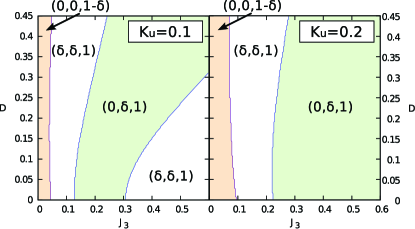
Figure 4: (Color online) Phase diagram of helical magnetic orders on pyrochlore lattice based on spherical approximation. Both $D$ and $J_{3}$ are measured with respect to the NN exchange $J$, and we have set the odd-parity exchange anisotropy $K_{u}=0.1J$ and $0.2J$ while leaving the even-parity exchange anisotropy $K_{g}=0$. The green, yellow, and white regions are characterized by a ordering wavevector $\mathbf{Q}=2\pi(0,\delta,1)$, $2\pi(0,0,1-\delta)$, and $2\pi(\delta,\delta,1)$, respectively.

II.3 Perturbation correction to coplanar spirals

We now focus on the helical magnetic order with wavevector $\mathbf{Q}=2\pi(0,\delta,1)$, which is relevant for the case of CdCr₂O₄, and use perturbation method to obtain corrections $\mathbf{s}_{i}\sim\mathcal{O}(D/J)$ to the coplanar spiral solution Eq. (7) when the NN exchange is finite. In the ground state, the magnetic moment is parallel or antiparallel to the effective exchange field

$$\mathbf{H}_{i}=\partial\mathcal{H}/\partial\mathbf{S}_{i}=\sum_{j}\left(J_{ij}\,\mathbf{S}_{j}-\mathbf{D}_{ij}\times\mathbf{S}_{j}\right),$$ (9)

such that the torque $\mathbf{T}_{i}=\mathbf{S}_{i}\times\mathbf{H}_{i}$ vanishes. Mathematically, our perturbative calculation is based on a $1/J$ expansion of the equilibrium equation $\mathbf{T}_{i}=0$. The zeroth-order result corresponds to the $J\to\infty$ limit and is given by Eq. (7). We express the exchange field as $\mathbf{H}_{i}=\bar{\mathbf{H}}_{i}+\mathbf{h}_{i}$, the condition of zero torque requires

$$({\bar{\mathbf{S}}}_{i}+\mathbf{s}_{i})\times({\bar{\mathbf{H}}}_{i}+\mathbf{h}_{i})=0.$$

Collecting only terms linear in $D/J$ from this equation, we obtain a set of coupled equations:

$$\qquad\qquad\quad\sum_{j}J_{ij}\cos\theta_{ij}\,(s^{x}_{i}-s_{j}^{x})=0,$$ (10)

$$\!\!\!\!\!\sum_{j}\left\{D_{ij}^{x}\cos\theta_{j}-D_{ij}^{z}\sin\theta_{j}-J_{ij}\left[\cos\theta_{ij}\,s_{i}^{y}-s_{j}^{y}\right]\right\}=0,$$

where $\theta_{i}={\bf Q}\cdot{\bf r}+\psi_{\mu}$, and $\theta_{ij}=\theta_{i}-\theta_{j}$. Sine the NN exchange $J$ can be expressed as $(J/2)|\mathbf{M}(\mathbf{r})|^{2}$, the $J\to\infty$ limit imposes hard constraints $\mathbf{M}(\mathbf{r})=0$ on all tetrahedra. A finite value of $J$ is thus expected to introduce a finite total magnetization. For simplicity, here we consider anisotropies dominated by a tetragonal distortion with odd parity only. Solving the above equations yields ($\mu=0,\cdots,3$)

$$\mathbf{s}_{\mu}(\mathbf{r})=\frac{-\sqrt{2}D}{(4J+10K_{u})}\,\cos\left(\mathbf{Q}\cdot\mathbf{r}\right)\,\hat{\mathbf{b}}.$$ (12)

Interestingly, the first-order corrections does not modify the spiral pitch; the incommensurate ordering wavevector is still given by the zeroth order expression $\mathcal{Q}=2\pi\delta$. As the correction is uniform for the four sublattices, the finite value of $J$ gives rise to a modulated ferromagnetic component $\mathbf{M}(\mathbf{r})$ on individual tetrahedron.

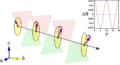
Figure 5: (Color online) A schematic diagram showing the out-of-plane corrections to a coplanar helical order. The coplanar spins are described by a vector field $\hat{\mathbf{n}}_{1}=(\cos\theta(y),0,\sin\theta(y))$, with $\theta(y)=2\pi\delta y+\mbox{const}$, while the out-of-plane components are given by Eq. (12). The inset shows the out-of-plane spin component $\Delta\mathbf{S}$ as a function of $r$ computed for the following set of parameters: $J=1.35\mbox{~{}meV}$, $K_{u}=0.21\mbox{~{}meV}$, $K_{g}=0\mbox{~{}meV}$, $D=0.14\mbox{~{}meV}$, and $J_{3}=0.28\mbox{~{}meV}$.

II.4 Relaxation dynamics simulations

While the perturbation correction gives a better approximation of the helical order in pyrochlore lattice, a high-precision description of the magnetic structure is required for the calculation of spin-wave excitations. A common approach to obtain the magnetic ground state is the low-temperature Monte Carlo simulations. However, the spin configurations obtained from Monte Carlo simulations are still too noisy for the purpose of the calculation of magnon spectrum. Instead, here we resort to the overdamped dynamics simulations based on the Landau-Lifshitz-Gilbert (LLG) equations. In particular, since the coplanar spiral solution with the perturbation corrections already provide a close approximation to the true ground state, such relaxation simulations can efficiently bring the system to the desired magnetic order.

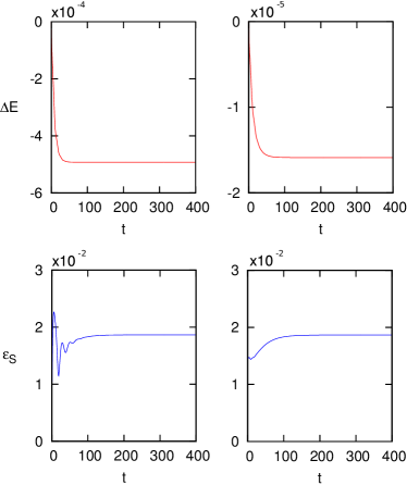
Figure 6: (Color online) The energy decrease $\Delta E(t)=E(t)-E(t=0)$ as a function of simulation time starting with (a) coplanar spiral solution Eq. (7) and (b) initial state including first order correction (12). The energy and time are measured with respect to $J$ and $1/J$, respectively. We performed the simulations on a lattice with $16\times 10^{3}$ spins with periodic boundary conditions. Panels (c) and (d) show the corresponding averaged spin deviations $\epsilon_{S}(t)=\sum_{i}|{\bf S}_{i}(t)-{\bar{\mathbf{S}}}_{i}|/N$ from the coplanar state and the inclusion of the first order correction respectively as a function of simulation time.

The LLG equation is a first-order differential equation describing the dynamics of classical magnetic moments:

$$\frac{\partial\mathbf{S}_{i}}{\partial t}=\mathbf{S}_{i}\times\mathbf{H}_{i}+\frac{\alpha_{G}}{S}\mathbf{S}_{i}\times\frac{\partial\mathbf{S}_{i}}{\partial t},$$ (13)

where $\mathbf{H}_{i}$ is the effective exchange field defined in Eq. (9), and $\alpha_{G}$ is a dimensionless damping parameter. We employ a finite-difference method to integrate the LLG equation numerically. serpico01 The technical details of the numerical method can be found in Appendix B. We performed our simulations on a cluster of $10^{3}$ cubic unit cells with $N=16000$ spins. Periodic boundary conditions were used in all simulations. We have also tested our algorithms on some well studied Hamiltonians and obtained excellent agreement with exact solutions.

We start our dynamics simulation from the coplanar spiral state both with and without the first-order corrections. Fig. 6 shows the simulation results for parameters $K_{u}=0.1J$, $D=-0.069J$ and $J_{3}=0.2J$; the corresponding helical wavenumber is $\delta=0.1$. In both cases, the energy monotonically decreases with simulation time, indicating a steady relaxation towards the true helical magnetic ground state. Also shown are the averaged deviations of spin configurations $\mathbf{S}_{i}(t)$ from the coplanar helical state (with and without first-order correction) as a function of simulation time. The rather small deviations of the order $10^{-2}$ indicate that both the coplanar spiral and the first-order result are indeed already good approximations to the ground state. Fig. 7 shows the structure factor $\mathcal{S}(\mathbf{k})=\left|(1/N)\sum_{i}\mathbf{S}_{i}\exp({i\mathbf{k}\cdot\mathbf{r}_{i}})\right|^{2}$ of the spin configurations obtained from the relaxation dynamics simulations. As expected, the structure factor exhibits peaks at the ordering wavevector $\mathbf{Q}=2\pi(0,\delta,1)$.

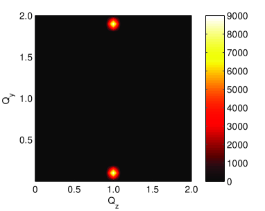
Figure 7: (Color online) Structure factor of the helical spin order obtained from the relaxation dynamics simulation. Sharp peaks appear at the ordering wavevector ${\bf Q}=2\pi(0,\delta,1)$.

III Spin-wave excitations

In this Section we study magnetic excitations of the helical magnetic order on the pyrochlore lattice. We first discuss the so-called helimagnons in the continuum limit. The appearance of this special gapless mode originates from the unique symmetry-breaking in chiral magnets. However, since the spiral pitch in CdCr₂O₄ is relatively short compared with helical orders in other systems, the crystal effects are expected to modify the helimagnon dispersion significantly. We thus also compute the spin-wave dispersions based on microscopic spin models. Starting from the high-precision ground state obtained in the previous section, we performed exact diagonalizations on a large unit cell to study the nature of the low-energy acoustic-like modes. The results are then compared with the predictions based on helimagnon theory. We also employed dynamics simulations on finite systems to obtain the full magnon spectrum and compare the results with the experiments.

III.1 Helimagnons in the continuum limit

We first consider magnetic fluctuations in the helical order within the framework of the continuum theory. For a spiral with a fixed axis, the obvious soft modes are phase fluctuations associated with the coplanar director field. More specifically, let us consider a spiral with its axis along the $y$-direction: $\hat{\mathbf{n}}_{1}=(\cos\theta,0,\sin\theta)$. Introducing a slowly-varying perturbation to the phase angle $\theta=\mathcal{Q}y+\psi(\mathbf{r})$, the energy functional associated with the fluctuations is $\mathcal{E}[\psi]=K_{u}\int d\mathbf{r}\left[\nabla\psi(\mathbf{r})\right]^{2}$. This indeed describes a soft mode similar to that of a planar magnet. However, as is well known in chiral nematics and smectic liquid crystals, a phase fluctuation of the form $\psi=\alpha\,\zeta$ corresponds to a simple rotation of the helical axis. chaikin Since coplanar spirals with different axes are energetically degenerate (see discussions in Sec. II.1), such rotations cannot cost energy, yet $\mathcal{E}\sim\alpha^{2}\neq 0$ for this particular phase fluctuation. Consequently, there cannot be any $(\partial_{\zeta}\psi)^{2}$ term in the effective energy density. The correct energy functional thus has the form chaikin ; belitz06

$$\mathcal{E}=\frac{1}{2}\!\int\!d\mathbf{r}\Bigl{[}c_{z}\!\left(\partial_{z}\psi\right)^{2}+\!c_{\parallel}\!\left(\partial_{\xi}\psi\right)^{2}+\!\frac{c_{\perp}}{\mathcal{Q}^{2}}\!\left(\partial^{2}_{\zeta}\psi\right)^{2}\!\Bigr{]},\,\,$$ (14)

where $c_{\parallel}$, $c_{\perp}\sim K_{u}$, $c_{z}\sim J_{3}$ are elastic constants, and $\mathcal{Q}=2\pi\delta$ is the pitch wavenumber. Note that the first term in the above equation arises from a rather large $J_{3}$ which gives a penalty to variations along the $z$ direction.

A derivation of the dynamics equations starting from the microscopic model (1) is tedious and almost intractable. To obtain the dispersion of the soft mode, it is more illuminating to employ a simple phenomenological approach based on the time-dependent Ginzburg-Landau theory. chaikin ; belitz06 In this formalism, the Goldstone mode $\psi$ couples to a mode $m$ at zero wavevector, which is soft due to spin conservation. Schematically the coarse-grained magnetization field is

$$\mathbf{S}_{\mu}(\mathbf{r})\sim{\bar{\mathbf{S}}}_{\mu}(\mathbf{r})\,+\,m(\mathbf{r})\hat{\mathbf{y}}$$ (15)

$$\quad+\,\,\psi(\mathbf{r})\,\bigl{[}\cos(\mathbf{Q}\cdot\mathbf{r}+\varphi_{\mu})\,\hat{\mathbf{x}}-\sin(\mathbf{Q}\cdot\mathbf{r}+\varphi_{\mu})\,\hat{\mathbf{z}}\bigr{]},$$

where ${\bar{\mathbf{S}}}_{\mu}$ is the coplanar spiral given in Eq. (7) and $\varphi_{\mu}$ denotes the relative phase shift of the sublattices. The total energy functional becomes

$$\mathcal{F}[m,\psi]=\frac{r_{0}}{2}\int d\mathbf{r}\,m^{2}(\mathbf{r})+\mathcal{E}[\psi].$$ (16)

Here $r_{0}$ is an effective mass of the zero-wavevector mode. The magnetization dynamics is governed by a generalized Landau-Lifshitz equation:

$$\partial_{t}\mathbf{S}_{\mu}(\mathbf{r})=-\gamma\,\mathbf{S}_{\mu}(\mathbf{r})\times\frac{\delta\mathcal{F}}{\delta\mathbf{S}_{\mu}(\mathbf{r})}$$ (17)

where $\gamma$ is a constant. Substituting (15) into the above equation and following similar steps outlined in Ref. belitz06, , we arrive at the following coupled equations

$$\partial_{t}m(\mathbf{r})=-\gamma\frac{\delta\mathcal{F}}{\delta\psi(\mathbf{r})},\qquad\partial_{t}\psi(\mathbf{r})=\gamma\frac{\delta\mathcal{F}}{\delta m(\mathbf{r})}.$$ (18)

To obtain the spectrum of the soft mode, we eliminate $m$ in the above equations to obtain a wave equation for the $\psi$ field

$$\partial_{t}^{2}\psi(\mathbf{r})=-r_{0}\gamma^{2}\left(-c_{z}\partial_{z}^{2}-c_{\parallel}\partial_{\xi}^{2}+\frac{c_{\perp}}{\mathcal{Q}^{2}}\partial_{\zeta}^{4}\right)\psi(\mathbf{r}).$$ (19)

Assuming a space-time dependence $\psi\sim\exp(i\mathbf{k}\cdot\mathbf{r}-i\epsilon_{\mathbf{k}}t)$, the energy of the soft mode is

$$\epsilon(\mathbf{k})=\gamma\,r_{0}^{1/2}\,\sqrt{c_{z}k_{z}^{2}+c_{\parallel}k_{\parallel}^{2}+\frac{c_{\perp}}{\mathcal{Q}^{2}}k_{\perp}^{4}}.$$ (20)

The dispersion is highly anisotropic: for wavevectors parallel to the spiral $\xi$-axis direction or the $z$-axis the dispersion is linear as in an antiferromagnet, while it is quadratic for wavevectors parallel to the $x$-axis.

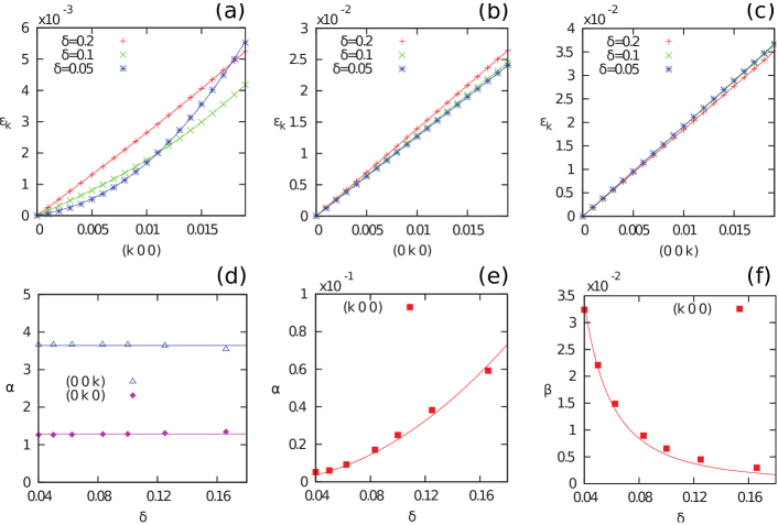
Figure 8: (Color online) Spin-wave dispersions along three principal axes [panels (a)–(c)] obtained from numerical exact diagonalization of a large unit cell. The results are fitted to the phenomenological dispersion $\epsilon_{\mathbf{k}}=\sqrt{\alpha k^{2}+\beta k^{4}}$. The magnon energy is measured in unit of $JS$. Panels (d)–(f) show the dispersion parameters $\alpha$ and $\beta$ as a function of the helical wavenumber $\delta$. These data are fitted to $\alpha=$const, $\alpha\propto\delta^{2}$, and $\beta\propto\delta^{-2}$, respectively.

III.2 Exact diagonalization with large unit cell

As discussed in Sec. II.1, the helical wavenumber in tetragonally distorted pyrochlore is determined by the ratio of DM interaction to exchange anisotropy (instead of the NN exchange constant). The spiral pitch in CdCr₂O₄ is relatively short compared with that in other helical orders. We thus expect significant anisotropy coming from the microscopic crystal fields. In addition, the $(0,\delta,1)$ spiral which is relevant to our case is stable only in the presence of a small third-neighbor coupling. A gradient-expansion analysis shows that spin stiffness along the $z$ axis is increased in the presence of $J_{3}$. To address these issues, here we perform exact diagonalizations with a large unit cell to investigate the low-energy acoustic-like magnons and compare the results with predictions based on the helimagnon theory.

To begin with, we first choose a commensurate unit cell composed of $\Lambda$ cubic unit cells along the b axis (each cube contains 4 tetrahedra), corresponding to an ordering wavevector $\mathbf{Q}=2\pi(0,\delta,1)$ with $\delta=1/\Lambda$. The DM constant that is required to stabilize such a spiral is then determined using the expression

$$D=-(3/\sqrt{2})K_{u}\tan\pi\delta$$ (21)

This is the discrete version of Eq. (6) for a given fixed anisotropy $K_{u}$, and is obtained by substituting the coplanar spiral ansatz (7) into Hamiltonian (1) and minimizing the resulting expression with respect to $\delta$. The relaxation dynamics simulation discussed in Sec. II.4 is carried out to obtain an accurate description of the ground state. We then introduce small deviations to spins in the ground state: $\mathbf{S}_{i}=\mathbf{S}_{i}^{0}+\bm{\sigma}_{i}$, where $\bm{\sigma}_{i}\perp\mathbf{S}_{i}^{0}$ denotes transverse deviations. Note that because of this constraint, there are two degrees of freedom associated with $\bm{\sigma}_{i}$ at each site. The LLG equation is linearized with respect to the small deviations $\bm{\sigma}_{i}$:

$$\frac{\partial\bm{\sigma}_{i}}{\partial t}=\mathbf{S}_{i}^{0}\times\sum_{j}\left(J_{ij}\bm{\sigma}_{j}-\mathbf{D}_{ij}\times\bm{\sigma}_{j}\right)-\mathbf{H}_{i}^{0}\times\bm{\sigma}_{i},$$ (22)

where $J_{ij}$ includes $J$, $K_{ij}$ and further-neighbor exchanges, $\mathbf{H}_{i}^{0}=\sum_{j}(J_{ij}\mathbf{S}_{j}^{0}-\mathbf{D}_{ij}\times\mathbf{S}_{j}^{0})$ is the equilibrium local exchange field, and we have set the damping constant $\alpha_{G}$ to zero. The eigenmodes of the LLG equation has the form $\bm{\sigma}_{i}=\bm{\sigma}_{m}\,\exp({i\mathbf{k}\cdot\mathbf{r}-i\epsilon_{\mathbf{k}}t})$, where the site index $i=(\mathbf{r},m)$, where $\mathbf{r}$ denotes the position of the extended unit cell containing $\Lambda$ cubes and $m$ labels spins within this block. Note that the above eigenmode $\{\bm{\sigma}_{m}\}$ has a momentum $\mathbf{Q}+\mathbf{k}$ due to the underlying structure of the supercell. Arranging $\bm{\sigma}_{m}=(\sigma_{m}^{x},\sigma_{m}^{y})$ into a column vector $\vec{\mathbf{u}}=(\sigma_{1}^{x},\sigma_{1}^{y},\cdots,\sigma_{s}^{x},\sigma_{s}^{y})$ of dimension $n=2\times 4\Lambda\times 4$, the linearized LLG equation is recast into an eigenvalue problem $\hat{\mathbf{T}}(\mathbf{k})\cdot\vec{\mathbf{u}}=-i\epsilon_{\mathbf{k}}\,\vec{\mathbf{u}}$. Numerical diagonailization of the $n\times n$ matrix $\hat{\mathbf{T}}(\mathbf{k})$ gives the dispersion of the low-energy magnons in the vicinity of ordering wavevector $\mathbf{Q}$.

The resulting magnon dispersions along the three principal directions are shown in Fig. 8(a)–(c). The number of spins in the unit cell is defined by the value of the spiral pitch $\delta$. We have considered $\delta=0.2$, 0.1, 0.05, which gives $N_{s}=80$, 160, 320, respectively. The numerical spectra are fitted to a phenomenological dispersion: $\varepsilon_{\mathbf{k}}=\sqrt{\alpha k^{2}+\beta k^{4}}$. The dispersion parameters $\alpha$ and $\beta$ obtained from the fitting are shown in Fig. 8(d)–(f) as a function of the helical wavenumber $\delta$. First, we note that the dispersion along the $y$ (helical direction) and $z$ (staggering direction) axes can be well approximated by a linear relation, $\varepsilon_{\mathbf{k}}\sim vk$, with $v=\sqrt{\alpha}$ weakly dependent on $\delta$, see Fig. 8(d). The large spin-wave velocity along the $z$ axis can be attributed to a large $J_{3}$, consistent with the analysis of gradient expansion. chern06

On the other hand, the spectrum along the $x$-axis exhibits a predominant quadratic behavior at small $k$, similar to that of a ferromagnet. Although the continuum theory predicts an exact quadratic dispersion along the $x$ direction, Eq.(20), careful fitting shows a small linear component $\alpha$, which can be attributed to the discrete cubic symmetry of the underlying lattice model. Dimensional analysis indicates that $\alpha$ should scale as $\mathcal{Q}^{2}$, belitz06 while the coefficient $\beta\sim 1/\mathcal{Q}^{2}$ according to the helimagnon dispersion Eq. (20). These scaling relations are indeed confirmed by our exact diagonalization as demonstrated in Figs. 8(e) and (f).

IV Magnon spectrum of $\bm{\mathrm{CdCr_{2}O_{4}}}$

IV.1 Linear dynamics simulation

Although the exact diagonalization method discussed above provides a rather accurate magnon spectrum, the complicated band-folding due to large unit cell makes it difficult to compare the results with experiment. Instead, here we employ a less accurate but more direct approach based on simulating the real-time dynamics of spins in a large finite lattice. Specifically we introduce a local basis for the transverse fluctuations: $\bm{\sigma}_{i}=\sigma^{x}_{i}\,\hat{\mathbf{e}}^{x}_{i}+\sigma^{y}_{i}\,\hat{\mathbf{e}}^{y}_{i}$, where $\hat{\mathbf{e}}^{\alpha}_{i}$ are two unit vectors orthogonal to the equilibrium spin direction $\hat{\mathbf{n}}_{i}$. Substituting $\bm{\sigma}_{i}(t)$ into the linearized LLG equation yields

$$\begin{array}[]{l}\partial_{t}\sigma_{i}^{x}=\left(\tau_{i}^{x}-\alpha_{G}\,\tau_{i}^{y}\right)/(1+\alpha_{G}^{2})+\zeta^{x}_{i}(t),\\ \\ \partial_{t}\sigma_{i}^{y}=\left(\alpha_{G}\,\tau_{i}^{x}+\tau_{i}^{y}\right)/(1+\alpha_{G}^{2})+\zeta^{y}_{i}(t),\end{array}$$ (26)

where $\tau_{i}^{x}$ and $\tau_{i}^{y}$ are linearized torques projected onto the local basis; see Appendix C for details of the calculations. A small damping is added to ensure stable simulations. The dynamics simulation is initiated by a short pulse $\zeta_{i}(t)=\zeta_{0}\exp(-t^{2}/{w}^{2})\,\delta_{i,0}$ localized at $\mathbf{r}_{i}=0$. Here $\zeta_{0}$ determines the strength of the initial perturbation and $w$ is the width of the pulse.

The differential equations (26) are integrated with the aid of the fourth-order Runge-Kutta method. The solution $\bm{\sigma}_{i}=\bm{\sigma}_{m}({\bf r},\,t)$ describes the evolution of each individual spin due to the localized short pulse. Since the system is driven by a white source with flat spectrum, we expect magnetic excitations of various energy and momentum are generated in our simulations. The spin-wave spectrum is then obtained via the Fourier transform of the simulation data. First we performed the spatial Fourier transform $\bm{\sigma}_{m}({\bf k},\,t)=\sum_{\mathbf{r}}\bm{\sigma}_{m}({\bf r},\,t)e^{i{\bf k}\cdot{\bf r}}$, where only those momenta ${\bf k}$ which satisfy the periodic boundary conditions of the finite lattice are allowed. In Fig. 9 we present the time evolution of $\sigma_{m}({\bf k},\,t)$ for different values of ${\bf k}$. The magnon spectrum is then obtained the temporal Fourier transformation: $\bm{\sigma}_{m}({\bf k},\,\epsilon)=\int e^{i\epsilon t}\bm{\sigma}_{m}({\bf k},\,t)\,dt$. The spectrum obtained for a set of model parameters that are realistic for $\mathrm{CdCr_{2}O_{4}}$ is discussed in the next subsection.

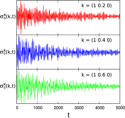
Figure 9: (Color online) Time evolution of $\sigma^{x}_{0}({\bf k},\,t)$ for different values of ${\bf k}$.

IV.2 Comparison with experiments

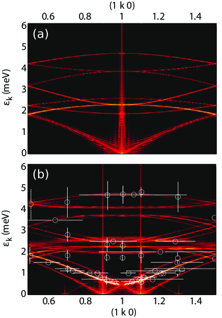
Figure 10: (Color online) (a) Spin wave spectrum of a Néel state with wavevector $\mathbf{q}=2\pi(0,0,1)$. This collinear order is the ground state of $\mathcal{H}$ with parameters $J=1.35$ meV, $K_{u}=0.21$ meV, $D=0$ meV, and $J_{3}=0.28$ meV. (b) Fitted spin wave spectrum to the neutron scattering measurement(white circles and rectangles)chung05 . The final set of parameters are $J=1.35$ meV, $K_{u}=0.21$ meV, $D=0.14$ meV, and $J_{3}=0.28$ meV. Note that adding DM interaction lifts the gap at $\mathbf{q}=2\pi(1,1,0)$ and splits each band into three. All the parameters are determined based on this fitting. Note that vertical peaks at the ordering wave vector $\mathbf{q}=2\pi(1,1\pm\delta,0)$ are numerical artifacts.

The magnon spectrum of $\mathrm{CdCr_{2}O_{4}}$ has been studied by Chung et al. using inelastic neutron scattering.chung05 Here we present our numerical calculations and compare the results with the experimental findings. The fact that the helical wavenumber $\delta\approx 0.09$ can be used to fix the ratio of the DM interaction to the exchange anisotropy $K_{u}$. On the other hand, values of $K_{u}$ and $K_{g}$ can be estimated by the magnon energies at the zone center, and we find that even tetragonal distortion does not play a significant role here. As for further-neighbor exchanges, ab initio calculations find a negligible $J_{2}$ and a quite large $J_{3}$ with antiferromagnetic sign. chern06 ; yaresko08 Using the following set of parameters: $J=1.46$ meV, $K_{u}=0.34$ meV, $K_{g}=0$ meV, $D=0.078$ meV, and $J_{3}=0.30$ meV, we obtained very good agreement with the experimentally measured spectrum, as shown in Fig. 10.

V Conclusion and Discussion

We have studied the spin-wave excitations in a special helical magnetic order on the pyrochlore lattice. This spiral structure characterized by a wavevector $\mathbf{Q}=2\pi(0,\delta,1)$ is observed in frustrated spinel CdCr₂O₄. Motivated by the experiments, we assumed that magnetic frustration is completely relieved by a tetragonal distortion which preserves the lattice translational symmetry. We have employed various analytical approaches and numerical methods to investigate the interplay of Dzyaloshinskii-Moriya interaction and further-neighbor couplings. Our spin-wave calculation with parameters inferred from structural data and ab initio calculations agrees well with the measured magnon spectrum. Combined with a systematic analysis of the helical structure, our study helps clarify the underlying mechanisms that stabilize the observed helical order and provides a quantitative description of the model Hamiltonian.

We have also shown that the continuum model of the spin spirals based on a gradient-expansion of the order parameter exhibits a continuous symmetry similar to that of smectic liquid crystals. A Goldstone mode with highly anisotropic dispersion results from the unique broken symmetry of the helical order. Although the emergent continuous symmetry is broken by the crystal fields effects at the microscopic level, our exact diagonalization on a large unit cell finds acoustic-like magnons which are reminiscent of the Goldstone mode discussed above.

Several recent experiments have established CdCr₂O₄ as the paradigmatic example of magnetic ordering induced by spin-lattice coupling in geometrically frustrated magnets. Although an overall tetragonal distortion with $a=b<c$ is observed below the ordering temperature, details of the lattice distortion remain to be clarified experimentally. The issue at hand is whether the distortion breaks the lattice inversion symmetry. As pointed out in a previous theoretical study, chern06 the broken parity plays an important role in stabilizing the observed helical order. This is because the lack of inversion symmetry endows the crystal structure with chirality, which is transferred to the magnetic order through relativistic spin-orbit interaction. Experimental evidence implying a broken parity in CdCr₂O₄ was recently reported in infrared absorption spectra. kant09 Our numerical calculation on spin-wave dispersions also indicates a predominantly tetragonal distortion which breaks the inversion symmetry, giving further support to the scenario that the helical magnetic order inherits its chirality from a lattice with broken parity.

Appendix A Spherical approximation

The matrices $J_{\mu\nu}(\mathbf{k})$ and $D^{\alpha\beta}_{\mu\nu}(\mathbf{k})$ in the spherical approximation (Eq. 8) are defined as follows:

$${\hat{J}}(\mathbf{k})=\left(\begin{array}[]{cccc}2J_{3}\left(\tilde{c}{}_{x\bar{y}}+\tilde{c}{}_{x\bar{z}}+\tilde{c}{}_{yz}\right)&(2J-K_{u})c_{yz}+3K_{u}s_{yz}&(2J-K_{u})c_{x\bar{z}}+3K_{u}s_{x\bar{z}}&2(J+K_{u})c_{x\bar{y}}\\ \\ (2J-K_{u})c_{yz}-3K_{u}s_{yz}&2J_{3}\left(\tilde{c}{}_{xy}+\tilde{c}{}_{xz}+\tilde{c}{}_{yz}\right)&2(J+K_{u})c_{xy}&(2J-K_{u})c_{xz}+3K_{u}s_{xz}\\ \\ (2J-K_{u})c_{x\bar{z}}-3K_{u}s_{x\bar{z}}&2(J+K_{u})c_{xy}&2J_{3}\left(\tilde{c}{}_{xy}+\tilde{c}{}_{x\bar{z}}+\tilde{c}{}_{y\bar{z}}\right)&(2J-K_{u})c_{y\bar{z}}+3K_{u}s_{y\bar{z}}\\ \\ 2(J+K_{u})c_{x\bar{y}}&(2J-K_{u})c_{xz}-3K_{u}s_{xz}&(2J-K_{u})c_{y\bar{z}}-3K_{u}s_{y\bar{z}}&2J_{3}\left(\tilde{c}{}_{x\bar{y}}+\tilde{c}{}_{y\bar{z}}+\tilde{c}{}_{xz}\right)\end{array}\right),\quad$$ (34)

$${\hat{D}}(\mathbf{k})=\sqrt{2}D\left(\begin{array}[]{cccccccccccc}0&0&0&0&-c_{yz}&-c_{yz}&0&c_{x\bar{z}}&0&0&0&c_{x\bar{y}}\\ 0&0&0&c_{yz}&0&0&-c_{x\bar{z}}&0&c_{x\bar{z}}&0&0&-c_{x\bar{y}}\\ 0&0&0&c_{yz}&0&0&0&-c_{x\bar{z}}&0&-c_{x\bar{y}}&c_{x\bar{y}}&0\\ 0&c_{yz}&c_{yz}&0&0&0&0&0&-c_{xy}&0&-c_{xz}&0\\ -c_{yz}&0&0&0&0&0&0&0&-c_{xy}&c_{xz}&0&c_{xz}\\ -c_{yz}&0&0&0&0&0&c_{xy}&c_{xy}&0&0&-c_{xz}&0\\ 0&-c_{x\bar{z}}&0&0&0&c_{xy}&0&0&0&0&c_{y\bar{z}}&-c_{y\bar{z}}\\ c_{x\bar{z}}&0&-c_{x\bar{z}}&0&0&c_{xy}&0&0&0&-c_{y\bar{z}}&0&0\\ 0&c_{x\bar{z}}&0&-c_{xy}&-c_{xy}&0&0&0&0&c_{y\bar{z}}&0&0\\ 0&0&-c_{x\bar{y}}&0&c_{xz}&0&0&-c_{y\bar{z}}&c_{y\bar{z}}&0&0&0\\ 0&0&c_{x\bar{y}}&-c_{xz}&0&-c_{xz}&c_{y\bar{z}}&0&0&0&0&0\\ c_{x\bar{y}}&-c_{x\bar{y}}&0&0&c_{xz}&0&-c_{y\bar{z}}&0&0&0&0&0\end{array}\right)$$ (47)

Note that here we use simplified notations defined as follows: $c_{\alpha\beta}=\cos(k_{\alpha}+k_{\beta})$, $c_{\alpha{\bar{\beta}}}=\cos(k_{\alpha}-k_{\beta})$, ${\tilde{c}}_{\alpha\beta}=\cos(2(k_{\alpha}+k_{\beta}))$, and $s_{\alpha\beta}=i\sin(k_{\alpha}+k_{\beta})$.

Appendix B Finite-difference method for integrating LLG equation

In this appendix, we discuss a finite difference scheme for numerical integration of the Landau-Lifshitz-Gilbert(LLG) equation by adopting the method introduced by Serpico et alserpico01 . The LLG equation can be written in the following form:

$$\frac{\partial{\bf S}_{i}}{\partial t}={\bf S}_{i}\times\left({\bf H}_{i}+\frac{\alpha_{G}}{S}\frac{\partial{\bf S}_{i}}{\partial t}\right),$$ (48)

Note that the effective exchange field ${\bf H}_{i}$ is defined in the Eq. (9).

Then the following approximations are applied on the midpoint between time step $n$ and $n+1$ :

$$\frac{\partial{\bf S}_{i}}{\partial t}(t_{n+1/2})=\frac{{\bf S}_{i}(t_{n+1})-{\bf S}_{i}(t_{n})}{\Delta t}+O(\Delta t^{2})$$ (49)

$${\bf S}_{i}(t_{n+1/2})=\frac{{\bf S}_{i}(t_{n+1})+{\bf S}_{i}(t_{n})}{2}+O(\Delta t^{2})$$ (50)

where $\Delta t=t_{n+1}-t_{n}$ and $t_{n+1/2}$ denotes midpoint between $t_{n}$ and $t_{n+1}$.

We now express ${\bf H}_{i}(t_{n+1/2})$ in terms of ${\bf H}_{i}(t_{n})$ and ${\bf H}_{i}(t_{n-1})$ by applying the midpoint approximation (50) twice :

$${\bf H}_{i}(t_{n+1/2})=\frac{3}{2}{\bf H}_{i}(t_{n})-\frac{1}{2}{\bf H}_{i}(t_{n-1})$$ (51)

By substituting Eq. (49),(50), and (51) into Eq. (48) we get:

$$\frac{{\bf S}_{i}(t_{n+1})-{\bf S}_{i}(t_{n})}{\Delta t}=\left[\frac{{\bf S}_{i}(t_{n+1})+{\bf S}_{i}(t_{n})}{2}\right]\times\left[\frac{3}{2}{\bf H}_{i}(t_{n})-\frac{1}{2}{\bf H}_{i}(t_{n-1})+\frac{\alpha_{G}}{S}\frac{{\bf S}_{i}(t_{n+1})-{\bf S}_{i}(t_{n})}{\Delta t}\right]$$ (52)

which yields the expression for ${\bf S}_{i}(t_{n+1})$ in terms of previous time step spin components ${\bf S}_{i}(t_{n})$ and ${\bf S}_{i}(t_{n-1})$:

$${\bf S}_{i}(t_{n+1})-{\bf S}_{i}(t_{n+1})\times\left[\left(\frac{3}{4}{\bf H}_{i}(t_{n})-\frac{1}{4}{\bf H}_{i}(t_{n-1})\right)\Delta t-\frac{\alpha}{S}{\bf S}_{i}(t_{n})\right]$$ (53)

$$={\bf S}_{i}(t_{n})+{\bf S}_{i}(t_{n})\times\left(\frac{3}{4}{\bf H}_{i}(t_{n})-\frac{1}{4}{\bf H}_{i}(t_{n-1})\right)\Delta t$$ (54)

Then the spin configuration ${\bf S}_{i}\left(t_{n+1}\right)$ is obtained by solving the matrix equation:

$${\bf S}_{i}(t_{n+1})={\bf B}_{i}(t_{n},t_{n-1})^{-1}{\bf A}_{i}\left(t_{n},t_{n-1}\right){\bf S}_{i}\left(t_{n}\right),$$ (55)

where ${\bf A}_{i}(t_{n},t_{n-1})$ and ${\bf B}_{i}\left(t_{n},t_{n-1}\right)$ are both $3\times 3$ matrix defined as follows :

$${\bf A}_{i}\left(t_{n},t_{n-1}\right)=\left(\begin{array}[]{ccc}1&-\mathcal{K}_{i}^{z}&\mathcal{K}_{i}^{y}\\ \mathcal{K}_{i}^{z}&1&-\mathcal{K}_{i}^{x}\\ -\mathcal{K}_{i}^{y}&\mathcal{K}_{i}^{x}&1\end{array}\right),$$ (56)

$${\bf B}_{i}(t_{n},t_{n-1})=\left(\begin{array}[]{ccc}1&\mathcal{F}_{i}^{z}&-\mathcal{F}_{i}^{y}\\ -\mathcal{F}_{i}^{z}&1&\mathcal{F}_{i}^{x}\\ \mathcal{F}_{i}^{y}&-\mathcal{F}_{i}^{x}&1\end{array}\right),$$ (57)

where $\hat{{\bf\mathcal{K}}}_{i}=\left[\frac{1}{4}{\bf H}_{i}(t_{n-1})-\frac{3}{4}{\bf H}_{i}(t_{n})\right]\Delta t$ and $\hat{{\bf\mathcal{F}}}_{i}=\hat{{\bf\mathcal{K}}}_{i}+\frac{\alpha_{G}}{S}{\bf S}_{i}(t_{n})$.

Appendix C Torques in the linearized LLG equation

The torques in the linearized time-dependent LLG equation (26) are calculated in this Appendix. First we choose the following parametrization for the local basis:

$$\begin{array}[]{l}{\bf\hat{e}}^{x}_{i}=\cos\theta_{i}\cos\phi_{i}{\bf\hat{a}}+\cos\theta_{i}\sin\phi_{i}{\bf\hat{b}}-\sin\theta_{i}{\bf\hat{c}}~{},\\ {\bf\hat{e}}^{y}_{i}=-\sin\phi_{i}{\bf\hat{a}}+\cos\phi_{i}{\bf\hat{b}}~{},\\ {\bf\hat{n}}_{i}=\sin\theta_{i}\cos\phi_{i}{\bf\hat{a}}+\sin\theta_{i}\sin\phi_{i}{\bf\hat{b}}+\cos\theta_{i}{\bf\hat{c}}~{},\end{array}$$ (61)

where $\theta_{i}$ and $\phi_{i}$ are polar and azimuthal angles that determine the orientation of spin at site $i$. Introducing the following notations for simplicity: $c_{i}=\cos\theta_{i}$, $s_{i}=\sin\theta_{i}$, ${\tilde{c}}_{i}=\cos\phi_{i}$, ${\tilde{s}}_{i}=\sin\phi_{i}$. the linearized torques projected onto the localized basis are:

$$\tau_{i}^{x} = \sum_{j}\Bigl{[}D_{ij}^{z}c_{j}{\tilde{c}}_{i-j}+\left(D_{ij}^{x}{\tilde{c}}_{i}+D_{ij}^{y}{\tilde{s}}_{i}\right)s_{j}+J_{ij}c_{j}{\tilde{s}}_{i-j}\Bigr{]}\,\sigma_{j}^{x}+\sum_{j}\Bigl{[}D_{ij}^{z}{\tilde{s}}_{i-j}-J_{ij}{\tilde{c}}_{i-j}\Bigr{]}\sigma_{j}^{y}$$ (62)

$$+ \sum_{j}\Bigl{[}\left(D_{ij}^{x}{\tilde{s}}_{i}-D_{ij}^{y}{\tilde{c}}_{i}\right)s_{i}c_{j}D_{ij}^{z}s_{i}s_{j}{\tilde{s}}_{i-j}+\left(D_{ij}^{y}{\tilde{c}}_{j}-D_{ij}^{x}{\tilde{s}}_{j}\right)\,c_{i}s_{j}+J_{ij}\left(c_{i}c_{j}+s_{i}s_{j}{\tilde{c}}_{i-j}\right)\Bigr{]}\sigma_{i}^{y},$$

$$\tau_{i}^{y} = \sum_{j}\Bigl{[}\left(D_{ij}^{y}{\tilde{c}}_{i}-D_{ij}^{x}{\tilde{s}}_{i}\right)s_{i}c_{j}+D_{ij}^{z}s_{i}s_{j}{\tilde{s}}_{i-j}+\left(D_{ij}^{x}{\tilde{s}}_{j}-D_{ij}^{y}{\tilde{c}}_{j}\right)c_{i}s_{j}-J_{ij}\left(c_{i}c_{j}+s_{i}s_{j}{\tilde{c}}_{i-j}\right)\Bigr{]}\sigma_{i}^{x}$$ (63)

$$+ \sum_{j}\Bigl{[}\left(D_{ij}^{y}{\tilde{c}}_{i}-D_{ij}^{x}{\tilde{s}}_{i}\right)c_{i}s_{j}-\left(D_{ij}^{y}s_{i}+D_{ij}^{z}c_{i}{\tilde{s}}_{i}\right)c_{j}{\tilde{c}}_{j}+\left(D_{ij}^{z}c_{i}{\tilde{c}}_{i}+D_{ij}^{x}s_{i}\right)c_{j}{\tilde{s}}_{j}+J_{ij}\left(c_{i}c_{j}{\tilde{c}}_{i-j}+s_{i}s_{j}\right)\Bigr{]}\,\sigma_{j}^{x}$$

$$+ \sum_{j}\Bigl{[}D_{ij}^{z}c_{i}{\tilde{c}}_{i-j}+\left(D_{ij}^{x}{\tilde{c}}_{j}+D_{ij}^{y}{\tilde{s}}_{j}\right)s_{i}+J_{ij}c_{i}{\tilde{s}}_{i-j}\Bigr{]}\sigma_{j}^{y}$$

References

- (1) R. Moessner and A. P. Ramirez, Physics Today 59 (2), 24 (2006).
- (2) R. Moessner and J. T. Chalker, Phys. Rev. Lett. 80, 2929 (1998); Phys. Rev. B 58, 12049 (1998).
- (3) J.-H. Chung, M. Matsuda, S.-H. Lee, K. Kakurai, H. Ueda, T. J. Sato, H. Takagi, K.-P. Hong, and S. Park, Phys. Rev. Lett. 95, 247204 (2005).
- (4) M. Matsuda, M. Takeda, M. Nakamura, K. Kakurai, A. Oosawa, E. Lelievre-Berna, J.-H. Chung, H. Ueda, H. Takagi, and S.-H. Lee, Phys. Rev. B 75, 104415 (2007).
- (5) R. Ballou, J. Deportes, R. Lemaire, Y. Nakamura, B. Ouladdiaf, J. Magn. Magn. Mater. 70, 129 (1987).
- (6) R. Cywinski, S. H. Kilcoyne, and C. A. Scott, J. Phys.: Condens. Matter 3, 6473 (1991).
- (7) S.-H. Lee, C. Broholm, T. H. Kim, W. Ratcliff, and S.-W. Cheong, Phys. Rev. Lett. 84, 3718 (2000).
- (8) H. Ueda, H. Mitamura, T. Goto, and Y. Ueda, Phys. Rev. B 73, 094415 (2006).
- (9) M. Matsuda, H. Ueda, A. Kikkawa, Y. Tanaka, K. Katsumata, Y. Narumi, T. Inami, Y. Ueda and S.-H. Lee, Nature Physics 3, 397 (2007).
- (10) T. Rudolf, Ch. Kant, F. Mayr, J. Hemberger, V. Tsurkan, and A. Loidl, New J. Phys. 9, 76 (2007).
- (11) S. Bhattacharjee, S. Zherlitsyn, O. Chiatti, A. Sytcheva, J. Wosnitza, R. Moessner, M. E. Zhitomirsky, P. Lemmens, V. Tsurkan, and A. Loidl, Phys. Rev. B 83, 184421 (2011).
- (12) S. Zherlitsyn, O. Chiatti, A. Sytcheva, J. Wosnitza, S. Bhattacharjee, R. Moessner, M. E. Zhitomirsky, P. Lemmens, V. Tsurkan and A. Loidl, J. Low Temp. Phys. 159, 134 (2010).
- (13) R. Valdes Aguilar, A. B. Sushkov, Y. J. Choi, S.-W. Cheong, and H. D. Drew, Phys. Rev. B 77, 092412 (2008).
- (14) Ch. Kant, J. Deisenhofer, T. Rudolf, F. Mayr, F. Schrettle, A. Loidl, V. Gnezdilov, D. Wulferding, P. Lemmens, and V. Tsurkan, Phys. Rev. B 80, 214417 (2009).
- (15) J.-H. Kim, M. Matsuda, H. Ueda, Y. Ueda, J.-H. Chung, S. Tsutsui, A. Q. R. Baron, and S.-H. Lee, J. Phys. Soc. Jpn. 80, 073603 (2011).
- (16) O. Tchernyshyov, R. Moessner, and S. L. Sondhi, Phys. Rev. Lett. 88, 067203 (2002); Phys. Rev. B 66, 064403 (2002).
- (17) O. Tchernyshyov and G.-W. Chern, pp. 269–291 in Introduction to Frustrated Magnetism, Springer Series in Solid-State Sciences, vol. 164, Eds. C. Lacroix, F. Mila, and P. Mendels (Springer, 2011).
- (18) A. Yoshimori, J. Phys. Soc. Jpn. 14, 807 (1959).
- (19) A. Adam, D. Billerey, C. Terrier, R. Mainard, L. P. Regnault, J. Rossat-Mignod, and P. Meriel, Solid State Commun. 35, 1 (1980).
- (20) J. N. Reimers, A. J. Berlinsky, and A.-C. Shi, Phys. Rev. B 43, 865 (1991).
- (21) G.-W. Chern, R. Moessner, and O. Tchernyshyov, Phys. Rev. B 78, 144418 (2008).
- (22) I. E. Dzyaloshinskii, J. Exp. Theor. Phys. 46, 1420 (1964).
- (23) T. Moriya, Phys. Rev. 120, 91 (1960).
- (24) M. Elhajal, B. Canals, R. Sunyer, and C. Lacroix, Phys. Rev. B 71, 094420 (2005).
- (25) B. Canals, M. Elhajal, and C. Lacroix, Phys. Rev. B 78, 214431 (2008).
- (26) G.-W. Chern, arXiv:1008.3038 (2010).
- (27) G.-W. Chern, C. J. Fennie, and O. Tchernyshyov. Phys. Rev. B. , 060405 (2006).
- (28) P. de Gennes and J. Prost, The Physics of Liquid Crystals (Clarendon Press, Oxford ,1993).
- (29) P. M. Chaikin and T. C. Lubensky, Principles of Condensed Matter Physics (Cambridge University Press, Cambridge UK, 1995).
- (30) L. Radzihovsky and T. C. Lubensky, Phys. Rev. E 83, 051701 (2011).
- (31) D. Belitz, T. R. Kirkpatrick, and A. Rosch, Phys. Rev. B 73, 054431 (2006).
- (32) M. Mochizuki, N. Furukawa, and N. Nagaosa. Phys. Rev. Lett. 104, 177206 (2010).
- (33) S. Kimura, M. Hagiwara, H. Ueda, Y. Narumi, K. Kindo, H. Yashiro, T. Kashiwagi, and H. Takagi, Phys. Rev. Lett. 97, 257202 (2006).
- (34) A. N. Yaresko, Phys. Rev. B 77, 115106 (2008).
- (35) C. Serpico, I. D. Mayergoyz, and G. Bertotti, J. Appl. Phys. 89, 11 (2001).