Reply to ”Comment on ’Detecting Non-Abelian Geometric Phases with Three-Level $\Lambda$ Atoms’ ”

Abstract

In this reply, we address the comment by Ericsson and Sjoqvist on our paper [Phys. Rev. A 84, 034103 (2011)]. We point out that the zero gauge field is not the evidence of trivial geometric phase for a non-Abelian SU(2) gauge field. Furthermore, the recalculation shows that the non-Abelian geometric phase we proposed in the three-level $\Lambda$ system is indeed experimentally detectable.

There are three points in the preceding comment Ericsson : (i) the sign in Eq.(7) in the original paperdu is wrong; (ii) non-Abelian geometrical phase(GP) of a large-detuned $\Lambda$ system ( $\sin\gamma\approx 0$ with $\gamma$ defined below) in the adiabatic approximation is trivial since the corresponding gauge field vanishes; (iii) the GP is still small in the general case with relatively large $\gamma$ and cannot be separated from the dynamical phase .

In this reply, we address the above comments. We agree with point (i). However, this mistake doesn’t influence the validity of the main result. We re-calculate the population difference induced by the geometric phase after correcting this sign error and find that the maximum population difference can still reach $20\%$. Such big population difference can be easily detected in a typical experiment.

We focus on the large-detuning case, where $\tan\gamma=(\sqrt{\Delta^{2}+\Omega^{2}}-\Delta)/\Omega\approx 0$ with $\Delta$ $(\Omega)$ the detuning (effective Rabi frequency). The large detuning can be easily realized through choosing proper parameters, i.e. $\Delta=1$ GHz and $\Omega=1$ MHz. As corrected in the commentEricsson , the gauge potentials in the large detuning case can be written as

$$A_{\theta} \approx i\cos{\varphi}\sigma_{y}+i\sin{\varphi}\sigma_{x},$$ (1)

$$A_{\varphi} \approx -i\sin^{2}{\theta}\sigma_{z}+i\sin{\theta}\cos{\theta}\cos{\varphi}\sigma_{x}$$

$$-i\sin{\theta}\cos{\theta}\sin{\varphi}\sigma_{y}.$$

Then we also agree that the corresponding gauge field $F_{\theta\varphi}$ must vanish.

One will think of such potentials like Eq.(1) and (2) may not bring any physical observable effects because of the vanished field strength. In the following we will illustrate with some examples that this granted judgement is wrong for non-Abelian gauge fields. The first example is about the vacuum solution in a Yang-Mills theory demonstrated in detail in Ref.Jackiw . Jackiw and Rebbi demonstrated thatJackiw , a type of gauge potentials in the Yang-Mills theory are gauge equivalent to the potential $A=0$ and thus the field strengths are vanished; however, the potentials should not be removed from the integrations over the field configurations by the gauge fixing procedure, and they argued that physical effects are associated with them. The second example we will address in detail is the well-known case that spin $1/2$ behavior in a time-dependent magnetic field $\mathbf{B}=(B_{x}(t),B_{y}(t),B_{z}(t))$Berry ; Bliokh . The interacting Hamiltonian is

$$H=\hbar\chi\mathbf{\sigma}\mathbf{B},$$ (3)

here $\sigma$ is the Pauli Matrixes and $\chi$ is the coupling constant. This Hamiltonian can be diagonalized through $H_{dg}=U^{-1}HU$ with the unitary matrix

$$U=\frac{1}{\sqrt{2B}}\left(\begin{array}[]{cc}\sqrt{B+B_{z}}&\sqrt{B-B_{z}}\\ \frac{B_{x}+iB_{y}}{\sqrt{B+B_{z}}}&-\frac{B_{x}+iB_{y}}{\sqrt{B-B_{z}}}\\ \end{array}\right),$$ (4)

here the corresponding eigenvalues are $E_{\pm}=\pm\hbar\chi B$, $B=|\mathbf{B}|$. For a pure gauge potential with the unitary matrix (4) as

$$\mathbf{A}(\mathbf{m})=iU^{-1}\frac{\partial U}{\partial\mathbf{m}},\mathbf{m}=(B_{x},B_{y},B_{z}),$$ (5)

the non-Abelian gauge field $\mathbf{F}$ is vanishing Bliokh . To recover the non-trivialness of such potential, one should choose a specific closed loop in this parameter space, i.e. , a loop with large enough $B$ to maintain the adiabatic approximation. In this case, the off-diagonal elements of $\mathbf{A}(\mathbf{m})$ are rejected and the adiabatic gauge potentials $\mathbf{A}^{(ad)}$ are given by

$$\mathbf{A}^{(ad)}=(\frac{B_{y}}{2B(B\pm B_{z})},-\frac{B_{x}}{2B(B\pm B_{z})},0),$$ (6)

where different signs correspond to two eigenvalue $E_{\pm}$. The corresponding field tensors are given by

$$F_{ij}^{(ad)}=\frac{\partial A_{j}^{(ad)}}{\partial m_{i}}-\frac{\partial A_{i}^{(ad)}}{\partial m_{j}}=\mp\varepsilon_{ijk}\frac{B_{k}}{2B^{3}},$$ (7)

$\varepsilon_{ijk}$ is the three order antisymmetric tensor. It can be seen that the closed path integral $\oint\mathbf{A}^{(ad)}d\mathbf{l}$ in these monopole field strength is just the case of Berry phase. This integral is non-zero and will bring physical observable effects. Furthermore, the integral should hold when we shrink the curve by decreasing $B$ linearly, then we return to the case of full matrix $\mathbf{A}(\mathbf{m})$. Therefore, $\oint\mathbf{A}(\mathbf{m})d\mathbf{l}$ also contains a flux and will bring physical observable effects. Namely, the non-vanishing $\oint\mathbf{A}(\mathbf{m})d\mathbf{l}$ is guaranteed by $\oint\mathbf{A}^{(ad)}d\mathbf{l}$ in the Abelian case. And hence, we show with the second exampe that the gauge potential with a zero gauge field will also have observable effects for its non-vanishing closed path integral in the non-Abelian case.

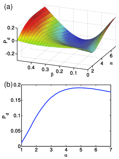
Figure 1: (color online).(a) The new result of population difference after two composed path with different orders. (b) The population difference $P_{d}$ versus parameter $\alpha$ when $\beta=0.5$. The parameters $\alpha$ and $\beta$ represent the relative amplitude and the time delay of Raman pulses in the stimulated Raman adiabatic transitions as the same in the origin paper du .

The situation of three-level $\Lambda$ atoms interacting with lasers is similar with the above analyzation. The unitary matrix diagonalize Hamiltonian (1) in du reads as

$$\Gamma=\left(\begin{array}[]{ccc}\cos{\theta}&-\sin{\theta}e^{-i\varphi}&0\\ \sin{\theta}\cos{\gamma}e^{i\varphi}&\cos{\theta}\cos{}\gamma&-\sin{\gamma}\\ \sin{\theta}\sin{\gamma}e^{i\varphi}&\cos{\theta}\sin{\gamma}&\cos{\gamma}\end{array}\right),$$ (8)

and $\gamma$ is given by $\tan{\gamma}=(\sqrt{\Delta^{2}+\Omega^{2}}-\Delta)/\Omega$. One can set large detuning $\Delta$ to achieve the non-Abelian geometric phase Eqs. (1,2). The corresponding gauge field is zero. To recover the non-trivialness of Eqs. (1,2), suitable $\Delta$ and $\Omega$ should be chose to reject the non-diagonal elements. Then we return to the Abelian case of which the gauge potential is $A^{\pm}_{\varphi}=\mp\sin^{2}{\theta}$ is observable Zhu . The non-zero closed path integral of $A^{\pm}_{\varphi}$ can be extended to the non-Abelian case just as the above analyzation. For example, we choose a closed loop of $\mathbf{A}=(A^{\prime}_{\theta},A^{\prime}_{\varphi})=i(A_{\theta},A_{\varphi})$ along $C$ with $\theta=\theta_{0}$, $\varphi\in[0,2\pi]$, and then the integral can be derived as

$$\oint\mathbf{A}d\mathbf{R}=\int_{0}^{2\pi}A^{\prime}_{\varphi}d\varphi=\pi(1-\cos 2\theta_{0})\sigma_{z}=\frac{1}{2}\Omega(C)\sigma_{z},$$ (9)

where $\Omega(C)$ is the solid angle spanned by $C$ which shows the geometric feature of the evolution. Clearly this integral is generally non-vanishing and then the corresponding geometric phase is non-trivial.

The result of a vanishing gauge field brings physical effects is counterintuitive. Indeed, this comes from the fact that the Stroke theorem in the non-Abelian case is not a direct generalization of the Abelian case. It has been realized that the surface integral in the non-Abelian case should depend on the gauge field $F_{\theta\varphi}$ as well as the gauge potential $\mathbf{A}$niu ; Barrett . Actually, the phase factor given as

$$U=\hat{P}\exp\left(i\oint\mathbf{A}\cdot d\mathbf{l}\right)$$ (10)

with $\hat{P}$ being the operator of chronological ordering, which is called the Wilson loopWilson , is of particular important for a non-Abelian field. This phase factor is transformed covariantly and may results in the observable physical effects even with zero field strengthBliokh ; Yang .

We re-calculate the possibly observed effects based on Eqs.(1) and (2). The new results are show in Fig.1, which should replace the results of Fig.2 in du . The procedure and parameters are the same with those in our original paperdu , but the gauge potentials are replaced with those in Eqs(1) and (2). We can find from Fig.1 that the maximum population difference can still reach almost $20\%$. Such big population difference can be easily detected in a typical experiment. Since $\gamma\approx 0.001$ for $\Gamma/\Delta=0.001$, we know that the effects induced by the dynamical phase could be neglected in the above calculation, as shown in the commentEricsson . Therefore, the population differences in Fig.1 are indeed induced by the non-Abelian gauge potential. Moreover, we directly calculate the Schrodinger equation $i\hbar\partial_{t}|\psi\rangle=H|\psi\rangle$ with the Hamiltonian given by Eq.(1) in Ref.Ericsson . We find that the results are the same with those in Fig.1 when the parameters are the same for the two different methods. It further confirms that the population difference is indeed caused by the non-vanished phase factor defined by the Wilson loop.

In summary, the main point that the authors used to defend in the comment is that the induced gauge field is zero and thus the GP is trivial. However, we have shown that this causality doesn’t hold for an SU(2) gauge field. Furthermore, we have shown that the non-Abelian GP in our proposal is non-trivial for its non-vanishing closed loop integral and can be detected through the induced significant population difference.

Acknowledge: The authors thank Z. B. Li, D. W. Zhang and S. L. Zhu for helpful discussions. This work was supported by the NSF of China(No. 11104085, No. 11125417, and No. 91121023 ), the SKPBR of China(No. 2011CB922104) and PCSIRT. Du was aslo supported by the SRFGS of SCNU.

References

- (1) M. Ericsson and E. Sjoqvist, comment (to be published in Phys. Rev. A).
- (2) Y. X. Du, Z. Y. Xue, X. D. Zhang and H. Yan, Phys. Rev. A 84, 034103 (2011).
- (3) R. Jackiw and C. Rebbi, Phys. Rev. Lett. 37, 172 (1976).
- (4) M. V. Berry, Proc. R. Soc. Lond. A 392, 45 (1984).
- (5) K. Yu. Bliokh and Yu. P. Bliokh, Anna. of Phys. 319, 13 (2005).
- (6) S. L. Zhu, H. Fu, C. J. Wu, S. C. Zhang and L. M. Duan, Phys. Rev. Lett. 97, 240401 (2006).
- (7) A. Bohm, A. Mostafazadeh, H. Koizumi, Q. Niu, J. Zwanziger, The Geometric Phase in Quantum Systems (Springer, New York, 2003).
- (8) T. Barrett and D. Grimes, Advanced Electromagnetism: Foundations, Theory, and application (World Scientific Publishing Co. Pte. Ltd., Singapore, 1995).
- (9) K.G. Wilson, Phys. Rev. D 10 (1974) 2445.
- (10) T. T. Wu and C. N. Yang, Phys. Rev. D 12, 3845 (1975); ibid. 12, 3843 (1975).