Toy model studies of tuning and typicality with an eye toward cosmology

Abstract

We investigate a number of simple toy models to explore interesting relationships between dynamics and typicality. We start with an infinite model that has been proposed as an illustration of how non-ergodic dynamics can produce interesting features that are suggestive for cosmological applications. We consider various attempts to define the infinite model more rigorously as a limit of a finite system. None of our attempts at such rigor were able to preserve the attractive properties. We hope our work will challenge others to find more successful toy models. The difficulty of finding such models suggests that connections between dynamics and typicality we hope for in cosmological theories such as eternal inflation may not be so easy to achieve.

I Introduction

Since the introduction of the idea of cosmic inflation Starobinsky (1980); Guth (1981); Linde (1982); Albrecht and Steinhardt (1982) many cosmologists have believed that a full theory of the cosmos should give us reason to think that the universe we observe is typical in some sense. This goal has proved difficult to achieve. The popular eternal inflation picture currently struggles under the measure problem as well as Page’s Born rule problem (probably the deeper of the two Albrecht and Phillips (2012)). The competing “de Sitter Equilibrium” picture Albrecht (2009, 2011) requires a controversial completion of the low energy effective theory, although it does avoid the measure and Born Rule problems and does exhibit typicality of the observed universe. The cyclic model, which is often offered as an alternative, has yet to be analyzed systematically regarding the typicality of our universe. For an overview of some of these issues see Albrecht (2012).

This paper seeks to take an incremental step in the study of these challenging issues by examining a number of toy models. The goal of these studies is to ask what can be said about “typicality” in some simple systems. We do not claim to offer grand insights into the cosmological problems here, as the toy models we consider are far simpler than realistic cosmologies. We only comment briefly about how certain features of our toy models might inform our thinking about cosmology. Still, we have found this investigation interesting and we believe this research can help us work toward more disciplined thinking about the cosmological case.

The starting point for our work is a toy model proposed by Guth Guth (2011) which is explicitly non-ergodic and has some very interesting features regarding typicality. We present this model in Section II. This toy model has traditionally been presented as a formally infinite system. We next study the same toy model where its infinite nature is more systematically constructed as a limit of a finite case (Sections III and IV). We show that the properties identified in the formally infinite case only appear if the limit is taken in a particular way, a way which requires constraints to be placed on the initial conditions. From that point of view the behavior originally identified appears to be less generic.

We next take up the question of whether a different toy model might exhibit significantly different properties (Section V). We investigate a second toy model with the phase space distorted or “bent” relative to that of the original model. The specific goal is to achieve an outcome different from that of the original model. Our analysis shows however that the bent model does not behave significantly differently from the original model, and if anything exhibits less of the desired behavior.

We present our interpretation and conclusions in Section VI. Our work raises concerns that the properties identified by Guth in his original toy model may not offer a path toward understanding typicality in cosmology, at least not without adding assumptions about initial conditions.

II Heuristic Description of the Infinite Case

Alan Guth has proposed a simple toy model that shows a natural tendency toward fine-tuning of parameters in an infinite phase space Guth (2011). The Hamiltonian for this model,

$$H_{PQ}=\tan^{-1}{(-PQ)},$$ (1)

is a canonical transformation of an upside-down simple harmonic oscillator (USHO), a particle moving in the potential

$$V(q)=-\frac{q^{2}}{2}.$$ (2)

Throughout this paper we use reduced coordinates which lead to the simple equation of motion

$$\ddot{q}=-\frac{dV}{dq}.$$ (3)

We consider the USHO model and we see that there are four quadrants in phase space (Fig. 1). The left quadrant corresponds to negative energy states where the particle moves right from $q=-\infty$, reaches its turning point, and returns to $-\infty$. The right quadrant corresponds to the mirror image of this where the particle starts at $q=+\infty$, reaches its turning point, and returns to $+\infty$. The top quadrant corresponds to the positive energy states where the particle starts at $q=-\infty$, continues over the top of the potential, and moves toward $+\infty$. The bottom quadrant is the mirror image of the top quadrant where the particle starts at $q=+\infty$, continues over the top of the potential, and moves toward $-\infty$.

Figure 1: Trajectories for the Upside-down Simple Harmonic Oscillator (USHO). The left and right quadrants correspond to bound states, whereas the top and bottom quadrants correspond to $E>0$. Squeezing toward the two asymptotes is an apparently universal behavior of this system.

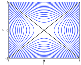
The key feature of this model is the flow of all trajectories toward the two diagonal asymptotes. This feature, known as “squeezing”, appears equivalently in each quadrant and for concreteness we zero in on the quarter of phase space that corresponds to bound states ($E<0$) where $q>0$. In this region, the trajectories are squeezed along the line $p=-q$ in the infinite past and along the line $p=q$ in the infinite future.

The special typicality property of this system can be stated as follows: Given any normalizable probability distribution, and some minimum amount of squeezing $S$ and small tolerance $\epsilon$ there will be some time, $T$, such that for every $t>T$, the probability of finding the system squeezed at least as much as $S$ will be greater than $1-\epsilon$. In other words, this system will spend an infinite amount of time in a squeezed state. We will discuss how to quantify squeezing in the next section, but the essence of this point can be readily seen by inspecting Fig. 1. Represent any normalizable probability distribution by the contour of your choice (say, the one that encloses $99\%$ of the probability). Then follow the evolution of that distribution by allowing each point on the contour to move along the trajectory on which it resides. Clearly the contour will get squeezed down to any set tolerance within a finite amount of time, and then spend the rest of eternity squeezing even further than that.

This is certainly not an ergodic system. If you inspect the system at a random time, it is highly unlikely to be found in just about any part of phase space, and is most likely to be found in a state arbitrarily squeezed against one of the asymptotes. The system is “naturally fine tuned”, in that a very special part of phase space (as measured by phase space area) is strongly preferred dynamically. One might hope that some behavior of this general sort might help us show how the finely tuned initial conditions of the big bang (or the apparently even more finely tuned initial conditions for an early inflationary phase) could be dynamically favored.

More realistic models might include a second phase of evolution during which the “attractor” region of phase space would be “on top of a hill” or dynamically interesting in some other way, or might distinguish between different past and future asymptotic behaviors. It is far from clear that the lessons we extract from the toy model considered here will survive if the complexity is increased in this way. We nonetheless hope that starting with the simplest toy models may be helpful in achieving a better understanding of these difficult problems. In particular, we treat squeezing against either asymptote as equivalent, since at the level of our simple models they are interchangable behaviors by a simple $t\rightarrow-t$ transformation.

Our discussion so far has dealt with infinities in a rather informal way. A more rigorous approach would be to consider this system as the limit of some finite system as it becomes very large. We do just that in the next section, and show that the limit must be taken in a special way to allow the interesting dynamical fine tuning to emerge.

III A Finite Case

We consider a simple way of making the upside-down simple harmonic oscillator finite by putting a sharp barrier at $q=a$, where $a$ is chosen based on how large we want our system. To achieve this we add a second term to the potential so that it becomes

$$V(q)=-\frac{q^{2}}{2}+\left(\frac{q}{a}\right)^{100}.$$ (4)

We call this the “USHO with barrier model” (USHOb). Once again, we focus on the $E<0$ and $q>0$ quadrant. Trajectories are shown in Fig.2. By increasing $a$, we increase the size of our system. Because the barrier is so sharp, most of the phase space to the left of the barrier is unchanged from the infinite case. But when the system approaches the barrier it rapidly reverses direction, sending the trajectory rapidly down the plot to connect with a trajectory with values of $p$ which are the opposite to the values before the barrier collision.

We consider the question: “Can the infinite case be thought of as the limit of this finite system as $a\rightarrow\infty$?” Because the trajectories in phase space are now closed, we can no longer say that a given trajectory will spend an infinite (or even necessarily an ever-increasing) amount of time in a squeezed state. In fact, there are some trajectories that will never enter a squeezed state. We now attempt to quantify these statements.

Figure 2: Trajectories for the USHOb system with the barrier placed at $a=10$. Introducing the barrier makes the system finite, creating a regulated version of the USHO system. (We show only one quadrant of phase space where $E<0$ and $q>0$).

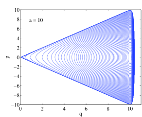
Begin by creating a patch of points in some region of phase space. This patch has a well-defined area in phase space and as it evolves in time along these trajectories, the phase space area will be conserved due to Liouville’s Theorem. This means that as it enters a region of larger squeezing, the patch is stretched along one direction and is squeezed along another. As an example, a circular patch starting in a region near $p=0$ for the infinite USHO model will become more stretched out along the direction parallel to $p=q$ and will become more squeezed along the direction perpendicular to $p=q$. The circular patch becomes more and more elliptical as time passes but the total area of this patch will remain constant. A problem with defining a squeeze parameter on this patch is that for a given starting position of the circular patch, the amount of squeezing will be dependent on the size of the patch. One way around this is to introduce a local definition for a squeeze parameter that will measure the amount of squeezing at a given point in phase space.

We choose to quantify squeezing in terms of the extent to which a given point is closer to one asymptote than the other. Even though “distance” has no physical meaning in phase space, the ratios of the distances to the two asymptotes are largely independent of the details of how those distances are computed, and to some extent even whether the geometry is assumed to be Euclidean. In any case, shifting our focus from the shape of the distribution to the proximity of the asymptotes allows us to construct a more useful squeeze parameter.

The (shortest, Euclidean) distance between a given point in phase space and the asymptote with slope $+1$ is given by $d_{+}=|{p-q}|/\sqrt{2}$, and the distance to the other asymptote is given by $d_{-}=|{p+q}|/\sqrt{2}$. We define our local squeeze parameter by

$$s\equiv\frac{d_{+}}{d_{-}}+\frac{d_{-}}{d_{+}}.$$ (5)

By this definition, the squeeze parameter is large whenever the phase space point is much closer to one asymptote than the other (regardless of which one is closer). Note that this is not at all a generic definition of squeezing, but instead makes use of the features of this particular model that cause the trajectories to be squeezed against particular asymptotes specific to the model.

Figure 3: The same phase space plot as Fig. 2, with lines of constant squeeze parameter $S$ shown superposed (dashed) on top of the USHOb trajectories. From top to bottom, $s=14,5,3,3,5,14$.

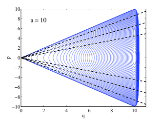
Figure 3 is equivalent to Fig. 2 with the addition of a few constant $s$ lines (solving Eqn. 5 for $p(q)$ with constant $s$ gives a pair of lines). The linear behavior of constant $s$ curves contrasted with the flow of the phase space trajectories strongly toward the asymptotes may suggest that our squeeze parameter is rather generously defined to favor large values. However, since this paper ultimately argues that squeezing is not as generically easy to achieve as one might have thought, making a generous definition of squeezing helps us make a more robust argument.

IV Trajectories

It is a simple task to lay down a set of trajectories for a given placement of the barrier. What fraction of time is spent above a given squeeze threshold by a given trajectory? By a given distribution of trajectories? What fraction of the area of phase space is above a given squeeze threshold? We discuss each of these questions in turn, in each case considering the limit as the squeeze threshold $a$ approaches infinity.

We start by selecting a large energy trajectory, since such trajectories will experience a lot of squeezing. The fraction of time a trajectory is squeezed is given by

$$f_{T_{i}}\equiv\frac{\Delta t_{\textrm{squeezed}}}{T_{\textrm{total}}}.$$ (6)

where $\Delta t_{\textrm{squeezed}}$ is the time spent above a given squeeze threshold and $T_{\textrm{total}}$ is the total time for the trajectory. Several squeeze thresholds are shown in Fig. 4, with $E=-0.001$, very close to the upper bound of $E=0$ for this quadrant. As we increase the size of the system by moving out the barrier, the fraction of time that this trajectory spends squeezed is continually increasing. This corresponds to the point of view described in Section II.

Figure 4: Fraction of time squeezed $f_{T_{i}}$ vs. barrier position $a$ for selected squeeze thresholds for an energy, $E=-0.001$, favorable to squeezing. The squeeze fraction increases as the barrier is moved to larger $a$ values.

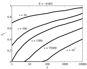
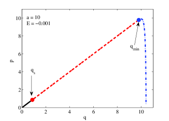
For an energy favorable to squeezing such as the one selected, we can derive this behavior analytically. Due to the symmetry across the $p=0$ axis, we only look at $p>0$, and we break the trajectory into three distinct portions, as shown in Fig. 5. The first goes from $p=0$ to $p=q_{s}$, the position where $s$ becomes greater than a given value. For sufficient squeezing, this point is independent of $a$. This portion of the trajectory is unsqueezed, and the time spent here ($\Delta t_{1}\equiv t_{s}-t_{0}$) is a constant, $c_{1}$, as the size of the system increases. (The linear appearance of the trajectory for small $q$ is due to its highly squeezed nature; the deviations from squeezing for $q<q_{s}$ are so small as not to be visible on the plot.) The second portion of this trajectory, $p=q_{s}$ to $p=q_{\textrm{min}}$ is squeezed, and extends to the point where $s$ again falls below the threshold value, which occurs at approximately the minimum of $V$ and is dependent on the value of $a$. Since the system is highly squeezed, the time $\Delta t_{2}=\int dq/p$ spent on this portion can be approximated by $\int dq/q$, and $\Delta t_{2}$ increases logarithmically with barrier position $a$. The third portion is once again unsqueezed, and runs from $p=q_{\textrm{min}}$ to the turning point of the potential. The time $\Delta t_{3}$ spent here is constant as well, which we call $c_{3}$. Referencing Eqn. (6), we see

$$f_{T_{i}}\approx\frac{\ln{\left({a}\right)}}{c_{1}+c_{3}+\ln{\left({a}\right)}},$$ (7)

which goes to $1-\epsilon$ with $\epsilon\equiv(c_{1}+c_{3})/\ln(a)$ for large values of $a$.

Figure 5: Regions used for our analytical treatment of fraction of time squeezed, with a threshold of $s=1500$, shown only for the half of the trajectory with $p>0$. The dashed line in the middle shows the squeezed portion of the trajectory.

Of course this is only one trajectory, and one more favorable to squeezing. Next we consider a discrete set of trajectories, covering the entire quarter of phase space, and average over them. However, the choice of trajectories affects the final results. To make an analogy to a ball rolling down a hill, each energy corresponds to the initial placement of the ball, and choosing more trajectories of larger energy means selecting more energies near the top of the hill. Since these trajectories become more squeezed than those of smaller energies, there should also be a bias to the fraction of time squeezed that is dependent on the set of trajectories we chose.

We choose a distribution of trajectories evenly spaced in energy up to $E=-10$. For a given distribution of trajectories such as this, we define the fraction of time this distribution spends squeezed as the simple average

$$f_{T}\equiv\frac{1}{N_{T}}\sum{f_{T_{i}}},$$ (8)

where $f_{T_{i}}$ is the fraction of time a given trajectory spends squeezed and $N_{T}$ is the number of trajectories. Once again, we arbitrarily choose several squeeze thresholds.

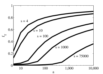
As shown in Fig. 6, as we increase the size of the system by moving out the barrier (while keeping the trajectory energies fixed), we again see that the fraction of time each trajectory spends squeezed continues to increase, and thus so does the average. As we move the barrier out there is an ever-increasing region of phase space that never reaches a fixed amount of squeezing (corresponding to the large central region of unsqueezed phase space clearly visible in Fig. 2 and illustrated in Fig. 7). But because we have fixed the trajectory energies to correspond to squeezing even for close barrier positions, the growing region of unsqueezed trajectories is not probed by our distribution. Thus, the limit we take here matches the intuition described in Sect. II, but does so at least in part because the distribution of trajectories is biased toward those that are more squeezed.

Figure 6: Fraction of time squeezed $f_{T}$ vs. $a$ for selected squeeze thresholds evaluated over an entire family of trajectories biased toward energies that favor squeezing.

Figure 7: Phase space trajectories illustrating how moving the barrier to larger $q$ values allows additional low energy trajectories that are less squeezed. The solid and dashed curves show trajectories for the same energy value, but the dashed curve has the barrier moved out to $a=20$ (vs $a=10$ for the solid curve). The dotted curve is an example of a trajectory with an energy that is forbidden when $a=10$, but is allowed when $a=20$ (or larger). Clearly the dotted curve is less squeezed than the others.

The previous distribution was chosen with some amount of arbitrariness. We could choose energies that fill phase space out to $E_{min}$, the minimum allowed energy for the given barrier position, and smooth out the bias towards higher energy trajectories by weighting energies that are closer together less than those that are farther apart. Numerically this corresponds to weighting each $f_{T_{i}}$ by $\Delta E_{\textrm{traj}}/\Delta E_{\textrm{Tot}}$, where

$$\Delta E_{\textrm{traj}}\equiv\lvert(E_{\textrm{next}}-E_{\textrm{previous}})\rvert/2$$ (9)

and $\Delta E_{\textrm{Tot}}$ is the total energy range of the family of trajectories from $0$ to $E_{\textrm{min}}$. Thus we have

$$f_{T_{E}}\equiv\sum{\frac{\Delta E_{\textrm{traj}}}{\Delta E_{\textrm{Tot}}}f_{T_{i}}}.$$ (10)

The results in this case are shown in Fig. 8a for several different squeeze thresholds. Now, as we move out the barrier to larger values, the fraction of time spent squeezed stays roughly constant (and a very small constant at that). Evaluating the squeeze fraction with this measure does not support the intuition presented in Sect. II.

We have therefore presented two different distributions for the initial trajectories that show different behaviors in the limit as the barrier is moved out. This illustrates that the possibility of having an increasing fraction of time squeezed is dependent on the selection of the initial distribution of trajectories.

(a)

(b)

Figure 8: Fraction of (a) time squeezed $f_{T_{E}}$ and (b) area squeezed $f_{A}$ vs. barrier position $a$ for selected squeeze thresholds. In (a) we use a distribution of trajectories of equally spaced energies, and moving out the barrier does not lead to larger squeeze fractions. As can be seen by comparing (b) with Fig. 3, the area fraction greater than some value is basically constant, modulo edge effects near the barrier.

We reiterate the message of Fig. 7: As the barrier is moved to larger $q$ values, the minimum of the potential goes down, opening up additional (lower) energy values that were simply not available to the system when the barrier was closer. The two distributions we have used so far treat these lower energy trajectories differently. The measure described by Eqn. 8 fixes the energy range to one that is allowed for a close barrier position, and simply excludes lower energies that become allowed as the barrier moves out. The measure described by Eqn. 10 brings in more energies as they become available (with a weighting that might be thought of as “equipartition” in energy). These differences are reflected in the different outcomes regarding the preference (or otherwise) for squeezing.

We now consider another measure that might be called “equipartition in phase space”: We simply measure a squeeze fraction weighted by phase space area. We lay down a grid on our region of phase space and find the average value for $s$ in each box. This means that the fraction of the area that is found above a given squeeze threshold is simply

$$f_{A}\equiv\frac{N_{s>s_{\textrm{thresh}}}A_{\textrm{box}}}{A_{\textrm{Tot}}},$$ (11)

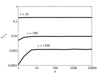
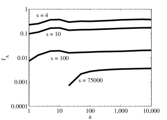
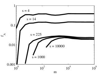
where $N$ is the number of boxes above a particular threshold, $A_{\textrm{box}}$ is the area of the individual boxes, and $A_{\textrm{Tot}}$ is the total area of phase space. For the selected squeeze thresholds, we see in Fig. 8b that roughly one percent of the area is squeezed for a threshold of $100$ even as the barrier for this system is moved to larger values of $a$. Larger thresholds exhibit even less area squeezed. This supports the conclusion that the amount of squeezing is constant as the size of the system increases. In fact, inspection of the locations of the constant $s$ lines in Fig. 3 makes it clear that a constant fraction of the phase space lies above any fixed squeeze value, modulo “edge effects” related to our discrete methodology, which are the source of the the non-constant aspects of the curves in Fig. 8b.

After analyzing the upside-down simple harmonic oscillator with a barrier, it appears that whether this finite system is overwhelmingly squeezed or not depends on how the question is asked. In particular, it appears that a bias or “prior” must be imposed on the trajectories as the limit of distant barriers is considered in order to realize the “universal squeezing” behavior discussed at an intuitive level in Sect. II. Thus if we consider the distant barrier limit of the finite system to be a more rigorous definition of the infinite case, the squeezing property is not really a universal property of the system at all. The heuristic discussion from Sect. II is only recovered when the limit is taken in a particular way, a way that imposes conditions on what “initial” states are considered.

V The Bent Phase Space Model

We have seen how trying to formulate the infinite USHO more rigorously as the limit of a finite system undermined the rather appealing intiuitive discussion we started with. But, perhaps this result is an artifact of that particular toy model.

With that question in mind, we choose to look at squeezing for another model that might show the intended results that increasing the size of the system more generically increases the squeeze fraction. Rather than making the system finite by placing an ordinary barrier at $q=a$, we choose a more complicated potential that makes the phase space finite, such as letting $V$ have both $p$- and $q$-dependence:

$$V(p,q)=-\frac{q^{2}}{2}+\left(\frac{1}{2(m-(q^{2}-p^{2}))}\right)^{50}+\left(\frac{1}{10(q^{2}-4p^{2})}\right)^{5}.$$ (12)

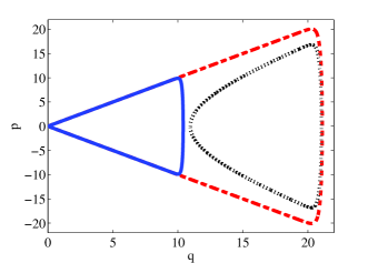
Changing the parameter $m$ corresponds to changing the size of the system. Fig. 9 shows trajectories for this model with $m=100$. We call this the “Bent Phase Space” (BPS) model. One other difference between this model and the USHO model is that in this model the lines of squeezing are now

$$p=\frac{q}{2};p=-\frac{q}{2}.$$ (13)

Since we have different asymptotic lines of squeezing we define a different squeeze parameter:

$$s_{B}\equiv\left\lvert\frac{2p+q}{2p-q}\right\rvert+\left\lvert\frac{2p-q}{2p+q}\right\rvert.$$ (14)

This model is chosen because the squeezing appears more pronounced, and because the barrier has a shape that appears to fit the lines of squeezing better than a simple barrier at $q=a$.

Figure 9: Trajectories for the Bent Phase Space (BPS) model with $m=100$ in the quadrant of phase space where $E<0$ and $q>0$. Constant $s_{B}$ curves are shown dashed, with values $s_{B}=70$, $7$ and $4$. The BPS model was chosen to be more favorable to squeezing.

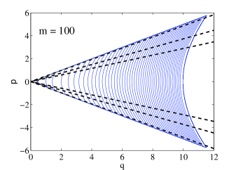
We are able to continue with the same analysis as for the USHOb and ask the same questions regarding how much time this model spends squeezed as well as how much of the phase space area is squeezed. Since the potential is now dependent on $p$, we no longer have $\dot{q}=p$ and instead have

$$\dot{q}=p\left(1-\frac{100}{2^{50}}\frac{1}{(m-(q^{2}-p^{2}))^{51}}+\frac{4}{10^{4}}\frac{1}{(q^{2}-4p^{2})^{6}}\right).$$ (15)

One can see that close to the asymptotes (given by Eqn. 13) the third term in $\dot{q}$ diverges. This means that a particle at a given energy will spend most of its time far away from the barrier and will pass close to asymptotes very quickly. It will also bounce off the barrier very quickly since $\dot{q}$ is large in that region. Fig. 10 shows this for a particular patch. One can also understand this effect intuitively by noting how the trajectories for the BPS model pack extremely closely together near the asymptotes. Liouville’s theorem then tells us that the patch must spread out extremely broadly in the direction along the trajectories.

Figure 10: Short squeeze duration in the BPS model: A patch started at $t=0$ (as shown in upper-left) will spend most of its time away from squeezed and barrier regions. As the squeezed region is approached small parts of the patch will move rapidly through to the other side. The time marked on each panel shows the different time scales involved. The patch is represented by a finite collection of points. A more continuous treatment would show the patch stretched very thinly along the trajectories followed by the isolated points.

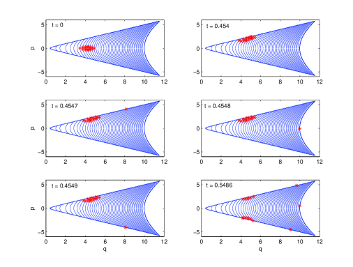
Once again the relevant concern is what happens as the size of the system grows large. The shape of the barrier seems to respect squeezing better than the USHOb model, yet a given particle moves through the squeezed region very quickly. To determine the net effect we choose a fixed squeeze threshold, $s_{B}$ and ask what happens to the squeeze fraction as we increase the parameter $m$.

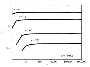
As before, we start by choosing a larger energy trajectory since we expect this will spend a large amount of time squeezed. Again, we arbitrarily choose several different squeeze thresholds. Using the same definition for $f_{T_{i}}$, we see in Fig. 11 that the fraction of time spent squeezed remains constant even as the size of the system increases. The expected effect due to the increase in size is canceled out by the increased speed of a particle in the squeezed regions. Very large squeeze values spend a negligible amount of time squeezed even for a favorable energy such as the one shown. Rather than explicitly considering the other “measures” defined for the USHOb model (specifically Eqns. 8 and 10), we see that since even an energy that is favorable toward squeezing shows a constant amount of time squeezed, any distribution of trajectories will display the same effects. The only difference between any of these time-based “measures” will be the exact value of the small fraction of time the distribution will spend squeezed.

Figure 11: The BPS model: Fraction of time squeezed $f_{T_{i}}$ vs. barrier position $m$ for selected squeeze thresholds for an energy, $E=-0.005$, favorable to squeezing. In contrast to Fig. 4 for the USHOb, the amount of squeezing does not increase with $m$, even for this very favorable case. The rapid motion of the BPS trajectories through the squeezed region is the reason that squeezing is not strongly favored in this model.

Finally, we look at the fraction of phase space area squeezed for this model (Fig. 12). The fraction of the area of phase space that is squeezed asymptotes to a constant value as well. This is clear from the fact that curves of constant squeezing in this model are once again straight lines like the USHOb model. Overall, it appears that rather than improving the USHOb model, the BPS model is even more unfavorable to squeezing.

Figure 12: The BPS model: Fraction of area squeezed $f_{A}$ vs. barrier position $m$ for selected squeeze thresholds. As can be seen from Fig 9 a constant area independent of $m$ is the natural large $m$ behavior.

VI Interpretation and Conclusions

VI.1 The Toy Models

In Section II we provided an intuitive analysis of the upside-down harmonic oscillator (USHO) which suggested that it had a highly universal squeezing behavior, independent of the initial conditions. Specifically, any initial region in phase space would in due course spend all of eternity in an arbitrarily squeezed state. As we discussed in the introduction, it has been hoped that this kind of behavior illustrates a phenomenon that could be put to good use in tackling difficult problems facing theoretical cosmology Guth (2011). However the USHO is an infinite system, and our heuristic discussion was quite loose in the way the infinity was handled. This paper has sought to study the phenomenon more rigorously by considering infinite models as limits of finite systems as their sizes are taken to infinity.

We have quantitatively analyzed the amount of squeezing for two different finite models. The first model was constructed by placing a barrier at $q=a$ for the USHO (creating the “USHOb” model). This model showed an increasing fraction of time squeezed as the size of the system increased for a specific chosen trajectory, as well as for a distribution of trajectories biased toward higher energies so as to favored squeezing. However, this model also showed squeeze fractions that were constant in time for a distribution that eliminated the higher energy bias. Thus for the USHOb model special assumptions or biases about the state of the system (i.e. the energies of the trajectories) are needed to recover the “eternal” squeezing behavior in the large system limit. If the limiting behavior of this system is taken to be a more rigorous description of the USHO model the attractive features of the USHO model do not look universal after all. Instead they appear to be closely tied to special assumptions about the state of the system.

The second model (the BPS model) had a more complicated behavior which superficially seemed more favorable to squeezing. However, when analyzed systematically this model too could not describe the hoped-for universal squeezing behavior. In fact, it’s behavior was even more problematic in that regard.

For each model, the squeeze values analyzed were chosen arbitrarily. The squeeze fractions were plotted versus the size of the system. However, another way of showing the same conclusions for each model was by plotting the squeeze fraction versus squeeze value and placing multiple system sizes on the same plot. Using this method, we are able to see trends in the squeeze values on a larger scale at the cost of being able to see the squeezing for a given value less clearly. These alternative methods of analysis support the conclusions previously stated in this paper.

Of course, all we have done is consider limits of two specific finite models. Perhaps there are other models that would offer a more positive outcome. And as we have discussed at the beginning, how the behavior of such toy models can be used to give insights into cosmological theories is a poorly developed subject. While we do not claim to have advanced that subject here, we conclude with some general comments about related issues in cosmology.

VI.2 Connection to Inflation

The project of calculating the probability of inflation taking place has generated considerable interest and controversy (for example Guth (2007); Hartle and Hawking (1983); *Gibbons:1986xk; *Hawking:1987bi; *Kachru:2003aw; *Gibbons:2006pa; *Linde:2007fr; *Carroll:2010aj; Schiffrin and Wald (2012)). People have tried a variety of approaches from classical phase space arguments to “wavefunctions of the universe” in quantum cosmology, to the dynamics of the string theory landscape, but so far there is no agreement as to the “right answer”. As emphasized in Albrecht and Sorbo (2004), the probability for inflation to start is an essential ingredient of any claim that inflation describes the most likely way of creating our observed universe. None the less, it is frequently hoped that in the limit where eternal inflation really lasts forever one can neglect any concerns about how low the probability may be of starting eternal inflation in the first place. Surely the infinite volume produced by eternal inflation will outweigh even an arbitrarily low probability for it to start, as long as that probability is nonzero. This would seem to allow us to make predictions despite the uncertainties surrounding the start of inflation.

More specifically, in Guth’s discussion of his toy model he argues that the squeezing (which he calls “tuning” in reference to the tuning of “initial” conditions required for realistic pocket universes) is completely generic Guth (2011) regardless of initial conditions. He then argues that the infinite phase space assumed in models of eternal inflation could lead to inflation and being generic through a similar sort of behavior. The intuitive picture of the USHO presented in Section II is just a restatement of this original argument by Guth. It appears to be a way that the dynamical behavior of a system can create a universal outcome regardless of initial conditions.

But to realize the hoped-for picture of eternal inflation one really needs to be much more rigorous than anyone has been so far. Schiffrin and Wald Schiffrin and Wald (2012) review some of these issues in a manner very much in the spirit of this paper. They identify not only the lack of equilibrium behavior emphasized and exploited by Guth Guth (2011), but also the importance of defining infinite systems rigorously, which is the focus of this paper. In the case of the toy model, we have attempted to improve the rigor by considering infinite systems as limiting cases of finite ones. This model can be thought of as a concrete realization of the limiting process discussed formally in section IV of Schiffrin and Wald (2012). Our approach should not be confused with various cutoffs used to regulate the infinities that come from the pocket universe counting problem. For one, imposing these cutoffs does not result in Hamiltonian systems, whereas all our models are Hamiltonian. Secondly, pocket universe formation is typically a quantum process which is clearly not present in our classical toy models. Also, as originally conceived in Guth (2011) the toy model was not intended to address the pocket universe counting problem. While we would be curious if the toy models offer an interesting perspective on that problem, we focus on Guth’s original topic of interest in this paper.

The failure of our finite toy models to realize the desired universal squeezing behavior in large size limit is an illustration of how things can go wrong. We add that the one case we know where eternal inflation has been considered as limit of a well-regulated finite system the outcome was opposite to the usual beliefs: The probability of starting inflation decreased sufficiently rapidly with increasing inflation duration that even when maximum impact of the increasing volume was assumed the probability of us living in an eternally inflating universe dropped to zero as the infinite limit was taken Albrecht and Sorbo (2004).

We have investigated simple toy models that we hoped would exhibit universal dynamics of the sort that would be nice to utilize in cosmological theories. Our attempts here to more rigorously treat earlier ideas along these lines yielded discouraging results, in that the desired universal behavior proved not so universal after all. We hope this work will stimulate other explorations which perhaps could yield toy models that do better. However, we suspect that the absence of successful models so far probably reflects a deeper problem with the idea that some sort of universal cosmological dynamics could explain the “typicality” of the universe we observe.