Counting Triangles in Massive Graphs with MapReduce

Abstract

Graphs and networks are used to model interactions in a variety of contexts. There is a growing need to quickly assess the characteristics of a graph in order to understand its underlying structure. Some of the most useful metrics are triangle-based and give a measure of the connectedness of mutual friends. This is often summarized in terms of clustering coefficients, which measure the likelihood that two neighbors of a node are themselves connected. Computing these measures exactly for large-scale networks is prohibitively expensive in both memory and time. However, a recent wedge sampling algorithm has proved successful in efficiently and accurately estimating clustering coefficients. In this paper, we describe how to implement this approach in MapReduce to deal with massive graphs. We show results on publicly-available networks, the largest of which is 132M nodes and 4.7B edges, as well as artificially generated networks (using the Graph500 benchmark), the largest of which has 240M nodes and 8.5B edges. We can estimate the clustering coefficient by degree bin (e.g., we use exponential binning) and the number of triangles per bin, as well as the global clustering coefficient and total number of triangles, in an average of 0.33 seconds per million edges plus overhead (approximately 225 seconds total for our configuration). The technique can also be used to study triangle statistics such as the ratio of the highest and lowest degree, and we highlight differences between social and non-social networks. To the best of our knowledge, these are the largest triangle-based graph computations published to date.

Keywords: triangle counting, clustering coefficient, triangle characteristics, large-scale networks, MapReduce

1 Introduction

Over the last decade, graphs have emerged as the standard for modeling interactions between entities in a wide variety of applications. Graphs are used to model infrastructure networks, the world wide web, computer traffic, molecular interactions, ecological systems, epidemics, co-authors, citations, and social interactions, among others. Understanding the frequency of small subgraphs has been an important aspect of graph analysis.

Despite the differences in the motivating applications, some topological structures have emerged to be important across all these domains. The most important such subgraph is the triangle (3-clique). Many networks, especially social networks, are known to have many triangles. This is thought to be because social interactions exhibit homophily (people befriend similar people) and transitivity (friends of friends become friends). The notion of clustering coefficient is inspired by this observation, and is the standard method of summarizing triangle counts [61, 40]. It is well known that some networks, especially social networks, have much higher clustering coefficients than random networks [38, 39, 41]. Triangle measures are important for understanding network structure and evolution [24, 48, 20, 60] and reproducing the degree-wise clustering coefficients of a network is important for generative models [22, 48, 51].

1.1 Our Contributions

For large graphs, computing triangle-based measures can be expensive. The standard approach is to find all wedges, i.e., paths of length 2, and check to see if they are closed, i.e., the edge that complete the triangle exists. Previous work presents a wedge-sampling approach for approximating clustering coefficients [50, 53]; this is in contrast to sampling single edges, which is a more obvious but less reliable technique. In [53], it is shown that the wedge-sampling approach is orders of magnitude faster than enumeration and is both faster and has less variance than edge-sampling techniques.

In this paper, we show that the wedge-sampling approach scales to massive networks using MapReduce, a framework well-suited to sampling. Previous distributed triangle counting algorithms have had to deal with problems of finding triangles where edges are stored on different processors and skewed degree distributions lead to load balancing issues [54, 3]. In contrast, our wedge sampling approach in MapReduce deals with these issues seamlessly and recommends sampling as a general technique for large graphs since it leads to fast serial algorithms as well as scalable parallel implementations. We describe our contributions in more detail as follows:

• We present a parallelization of our wedge-based sampling algorithm in the MapReduce framework. The premise of wedge sampling is to set up a distribution on the vertices (as potential wedge centers) and use that to sample the actual wedges. Designing a serial algorithm is easier, since the information to compute the distribution and then form the wedges is all local. In the MapReduce implementation, edges are distributed arbitrarily; therefore, it takes several passes to compute the necessary distribution, create the sample wedges, and finally check if they are closed.

• Additionally, we show that MapReduce enables computing multiple clustering coefficients for the same graph (e.g., binned by degree) for essentially the same cost as computing the single global clustering coefficient. Since the clustering coefficient generally varies with degree, it is helpful to see the profile versus a single value because these profiles are useful in graph characterization and modeling.

• We give extensive experimental results, on both real-world networks from the Laboratory for Web Algorithms as well as artificial networks created according to the Graph500 benchmark. We have multiple examples with more than a billion edges. To the best of our knowledge, these are the largest triangle computations to date.

• Results demonstrate the efficiency of our algorithm. For instance, we estimate the cost of computing clustering coefficients per (logarithmically) binned degree to be an average of 0.33 seconds per million edges plus overhead, which is approximately 225 seconds total for our 32-node Hadoop cluster. Hence, a graph with over 9B edges requires less than one hour of computation. Note that global clustering coefficient and total triangles are also computed.

• A straightforward implementation requires that the entire edge list be “shuffled” three times. We show how to greatly reduce the shuffle volume with some clever implementation strategies that are able to filter the edge list during the “map” phase. We discuss the implementation details and show comparisons of performance.

• A feature of wedge-based sampling is that the closed wedges are uniform random triangles. Hence, we also give experimental results characterizing triangles in terms of the their minimum and maximum degrees. Triangles from social networks tend to be somewhat assortative whereas triangles from other types of networks are not.

1.2 Related Work on Triangle Counting

Enumeration algorithms for finding triangles are either node- or edge-centric. Node-centric algorithms iterate over all nodes and, for each node $v$, check all pairs among the neighbors of $v$ for being connected. Edge-centric algorithms, on the other hand, go over all edges $(u,v)$ and seek common neighbors of $u$ and $v$. Chiba and Nishizeki [13] proposed a node-centric algorithm that orders the vertices by degree and processes each edge only once, by its lower-degree vertex. They showed that this algorithm runs in $O(m\alpha(G))$-time, where $m$ is the number of edges, and $\alpha(G)$ is the arboricity of the graph $G$ (arboricity is defined as the minimum number of forests into which its edges can be partitioned and can be considered as a measure of how dense the graph is). Schank and Wagner [50] used the same idea for their forward algorithm. Chu and Cheng studied an I/O efficient implementation of the same algorithm [15]. Latapy proved that the forward algorithm runs in $O(m^{3/2})$-time and proposed improvements that reduce the search space [31]. Latapy also showed that the runtime of this algorithm becomes $O(mn^{1/\alpha})$ for graphs with power-law degree distributions, where $\alpha$ is the power-law coefficient and $n$ is the number of vertices [31]. Arifuzzaman et al. [3] give a massively parallel algorithm for computing clustering coefficients. Pearce et al. [45] used triangle counting as an application to show the effectiveness external memory algorithms for massive graph analysis.

Enumeration algorithms however, can be expensive, due to the extremely large number of triangles (see e.g., Tab. 2), even for graphs even of moderate size (millions of vertices). Much theoretical work has been done on characterizing the hardness of exhausting triangle enumeration and finding weighted triangles [44, 62]. Eigenvalue/trace based methods adopted by Tsourakakis [58] and Avron [4] compute estimates of the total and per-degree number of triangles. However, the compute-intensive nature of eigenvalue computations (even just a few of the largest magnitude) makes these methods intractable on large graphs.

Most relevant to our work are sampling mechanisms. Tsourakakis et al. [56] initiated the sparsification methods, the most important of which is Doulion [59]. This method sparsifies the graph by retaining each edge with probability $p$; counts the triangles in the sparsified graph; and multiplies this count by $p^{-3}$ to predict the number of triangles in the original graph. One of the main benefits of Doulion is its ability to reduce large graphs to smaller ones that can be loaded into memory. However, the estimates can suffer from high variance [64]. Theoretical analyses of this algorithm (and its variants) have been the subject of various studies [29, 57, 42]. Another sampling approach has been proposed by Kolountzakis et al. [29], which involves both edge and triple-node sampling (a generalization of wedge-sampling). A MapReduce implementation of their method could potentially use many of the same techniques presented here. Alternative sampling mechanisms have been proposed for streaming and semi-streaming algorithms [5, 27, 7, 12]. Most recently, Jha et al. [25] showed how wedge-sampling can be performed when the graph is observed as a stream of edges and generalized their method for graphs with repeated edges [26]. An alternative approach and its parallelization were proposed by Tangwongsan et al. [55]. Many of these sampling procedures given above are by their very nature quite amenable to a MapReduce implementation.

The wedge-sampling approach used in this paper, first discussed by Schank and Wagner [49], is a sampling approach with the high accuracy and speed advantages of other sampling-based methods (like Doulion) but a hard bound on the variance. Previous work by a subset of the authors of this paper [53] presents a detailed empirical study of wedge sampling. It was also shown that wedge sampling can compute a variety of triangle-based metrics including degree-wise clustering coefficients and uniform randomly sampled triangles. This distinguishes wedge sampling from previous sampling methods that can only estimate the total number of triangles.

1.3 Related Work on MapReduce for Graph Analytics

MapReduce [17] is a conceptual programming model for processing massive data sets. The most popular implementation is the open-source Apache Hadoop [1] along with the Apache Hadoop Distributed File System (HDFS) [1], which we have used in our experiments. MapReduce assumes that the data is distributed across storage in roughly equal-sized blocks. The MapReduce paradigm divides a parallel program into two parts: a map step and a reduce step. During the map step, each block of data is assigned to a mapper which processes the data block to emit key-value pairs. The mappers run in parallel and are ideally local to the block of data being processed, minimizing communication overhead. In between the map and reduce steps, a parallel shuffle takes place in order to group all values for each key together. This step is hidden from the user and is extremely efficient. For every key, its values are grouped together and sent to a reducer, which processes the values for a single key and writes the result to file. All keys are processed in parallel.

MapReduce has been used for network and graph analysis in a variety of contexts. It is a natural choice, if for no other reason than the fact that it is widely deployed [34]. Pegasus [28] is a general library for large-scale graph processing; the largest graph they considered was 1.4M vertices and 6.6M edges and the PageRank analytic, but they did not report execution times. Lin and Schatz [36] propose some special techniques for graph algorithms such as PageRank that depend on matrix-vector products. MapReduce sampling-based techniques that reduce the overall graph size are discussed by Lattanzi et al. [32].

In terms of triangle counting and computing clustering coefficients, Cohen [16] considers several different analytics including triangle and rectangle enumeration. Plantenga [47] has studied subgraph isomorphism (i.e., finding small graph patterns such as triangles), including Cohen’s algorithm as a special case. (We use Plantenga’s implementation of Cohen’s Triangle enumeration algorithm for comparison in our subsequent numerical results.) For a non-triangle pattern, Plantenga’s SGI code ran on a 7.6B vertex graph with 107B undirected edges in 620 minutes on a 64-node Hadoop cluster. Wu et al. [63] have also studied triangle enumeration using MapReduce with running times of roughly 175 seconds on a graph with 1.6M nodes and 5.7M edges. Suri and Vassilvitskii [54] proposed a MapReduce implementation for exact per-node clustering coefficients. Most naive partitioning schemes do not give efficient parallelization because of high-degree vertices, and their result involves new partitioning methods to avoid this problem. We discuss how both [47] and [54] compare to our method in §5.3. SAHAD [66] has a Hadoop program that uses sampling techniques based on graph coloring to find subgraphs, but is limited to tree patterns. Ugander et al. [60] analyzed the Facebook graph with 721M nodes and 69B edges (representing friendships) on a 2,250 node Hadoop cluster. They sampled 500,000 nodes and computed the exact local clustering coefficient for each sampled node. They reported (binned) averages of the local clustering coefficients. We note that the binned local clustering coefficient is different than the binned global clustering coefficient which we calculate in this paper. Additionally, the approach of computing the exact local clustering coefficient for a set of sample nodes is non-trivial for general graphs since assembling the neighbors for high-degree nodes is extremely expensive. In the case of the Facebook graph, the maximum number of neighbors is only 5,000 (per Facebook policy); compare to our graphs which have nodes with over 1 million neighbors.

2 Background

2.1 Global Clustering Coefficient

Let $G=(V,E)$ be an undirected graph with $n=|V|$ nodes and $m=|E|$ undirected edges. We assume the vertices are indexed by $i=1,\dots,n$. Let $d_{i}$ denote the degree of vertex $i$; degree-zero vertices are ignored. A wedge is a length-2 path. Let $p_{i}$ denote the number of wedges centered at vertex $i$; i.e., $p_{i}={d_{i}\choose 2}=\frac{d_{i}(d_{i}-1)}{2}$. A wedge is closed if its endpoints are connected and open otherwise. The center of a wedge is the middle vertex. A triangle is a cycle with three vertices. A closed wedge forms a triangle; conversely, a triangle corresponds to three closed wedges. Let $t_{i}$ denote the number of triangles containing node $i$, which is equal to the number of closed wedges centered at node $i$. The node-level clustering coefficient (first used in [61]) is

$$c_{i}=\frac{t_{i}}{p_{i}}=\frac{\text{number of triangles incident to node $i$}}{\text{number of wedges centered at node $i$}}.$$

Thus, $c_{i}$ measures how tightly the neighbors of a vertex are connected amongst themselves.

We define $W$ to be the set of all wedges in $G$ and $p=|W|=\sum_{i}p_{i}$. We partition $W$ into two disjoint subsets as follows:

$$W_{0} =\Set{w\in W}{w\text{ open}},$$

$$W_{3} =\Set{w\in W}{w\text{ closed}}.$$

The subscript of 3 for the closed wedges indicates that each triangle creates 3 wedges in $W_{3}$. Let $t=\frac{1}{3}\sum_{i}t_{i}=\frac{1}{3}|W_{3}|$ denote the total number of triangles (since each triangle is counted thrice). The (global) clustering coefficient (also known as the transitivity) [40] of an undirected graph is given by

$$c=\frac{|W_{3}|}{|W|}=\frac{\sum t_{i}}{\sum p_{i}}=\frac{3t}{p}=\frac{3\times\text{total number of triangles}}{\text{total number of wedges}}.$$ (1)

At the global level, $c$ is an indicator of how tightly nodes of the graph are connected.

2.2 Binned Degree-wise Clustering Coefficient

In this paper, we will be using the binned degree-wise clustering coefficients, which measure how tightly the neighborhood of vertices of a specified degree group are connected. Let $D\subseteq\set{d_{i},d_{j},\dots}$ be a subset of degrees (recall that we ignore degree-zero nodes). We define $V_{D}=\set{i\in V}{d_{i}\in D}$ and $n_{D}=|V_{D}|$. In many cases, we are interested in a single degree, i.e., if $D=\set{d}$ then $V_{d}$ is the set of nodes of degree $d$ and $n_{d}$ is the number of nodes of degree $d$.

We define $W_{D}$ to be the set of all wedges centered at a node in $V_{D}$ and $p_{D}$ to be the total number of wedges centered at nodes in $V_{D}$, i.e., $p_{D}=|W_{D}|$. If $D=\Set{d}$, then $p_{d}=n_{d}{d\choose 2}$. We partition the set $W_{D}$ into four disjoint subsets as follows:

$$W_{D,0} =\Set{w\in W_{D}}{w\text{ open}},$$

$$W_{D,q} =\Set{w\in W_{D}}{w\text{ closed and has $q$ nodes in $V_{D}$}}\quad\text{for }q=1,2,3.$$

Define $p_{D,q}=|W_{D,q}|$ for $q=0,1,2,3$. Since $p_{D}=\sum_{q}p_{D,q}$, we can define binned degree-wise clustering coefficient, $c_{D}$, as the fraction of closed wedges in $W_{D}$; i.e.,

$$c_{D}=({p_{D,1}+p_{D,2}+p_{D,3}})/{p}.$$ (2)

The formula for triangles is more complex and given by

$$t_{D}=p_{D,1}+\frac{1}{2}\cdot p_{D,2}+\frac{1}{3}\cdot p_{D,3},$$

since for each triangle there is either one wedge in $W_{D,1}$, two wedges in $W_{D,2}$ or three wedges in $W_{D,3}$. Fig. 1 shows examples of these quantities when the bins are all singletons: $\set{1},\set{2},\set{3},\set{4}$.

Fig. 1: Example graph with various quantities highlighted.

3 Wedge Sampling for Triadic Measures

For a more detailed exposition of wedge sampling and empirical tests of its behavior, we refer the reader to [53]. For completeness, we review the relevant concepts and calculations here.

3.1 Hoeffding’s Inequality

The following result is a simple corollary of Hoeffding’s Inequality [23] (refer to Theorem 1.5 in [18]); the proof can be found in [53]. We say that $\varepsilon$ is the error and $(1-\delta)$ is the confidence.

Theorem 1.

Let $X_{1},X_{2},\ldots,X_{k}$ be independent random variables with $0\leq X_{i}\leq 1$ for all $i=1,\dots,k$. Define $\bar{X}=\frac{1}{k}\sum_{i=1}^{k}X_{i}$. Let $\mu=\mathbb{E}[\bar{X}]$. For any positive $\varepsilon,\delta$, setting $k\geq\lceil 0.5\varepsilon^{-2}\ln(2/\delta)\rceil$ yields

$${\rm Prob}\left\{|\bar{X}-\mu|\geq\varepsilon\right\}\leq\delta.$$

3.2 Binned Degree-wise Clustering Coefficients and Triangles

The strategy for computing the clustering coefficient per degree (or degree range) is similar to that described for the degree-wise clustering coefficient in [53].

Theorem 2 (Binned Degree-wise Clustering Coefficient).

For $\varepsilon,\delta>0$, set $k\geq\lceil 0.5\,\varepsilon^{-2}\ln(2/\delta)\rceil$. For $i=1,\dots,k$, choose wedge $w_{i}$ uniformly at random (with replacement) from $W_{D}$ and let $X_{i}$ be defined as

$$X_{i}=\begin{cases}1,&\text{if $w_{i}$ is closed},\\ 0,&\text{otherwise}.\end{cases}$$

Then

$${\rm Prob}\left\{|\hat{c}_{D}-c_{D}|\geq\varepsilon\right\}\leq\delta\quad\text{for}\quad\hat{c}_{D}=\frac{1}{k}\sum_{i=1}^{k}X_{i}.$$

Proof.

Observe that $c_{D}=\mathbb{E}[\bar{X}]$ since it is the probability that a random wedge in $W_{D}$ is closed. The proof follows immediately from Thm. 1. ∎

Choosing Uniform Random Wedges

We do not want to form all wedges explicitly. Instead, we implicitly generate random wedges. Observe that the number of wedges centered at vertex $i$ is exactly ${d_{i}\choose 2}$, and $p=\sum_{i}{d_{i}\choose 2}$. That leads to the following procedure. To select a random wedge, recall that $p_{D}=|W_{D}|$. Therefore, first choose vertex $i\in V_{D}$ with probability ${d_{i}\choose 2}/p_{D}$. Second, choose two distinct neighbors of vertex $i$ to form a random wedge. To set up this distribution, we need to compute the degree distribution. If $D=\Set{d}$ (a singleton), then all nodes in $V_{d}$ are equally probable. If $D=\set{0,+\infty}$, then the weight of vertex $i$ is ${d_{i}\choose 2}/p$.

Estimating the number of triangles is slightly more complicated since each closed wedge may have 1,2, or 3 vertices in $V_{D}$.

Theorem 3 (Degree-wise Triangle Count [53]).

Let the conditions of Thm. 2 hold. For each $w_{i}$, let $Y_{i}$ be defined as

$$Y_{i}=\begin{cases}1,&\text{if }w\in W_{D,1},\\ \frac{1}{2},&\text{if }w\in W_{D,2},\\ \frac{1}{3},&\text{if }w\in W_{D,3},\\ 0,&\text{if }w\in W_{D,0}\text{ (open) }.\\ \end{cases}$$

Then

$${\rm Prob}\left\{|\hat{t}_{D}-t_{D}|\geq\varepsilon\cdot p_{D}\right\}\leq\delta\quad\text{for}\quad\hat{t}=p_{D}\cdot\frac{1}{k}\sum_{i=1}^{k}Y_{i}.$$

Proof.

We claim $\mathbb{E}[Y]=t_{D}$. Suppose that $w$ is selected from $W_{D}$ uniformly at random. Observe that

$$\mathbb{E}[Y] ={\rm Prob}\left\{w\in W_{D,1}\right\}+\frac{{\rm Prob}\left\{w\in W_{D,2}\right\}}{2}+\frac{{\rm Prob}\left\{w\in W_{D,3}\right\}}{3}$$

$$=1\cdot\frac{p_{D,1}}{p_{D}}+\frac{1}{2}\cdot\frac{p_{D,2}}{p_{D}}+\frac{1}{3}\cdot\frac{p_{D,3}}{p_{D}}$$

$$=t_{D}/p_{D},$$

per (2.2). Hence, from Thm. 1 we have

$${\rm Prob}\left\{|\hat{t}_{D}/p_{D}-t_{D}/p_{D}|\geq\varepsilon\right\}\leq\delta,$$

and the theorem follows by multiplying the inequality by $p_{D}$. ∎

3.3 Computing a Random Sample of the Triangles

In addition to knowing the number of triangles in a graph, it may also be interesting to consider the properties of those triangles. For instance, Durak et al. [19] consider the differences in node degrees in a triangle.

It turns out that the closed wedges discovered during the wedge sampling procedure are triangles sampled uniformly (with replacements). Hence, we can study these randomly sampled triangles to estimate the overall characteristics of triangles in the graph.

Theorem 4.

Let $W_{s}$ be a random sample of the wedges of a graph $G$, and let $T_{s}\subseteq W_{s}$ triangles that are formed by the closed wedges in $W_{s}$. Then each triangle in $T_{s}$ is a uniform random sample from the triangles of $G$.

Proof.

The proof depends on observing that a triangle being chosen depends only on one of its 3 wedges being chosen. Since the wedge sample is uniformly random, each triangle is equally likely to be picked, and there is no dependency between any pair of triangles, which implies a uniform sample. ∎

3.4 Practical Performance of Wedge Sampling

Earlier work by a subset of the authors [53] provides a thorough study on how the techniques described above perform in practice. As expected, tremendous improvements are achieved in runtimes compared to full enumeration, especially for large graphs, since the number of samples is independent of graph size. Specifically, we see speed-ups of more than 1000X with errors in the clustering coefficient of less than 0.002. Additionally, in comparison to the Doulion method (an edge-sampling technique) we obtain speed-ups of 5X or more while obtaining the same accuracy. The ability to adapt our wedge-sampling method to computing binned degree-wise clustering coefficients and triangle sampling are also benefits in comparison to edge-based sampling.

Our goal in this work is to implement the wedge sampling approach within the MapReduce framework and provide evidence that it can scale to much larger problems.

4 MapReduce Implementation

4.1 Overview

We now present a MapReduce algorithm for estimating the clustering coefficients and number of triangles in a graph. For details on MapReduce, we refer the reader to Lin and Dyer [35]; we have emulated their style in our algorithm presentations. We use the open-source Hadoop implementation of MapReduce, and the Hadoop Distributed File System (HDFS) for storing data. Each MapReduce job takes one or more distributed files as input. These files are automatically stored as splits (also known sometimes as blocks), and one mapper is launched per split. The mappers produce key-value pairs. All values with the same key are sent to the same reducer. The number of reducers is specified by the user. Each MapReduce job produces a single HDFS output file. A MapReduce job accepts configuration parameters, which are passed along as data to the mapper and reducer functions; we discuss these in more detail in the sections that follow. The set of MapReduce jobs in our algorithm is coordinated by a Hadoop Java program running on a single client node.

In our code, we assume the nodes are binned by degree as discussed in §4.2. Computation of the global clustering coefficient is a special case which can be computed by either looking only at a single bin containing all degrees or using a weighted average of the binned clustering coefficients (see §4.6.2).

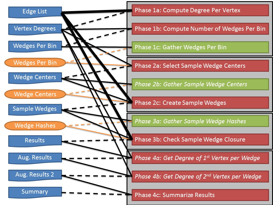
Our input is an undirected edge list where the node identifiers are 64-bit integers; we assume no duplicates or self-edges and no particular ordering. We divide our MapReduce algorithm into three major phases plus post-processing, as presented in Fig. 2. Each major phase makes a complete pass through the edge list. The first phase sets up the distribution on wedges. The second phase creates the sample wedges. Finally, the third phase checks whether or not the sample wedges are closed. In all three phases, we have strategies to reduce the data volume in the shuffle phase (between the map and reduce), discussed in detail in the sections that follow.

Fig. 2: Algorithm overview for estimating clustering coefficients and counting triangles, both binned by degree. Red boxes indicate a MapReduce job, while green represents a serial operation on the client node. Blue boxes indicate data files. The edge list is provided by the user; all other data files are produced by the method. Orange boxes indicate data that is passed as a “configuration parameter” to all mappers. Solid lines indicate consumption of data. Dotted lines indicate creation of data.

4.2 Binning

We define degree bins in a parameterized way as follows. Let $\tau$ be the number of singleton bins, and let $\omega>1$ be the rate of growth on the bin sizes. The first $\tau$ bins are singletons containing degrees $1,2,\cdots,\tau$ respectively. The remaining bins grow exponentially in size.

We describe the lowest degree of bin $k$ as

$$\textsc{BinLoDeg}(k)=\begin{cases}k,&\text{if }k\leq\tau,\\ \lceil(\omega^{(k-\tau)}-1)/(\omega-1)\rceil+\tau,&\text{otherwise.}\end{cases}$$ (3)

The highest degree for bin $k$ is just one less than the lowest degree of bin $k+1$. For a given degree $d$, we can easily look up its bin as

$$\textsc{BinId}(d)=\begin{cases}d,&\text{if }d\leq\tau,\\ \lfloor\log(1+(\omega-1)(d-\tau))/\log(\omega)\rfloor+\tau,&\text{otherwise.}\end{cases}$$ (4)

In our implementation, $\tau$ and $\omega$ are communicated to each MapReduce job as configuration parameters.

For $\tau=2$ and $\omega=2$, the bins are $\set{1}$, $\set{2}$, $\set{3,4}$, $\set{5,6,7,8}$, $\set{9,\dots,16}$, $\set{17,\dots,32}$, and so on. Note that the bin $\set{1}$ cannot have any wedges, so we just ignore it. Let $\bar{d}$ be an upper bound on the highest degree for a given graph. Then choosing $\tau=1$ and $\omega=\bar{d}$ yields bins $\set{1},\set{2,\dots,\bar{d}}$. In other words, we have a single bin containing all vertices (excepting degree-1 vertices). On the other hand, choosing $\tau=\bar{d}$ yields $\set{1},\set{2},\dots,\set{\bar{d}}$. Here, every bin is a singleton.

We are not constrained to equation (4) for computing the bins; we can use any procedure such that each degree is assigned to a single bin. Likewise, (3) is optional and used to reduce the shuffle volume in Phase 2c.

4.3 Phase 1: Compute Degree-based Statistics

4.3.1 Phase 1a: Compute Degree per Vertex

Phase 1a is a straightforward MapReduce task—computing the degree of each vertex. The Map and Reduce functions are described in Alg. 1. The input is the edge list file; each entry is a pair of vertex IDs $(v,w)$ that define an edge. The Map function is called for each edge $(v,w)$ and emits two key-value pairs keyed to the vertex IDs and having a value of 1. The Reduce function gathers all the values for each vertex and sums them to determine the degree. The final output to HDFS is a vertex degree file; each entry is of the form $(v,d)$ where $v$ is a vertex ID and $d$ is its degree.

Algorithm 1 Compute Degree per Vertex (Phase 1a)

method Map($v,w$) $\triangleright$ Input is edge list file

    Emit$(v,1)$

    Emit$(w,1)$ $\triangleright$ Emit both for an undirected graph

method Reduce($v,\set{x_{1},x_{2},\ldots}$)

    $d\leftarrow\textsc{Sum}(\set{x_{1},x_{2},\ldots})$ $\triangleright$ Compute degree

    Emit$(v,d)$ $\triangleright$ Output is vertex degree file

Alg. 1 shows a simple version of the code. To make the code more efficient, we collect local counts within each mapper (using a Java Map container) and emit the totals. This technique is called an in-memory combiner [36]. We found the in-memory combiner to reduce shuffle volume more than employing the reducer as a combiner.

4.3.2 Phase 1b: Compute Number of Wedges per Bin

Phase 1b works with the output of Phase 1a (vertex degree file) to compute the number of wedges per bin. The Map and Reduce functions for Phase 1b are presented in Alg. 2. The input is the list of degrees per vertex. The Map function is called for each vertex (with its associated degree) and emits the number of wedges for that vertex, keyed to the appropriate bin. The Reduce function simply combines the results for each bin. The final output is a wedges per bin file; each entry is of the form $(b,n_{b},p_{b})$ where $b$ is the bin ID, $n_{b}$ is the number of vertices in the bin, and $p_{b}$ is the number of wedges in the bin.

Algorithm 2 Compute Number of Wedges per Bin (Phase 1b)

parameters: $\tau,\omega$ $\triangleright$ Binning parameters

method Map($v,d$) $\triangleright$ Input is vertex degree file

    $b\leftarrow\textsc{BinId}(d,\tau,\omega)$ $\triangleright$ Compute bin ID

    $n\leftarrow 1$ $\triangleright$ Number of vertices

    $p\leftarrow d\cdot(d-1)/2$ $\triangleright$ Number of wedges

    Emit$(b,(n,p))$

method Reduce($b,\set{(n_{1},p_{1}),(n_{2},p_{2}),\ldots}$) $\triangleright$ One reduce function per bin

    $n\leftarrow\textsc{Sum}(\set{n_{1},n_{2},\ldots})$ $\triangleright$ Number of vertices in bin

    $p\leftarrow\textsc{Sum}(\set{p_{1},p_{2},\ldots})$ $\triangleright$ Number of wedges in bin

    Emit$(b,n,p)$ $\triangleright$ Output is wedges per bin file

Once again, we have shown a simple version of the algorithm in Alg. 2. To make the code more efficient, we collect local counts within each mapper (using a Java Map container) and emit the totals.

For the case of a single bin, strictly speaking, Phase 1b is unnecessary. Instead, we could have used a Hadoop global counter to tally the total wedges in the reduce step of Phase 1a.

4.3.3 Phase 1c: Gather Wedges per Bin

From the wedges per bin file (output of Phase 1b), we create a wedges per bin object, which acts as a function $\theta$ such that $\theta(b)$ is the number of wedges in bin $b$. The work is performed entirely in our main program running on the client node. It reads Phase 1b output from HDFS, stores wedges per bin values in a Java Map container, and launches the next MapReduce job (Phase 2a), sending the serialized container as a configuration parameter.

4.4 Phase 2: Select Wedge Samples

4.4.1 Phase 2a: Select Sample Wedge Centers

The input to Phase 2a is the vertex degree file along with the wedges per bin object, which is passed as a configuration parameter. Phase 2a calculates the number of sample wedges centered at each vertex. The Map function is shown in Alg. 3. The Map function is called for each (vertex ID, degree) pair. From this, we can calculate the expected number of wedges that would be sampled from the vertex for a uniform random sample, $q^{*}$. This number is unlikely to be integral. Rounding up would produce far too many wedges. Instead, we use probabilistic rounding. For instance, if $q^{*}=0.1$, then there is a 10% change of producing $q=1$ wedges and a 90% chance of producing no wedges, $q=0$. We are only off by at most one, so if $q^{*}=1.1$, then there is a 10% change of producing $q=2$ wedges and a 90% chance of producing $q=1$ wedge. Hence, the expected number of wedges for this vertex is exactly $q^{*}$. Only vertices with at least one sample wedge are emitted. The final output is a wedge centers file; each entry is of the form $(v,d,q,p)$ where $v$ is the vertex ID, $d$ is the vertex degree, $q$ is the number of sample wedges centered at that vertex, and $p$ is the total number of wedges in the bin containing $v$. The Reduce function is just the identity map and is not shown.

Algorithm 3 Determine number of samples per vertex (Phase 2a)

parameter: $k$ $\triangleright$ Desired number of samples per bin

parameter: $\theta$ $\triangleright$ Represents wedges per bin object

method Map($v,d$) $\triangleright$ Input is vertex degree file

    $b\leftarrow\textsc{BinId}(d)$ $\triangleright$ Compute bin ID

    $p\leftarrow\theta(b)$ $\triangleright$ Total number of wedges in bin containing $v$

    $q^{*}\leftarrow(d\cdot(d-1)/2)\cdot k/p$ $\triangleright$ Ideal number of samples, likely noninteger

    $x\leftarrow\textsc{rand }([0,1])$ $\triangleright$ Uniform random number in $[0,1]$

    $q\leftarrow\set{x\geq(q^{*}-\lfloor q^{*}\rfloor)}\text{ ? }\lceil q^{*}\rceil:\lfloor q^{*}\rfloor$ $\triangleright$ Number of sample wedges centered at $v$

    if $q\geq 1$ then $\triangleright$ Skip vertices with no samples

         Emit$(v,d,q,p)$ $\triangleright$ Output is wedge centers file

    end if

4.4.2 Phase 2b: Gather Sample Wedge Centers

Phase 2b is an optional step that generates a Java Map of wedge centers and their bin IDs based on the output of Phase 2a (wedge centers file). We represent this object as a function $\gamma$ such that

$$\gamma(v)=\begin{cases}0&\text{if Phase 2b is skipped},\\ 1&\text{if $v$ is not a wedge center},\\ b\geq 2&\text{if $v$ is a wedge center, in which case $b$ is the bin ID}.\end{cases}$$

This wedge centers object has one value for every vertex appearing in a wedge center. It is serialized and passed as a configuration parameter to Phase 2c, where it is used to filter the edges that are emitted by the Map function.

Note that Hadoop imposes a limit on the size of the configuration parameters (5MB by default). If the number of wedge centers is too large (a few hundred thousand samples will exceed 5MB), then other options must be explored. One alternative is to pass the container to the Map tasks using the Hadoop distributed cache; however, we have not implemented this idea.

Phase 2b is optional, and can be skipped if there are too many wedge centers. We demonstrate the benefits of this step in §5.

4.4.3 Phase 2c: Create Sample Wedges

In Phase 2c, the goal is to take each sample wedge center (from the wedge center file), collect its neighbors (from the edge list file), and create a set of sample wedges. We merge each vertex and its neighbors at the reduce phase. If it exists, the optional wedge center object is used to filter the edges that are shuffled, ignoring all edges that are not adjacent to a sampled wedge center. The algorithm is shown in Alg. 4. For clarity, we give a separate Map function for each input type. In the actual implementation, we have to determine the input type on the fly, because both input files are of Hadoop type Text. For input from the wedge centers file, the Map function simply passes along its degree and sample wedge count (i.e., the number of wedges to be sampled from the vertex).

For input from the edge list file, the Map function checks to see if the edge is adjacent to a wedge center. If so, it is passed based on the outcome of a random coin flip. The aim of the Reduce phase is to generate random wedges centered at a vertex (say $v$). The most naïve Map implementation would forward all edges incident to $v$, so that wedges can be selected from them. A major problem with this is that if the number of samples $k$ is much less than the degree of $v$, most of the communication is unnecessary. For example, the highest degree vertices of a social network graph might link to millions of edges, but $k$ is in the tens of thousands or less; therefore, most of the incident edges will not participate in sampled wedges centered at these vertices. We have a probabilistic fix to address this situation.

We do not have the vertex degree readily available, but we do know its bin and therefore a lower bound on its degree. Consider a vertex $v$ of degree greater than $d_{\min}$, where $2k\leq d_{\min}/2$. We send just some of the incident edges to $v$, with independent probability $\phi=4k/d_{\min}\leq 1$. Then the expected number of edges to send is $4k(d_{v}/d_{\min})$. Note that this expectation is at least $4k$. Getting less than $2k$ edges is potentially disastrous, but the probability of this is minuscule. By a multiplicative Chernoff bound (given below), the probability of such an event is $\exp(-k/8)$. For $k=1000$ (a tiny sample size), the probability is less than $10^{-55}$.

Theorem 5 (Multiplicative Chernoff Bound [18]).

Let $X=\sum_{i\leq r}X_{i}$, where each $X_{i}$ is independently distributed in $[0,1]$. Then

$${\rm Prob}\left\{X\leq(1-\delta)\mathbb{E}[X]\right\}\leq\exp(-\delta^{2}\mathbb{E}[X]/2).$$

If $d_{v}$ is not too far from $d_{\min}$, then the expectation $4k(d_{v}/d_{\min})$ is potentially much smaller than $d_{v}$. Hence, we get the desired number of random edges without sending too many.

Even with this improvement, the data passed forward may be too large to fit into the reducer’s memory. We use a feature of Hadoop called secondary sort to ensure that the data arrives pre-sorted. Note that the key used for passing along the vertex information is $v\mathtt{:}0$ and the key for the edges is of the form $v\mathtt{:}y$, where $y$ is a random positive integer. This data is all mapped to the key $v$, but the values following the colon control the sort of the values associated with $v$. The secondary key of zero ensures that the degree and wedge count data are first. The secondary keys for edges ($y$) ensure that the adjacent edges are randomly sorted; otherwise, Hadoop would present the edges in their order of arrival, which could bias the selection.

Algorithm 4 Create Sample Wedges (Phase 2c)

parameters: $\tau,\omega$ $\triangleright$ Binning parameters

parameter: $k$ $\triangleright$ Desired number of samples per bin

parameter: $\gamma$ $\triangleright$ Represents wedge centers object

method Map($v,d,q,p$) $\triangleright$ Input is wedge centers file

    Emit$(v\mathtt{:}0,(d,q,p))$ $\triangleright$ Note secondary sort key

method Map($v,w$) $\triangleright$ Input is edge list file

    EdgeHelper($v,w$)

    EdgeHelper($w,v$)

method EdgeHelper($v,w$)

    $b\leftarrow\gamma(v)$ $\triangleright$ Extract bin ID

    if $b=0$ then $\triangleright$ Phase 2b was skipped

         $\phi\leftarrow 1$ $\triangleright$ Always emit the edge

    else if $b=1$ then $\triangleright$ Vertex is not a wedge center

         $\phi\leftarrow 0$ $\triangleright$ Never emit the edge

    else$\triangleright$ Vertex is a wedge center

         $d_{\min}=\textsc{BinLoDeg}(b,\tau,\omega)$ $\triangleright$ Lower bound degree of $v$

         $\phi\leftarrow 2\cdot({2k}/{d_{\min}})$ $\triangleright$ Proportion of edges to emit for $v$

    end if

    $x\leftarrow\textsc{Rand}([0,1])$ $\triangleright$ Uniform random number in $[0,1]$

    if $x\leq\phi$ then $\triangleright$ Probabilisticly downselect

         $y\leftarrow\textsc{Rand}(\set{1,\dots,\mathtt{maxlongint}})$ $\triangleright$ Random long integer

         Emit$(v\mathtt{:}y,w)$ $\triangleright$ Note secondary sort key

    end if

method Reduce($v,\set{x_{1},x_{2},\dots}$)

    if $x_{1}$ is a wedge center then $\triangleright$ If it exists, the wedge center information is first

         $(d,q,p)\leftarrow x_{1}$ $\triangleright$ Unpack wedge center information

         $(d^{\prime},\set{(i_{\ell},j_{\ell})}_{\ell=1}^{q}\})\leftarrow\textsc{Sampling}(d,q)$ $\triangleright$ Determine sample wedges

         $\set{w_{1},\dots,w_{d^{\prime}}}\leftarrow\set{x_{2},x_{3},\dots,x_{d^{\prime}+1}}$ $\triangleright$ Read only $d^{\prime}$ neighbors

         for each $\ell=1,\dots,q$ do

             $h\leftarrow\textsc{Hash}(w_{i_{q}},w_{j_{q}})$ $\triangleright$ Hash of edge that would close this wedge

             Emit$(h,v,w_{i_{q}},w_{j_{q}},p,d)$ $\triangleright$ Output is sample wedges file

         end for

    end if

method Sampling($d,q$) $\triangleright$ Subroutine for simulated sampling

    for each $\ell=1,\dots,q$ do $\triangleright$ Generate endpoints for each wedge

         $i_{\ell}\leftarrow\textsc{Rand}\set{1,\dots,d}$

         $j_{\ell}\leftarrow\textsc{Rand}\set{1,\dots,d}\setminus\set{i_{\ell}}$

    end for

    $\mathcal{S}\leftarrow\set{i_{1},\dots,i_{q}}\cup\set{j_{1},\dots,j_{q}}$ $\triangleright$ Gather unique indices (duplicates removed)

    $d^{\prime}\leftarrow|\mathcal{S}|$ $\triangleright$ Number of edges needed

    Define mapping $\pi:\mathcal{S}\rightarrow\set{1,\dots,d^{\prime}}$ $\triangleright$ Renumber from 1 to $d^{\prime}$

    return $d^{\prime}$ and pairs $\set{(\pi(i_{\ell}),\pi(j_{\ell}))}_{\ell=1}^{q}\}$

From the secondary sort, the wedge center must be first in the values list at the reduce phase, if it exists. If it does not exist, then there is nothing to do. Recall that for each wedge center $v$, we have its degree, $d$, and a desired number of wedge samples, $q$. Each wedge must be randomly sampled with replacement. The two edges of a single wedge are sampled without replacement. So, wedge sampling requires a minimum of 2 and a maximum of $2q$ edges. If $2q>d$, some edges are necessarily reused. If $2q\ll d$, it is more likely that every wedge centered at $v$ will have two unique edges; however, due to the birthday paradox, there remains a non-negligible likelihood of wedge overlap even for large $d$. For these large $d$, we want to avoid reading all neighbors into memory since the list is quite long, but we still want to accurately reproduce uniform sampling with replacement. We do this by using a simulated sampling procedure explained below. It only requires reading the first $d^{\prime}$ neighbors into memory where $d^{\prime}\leq\min\set{d,2q}$.

Procedure Sampling produces $q$ uniform random wedges (with replacement) centered at $v$. Number the edges incident to $v$ arbitrarily from $1$ to $d$. A uniform random wedge is represented as a uniform random pair of indices $(i,j)$ ($i\neq j,i\leq d,j\leq d$). We can repeat this random index selection $q$ times to implicitly sample $q$ random wedges, each of which is just represented as a pair of indices. Observe that the total number of indices in the union of these pairs is at most $d^{\prime}$, so all we need are the the first $d^{\prime}$ uniform randomly ordered edges obtained as the output of the Map phase. We map these sampled wedge indices randomly to the index set $\{1,2,\ldots,d^{\prime}\}$ through a permutation. Now, each wedge is indexed as a pair $(i,j)$ ($i\neq j,i\leq d^{\prime},j\leq d^{\prime}$). From the list of edges/neighbors $\{x_{1},x_{2},\ldots,x_{d^{\prime}}\}$, we can generate these random edges. This is what is done in Sampling and Reduce in Alg. 4.

The final output of this phase is a sample wedge list file, where each entry is of the form $(h,v_{0},v_{1},v_{2},p,d_{0})$. The number $h$ is a hash of the desired closure edge $(v_{1},v_{2})$ (a key which allows the undirected edges from the edge list to be correctly matched with the closure requests in Phase 3b.g), the wedge is defined by $(v_{1},v_{0},v_{2})$, $p$ is the total number of wedges in the bin containing $v_{0}$, and $d_{0}$ is the degree of vertex $v_{0}$.

As mentioned above, Phase 2b is optional. If skipped, the MapReduce shuffle brings adjacent edges of a wedge center together in the reduce phase. We defer calculation of the number of sample wedges to the reduce phase, but otherwise proceed as defined above. Note that in many cases the reducer collects zero samples and does no work.

4.5 Phase 3: Check Sample Wedge Closure

4.5.1 Phase 3a: Gather Sample Wedge Closure Hashes

Phase 3a (optional) assembles a list of all the unique edge hashes from the sample wedges file and stores it as a Java Set object. We denote this wedge hashes object by $\xi=\set{h_{1},h_{2},\dots}$. This is similar to the procedure in Phase 2b, which assembles the list of wedge centers. We set $\xi=\emptyset$ if Phase 3a is skipped.

4.5.2 Phase 3b: Check Sample Wedge Closure

Phase 3b is the last major step and checks the wedge closures, as shown in Alg. 5. The inputs are the sample wedges file created by Phase 2c and the original edge list file. We also pass the optional wedge hashes object ($\xi$) as a configuration parameter. If $\xi$ is nonempty, it is used to filter the edges passed forward to the reduce function. (Note that we could skip Phase 3a and forward every edge forward to the reducers, but this would result in much greater data shuffling in Phase 3b.) Note that more than one edge may hash to the same value; hence, we loop through all edges that arrive at the reducer to verify that there is a match before declaring a wedge as closed. Likewise, more than one wedge may be closed by a single edge. The output of this phase is the results file (ver. 0); each entry is of the form ($\sigma,v_{0},v_{1},v_{2},p,d_{0}$) where $\sigma$ indicates if the wedge is open or closed and everything else is the same as for the sample wedges file.

Algorithm 5 Check Sample Wedge Closure (Phase 3b)

parameter: $\xi=\set{h_{1},h_{2},\dots}$ $\triangleright$ Represents wedge hashes object

method Map($h,v_{0},v_{1},v_{2},p,d_{0}$) $\triangleright$ Input is sample wedges file

    Emit($h$, $(v_{0},v_{1},v_{2},p,d_{0})$)

method Map($w_{1},w_{2}$) $\triangleright$ Input is edge list file

    $h\leftarrow\textsc{Hash}(w_{1},w_{2})$ $\triangleright$ Hash of edge

    if ($\xi=\emptyset$) or ($h\in\xi$) then

         Emit($h$, $(w_{1},w_{2})$)

    end if

method Reduce($h,\set{x_{1},x_{2},\dots}$)

    Sort the values $\set{x_{1},x_{2},\dots}$ into $\mathcal{E}$ (edges) and $\mathcal{W}$ (wedges)

    for each $w\in\mathcal{W}$ do

         $(v_{0},v_{1},v_{2},p,d_{0})\leftarrow w$ $\triangleright$ Unpack wedge data

         $\sigma\leftarrow\text{``open"}$ $\triangleright$ By default, wedges are open

         for each $e\in\mathcal{E}$ do

             $(w_{1},w_{2})\leftarrow e$ $\triangleright$ Unpack edge data

             if ($w_{1}=v_{1}$ and $w_{2}=v_{2}$) or ($w_{2}=v_{1}$ and $w_{1}=v_{2}$) then

                 $\sigma\leftarrow\text{``closed"}$

             end if

         end for

         Emit($\sigma,v_{0},v_{1},v_{2},p,d_{0}$) $\triangleright$ Output is results file (ver. 0)

    end for

4.6 Phase 4: Post-processing

4.6.1 Phases 4a & 4b: Find degrees of wedge endpoints

Phases 4a & 4b augment each sample wedge with the degrees of $v_{1}$ and $v_{2}$. This information is needed for estimating the number of triangles per bin. If only the clustering coefficients are required, these two steps can be omitted. Alg. 6 shows Phase 4a; the procedure for Phase 4b is analogous and so is omitted. The final output of Phase 4b is the results file (ver. 2); each line is of the form ($\sigma,v_{1},v_{o},v_{2},p,d_{0},d_{1},d_{2}$) where $d_{1}$ and $d_{2}$ are the degrees of vertices $v_{1}$ and $v_{2}$, respectively, while the remainder is the same as for the results file (ver. 0).

Algorithm 6 Find Degree of First Vertex per Wedge (Phase 4a)

method Map($\sigma,v_{0},v_{1},v_{2},p,d_{0}$) $\triangleright$ Input is results file (ver. 0)

    Emit($v_{1}\texttt{:}1$, $(\sigma,v_{0},v_{1},v_{2},p,d_{0})$)

method Map($v,d$) $\triangleright$ Input is vertex degree file

    Emit($v\texttt{:}0$, $d$)

method Reduce($v,\set{x_{1},x_{2},\dots}$) $\triangleright$ Add the degree of $v_{1}$ for each wedge.

    $d_{1}\leftarrow x_{1}$ $\triangleright$ First value is the degree of the vertex

    for each $x\in\set{x_{2},x_{3}\dots}$ do $\triangleright$ Remaining values, if any, comprise sample wedges

         Emit($x,d_{1}$) $\triangleright$ Output is results file (ver. 1)

    end for

4.6.2 Phase 4c: Summarize Results

Algorithm 7 Summarize Results (Phase 4c)

parameters: $\tau,\omega$ $\triangleright$ Binning parameters

method Map($\sigma,v_{0},v_{1},v_{2},p,d_{0},d_{1},d_{2}$) $\triangleright$ Input is results file (ver. 2)

    $b_{0}\leftarrow\textsc{BinId}(d_{0},\tau,\omega)$

    $b_{1}\leftarrow\textsc{BinId}(d_{1},\tau,\omega)$

    $b_{2}\leftarrow\textsc{BinId}(d_{2},\tau,\omega)$

    Emit($b$, ($\sigma,p,b_{1},b_{2}$))

method Reduce($b,\set{x_{1},x_{2},\dots}$)

    $p_{0},p_{1},p_{2},p_{3}\leftarrow 0$

    for each $x\in\set{x_{1},x_{2}\dots}$ do

         $(\sigma,p,b_{1},b_{2})\leftarrow x$ $\triangleright$ Unpack value

         if $\sigma$ = “open” then

             $q_{0}\leftarrow q_{0}+1$

         else

             $i\leftarrow 1+(b=b1)+(b=b2)$

             $q_{i}\leftarrow q_{i}+1$

         end if

    end for

    $c\leftarrow(q_{1}+q_{2}+q_{3})/(q_{0}+q_{1}+q_{2}+q_{3})$

    $t\leftarrow p\cdot(q_{1}+q_{2}/2+q_{3}/3)/(q_{0}+q_{1}+q_{2}+q_{3})$

    Emit($b,q_{0},q_{1},q_{2},q_{3},c,p,t$) $\triangleright$ Output is summary file

Phase 4c tallies the final results per bin, using the logic in Alg. 7. Its output is the summary file. Each line is of the form $b,q_{0},q_{1},q_{2},q_{3},c,p,t$ where $b$ is the bin ID, $q_{0}$ is the number of open wedges, $q_{i}$ is the number of closed wedges with $i$ vertices in the bin, $c$ is the clustering coefficient estimate, $p$ is the number of wedges in the bin, and $t$ is the estimated number of triangles with one or more vertices in the bin.

We can estimate the global clustering coefficient from the degree-binned clustering coefficients as follows. Let $\hat{c}_{b}$ and $p_{b}$ be the clustering coefficient estimate and total number of wedges for bin $b$. Let $p=\sum_{b}p_{b}$ be the total number of wedges. Then the estimates for the global clustering coefficient and total number of triangles are given by

$$\hat{c}\approx\sum_{b}\frac{p_{b}}{p}\cdot\hat{c}_{b},\quad\text{and}\quad\hat{t}=\hat{c}\cdot\frac{p}{3}.$$ (5)

Let $b_{\max}$ denote the total number of bins. We assume that every bin has $k$ samples producing an error bound of $\varepsilon$ with confidence $(1-\delta)$. Then we argue that $|c-\hat{c}|\leq\varepsilon$ with confidence $(1-b_{\max}\cdot\delta)$.

4.7 Performance Analysis

Tab. 1 presents the input, communication, and output volume for each phase. Let $n$ denote the number of nodes, $m$ denote the number of edges (each undirected edge is counted just once), $q$ denote the total number of sampled wedges, and let $b_{\max}$ denote the number of bins. Note that the communications in Phases 2c and 3b can be substantially higher ($m+q$) if the Phase 2b or 3a is skipped. Our experimental results show that Phase 1a is by far the most expensive, which is consistent with our performance analysis because Phase 1a communicates the most data, $2m$ key-values pairs. All other communications are size $n$ or $q$.

Table 1: Input, shuffle, and output volumes for MapReduce phases.

Phase	Mapper Input	Key-Value Pairs	Reducer Output
1a	$\bm{m}$: Process $m$ edges from edge list file.	$\bm{2m}$: Communicate 2 key-value pairs per edge.	$\bm{n}$: Output $n$ vertex-degree pairs to vertex degrees file.
1b	$\bm{n}$: Process $n$ vertex-degree pairs from vertex degrees file.	$\bm{n}$: Communicate 1 key-value pair per vertex.	$\bm{b_{\max}}$: Output data for each bin to wedges per bin file.
2a	$\bm{n}$: Process $n$ vertex-degree pairs from vertex degrees file.	$\bm{q}$: Communicate/output approximately $q$ sample wedge centers in wedge centers file.
2c	$\bm{m+q}$: Process $m$ edges from edge list file and approximately $q$ sample wedge centers from wedge centers file.	$\bm{O(qk)+q}$: Communicate $O(k)+1$ key-value pair per sample wedge center.	$\bm{q}$: Output the sample wedges to the sample wedges file.
3b	$\bm{q+m}$: Process wedges in sample wedges file and edges from edge list file.	$\bm{2q}$: Communicate 1 message per wedge and 1 message per hash-matching edge.	$\bm{q}$: Output close/open data for each sample wedge into results file (ver. 0).
4a/4b	$\bm{n+q}$: Process $q$ sampled wedges from results file (ver. 0/1) and $n$ vertex-degree pairs to vertex degrees file.	$\bm{n+q}$: Communicate 1 key-value pair for each vertex and each edge.	$\bm{q}$: Output augmented data for each sample wedge into results file (ver. 1/2).
4c	$\bm{q}$: Process $q$ sampled wedges from results file (ver. 2).	$\bm{3q}$: Communicate 3 key-values pairs per wedge.	$\bm{b_{\max}}$: Output results per bin in summary files.

5 Experimental Results

5.1 Data Description

We obtained real-world graphs from the Laboratory for Web Algorithms (http://law.di.unimi.it/datasets.php), which were compressed using LLP and WebGraph [11, 9]. We selected ten larger graphs for which the complete edge lists were available. We also consider three artificially-generated graphs according to the Graph500 benchmark  [67], which uses Stochastic Kronecker Graphs (SKG) [33] for its graph generator with [0.57,0.19;0.19,0.05] as the $2\times 2$ generator matrix. We have added noise with a parameter of 0.1, as proposed in [52, 53] to avoid oscillatory degree distributions. These graphs are generated in MapReduce. All networks are treated as undirected for our study; in other words, if $x\rightarrow y$, $y\rightarrow x$, or both, we say that edge $(x,y)$ exists. Briefly, the networks are described as follows.

• amazon-2008 [11, 9]: A graph describing similarity among books as reported by the Amazon store.

• ljournal-2008 [14, 11, 9]: Nodes represent users on LiveJournal. Node $x$ connects to node $y$ if $x$ registered $y$ as a friend.

• hollywood-2009, hollywood-2011 [11, 9]: This is a graph of actors. Two actors are joined by an edge whenever they appear in a movie together.

• twitter-2010 [30, 11, 9]: Nodes are Twitter users, and node $x$ links to node $y$ if $y$ follows $x$.

• it-2004 [11, 9]: Links between web pages on the .it domain, provided by IIT.

• uk-2005-05, uk-2006-06, uk-union-2006-06-2007-05 (shorted to uk-union) [10, 11, 9]: Links between web pages on the .uk domain. (We ignore the time labeling on the links in the last graph.)

• sk-2005 [8, 11, 9]: Links between web pages on the .sk domain.

• graph500-23, graph500-26, graph500-29 [67, 33, 52, 46]: Artificially generated graphs according to the Graph500 benchmark using the SKG method. The number (23, 26, 29) indicates the number of levels of recursion and the size of the graph.

The properties of the networks are summarized in Tab. 2; specifically, we report the number of vertices, the number of undirected edges, the total number of wedges, and estimates for the total number of triangles and the global clustering coefficients, calculated according to (5). (To the best of our knowledge, we are the only group that has calculated the last three columns, so these numbers have not been independently validated.)

Table 2: Network characteristics. All edges are treated as undirected. The triangle counts and global clustering coefficients (GCC) are our estimates.

ID	Graph Name	Nodes	Edges	Wedges	Triangles	GCC
		(millions)	(millions)	(millions)	(millions)
1	amazon-2008	1	4	51	4	0.2603
2	ljournal-2008	5	50	9,960	408	0.1228
3	hollywood-2009	1	56	47,645	4,907	0.3090
4	hollywood-2011	2	114	120,899	7,097	0.1761
5	graph500-23	5	128	567,218	3,673	0.0194
6	it-2004	41	1,027	16,163,308	48,788	0.0091
7	graph500-26	34	1,054	9,087,164	28,186	0.0093
8	twitter-2010	42	1,203	123,435,590	34,495	0.0008
9	uk-2006-06	80	2,251	16,802,569	186,453	0.0333
10	sk-2005	43	2,543	5,196,166,169	256,556	0.0001
11	uk-2006-05	77	2,636	167,591,218	363,111	0.0065
12	uk-union	132	4,663	203,567,548	447,133	0.0066
13	graph500-29	240	8,502	158,727,767	272,931	0.0052

5.2 Experimental Setup

We have conducted our experiments on a Hadoop cluster with 32 compute nodes. Each compute node has an Intel i7 930 CPU at 2.8GHz (4 physical cores, HyperThreading enabled), 12 GB of memory, and 4 2TB SATA disks. All experiments were run using Hadoop Version 0.20.203.0. Unless otherwise stated, all experiments use the following parameters:

• Number of samples per bin: $k=10,000$

• Bin parameters: $\tau=2$ and $\omega=2$ (i.e., bins are $\set{2},\set{3,4},\set{5,6,7,8},\dots$.)

• Number of reducers: 64

5.3 Experimental Results and Timings

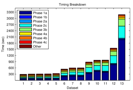
We ran our MapReduce code on the 13 networks described in §5.1. The runtimes are reported in Fig. 3, broken down by the phases of the algorithm. The largest real-world graph, uk-union (#12) with over 100 million vertices and over 4.6 billion edges, took less than 30 minutes to analyze. For all the networks, the most expensive step is Phase 1a, calculating the degree per node, because every edge in the edge list file generates two key-value pairs. For uk-union, this step takes over 12 minutes. Phases 1b and 2a are essentially constant time (approximately 30 seconds) because they process only the vertex degree file. Phase 2c (Create Sample Wedges) is the next most expensive step. Here we collect the edges adjacent to wedge centers, reading the entire edge list file again in the map phase; however, the wedge centers file created in Phase 2b minimizes the number of edges that are passed to reducers. Nevertheless, for the wedge centers with high degree, many edges are transmitted (though substantially less than the entire edge list). Phase 3b (Check Sample Wedge Closure) is the next most expensive, again reading the entire edge list file. The last few postprocessing steps are close to constant time (approximately 30-60 seconds each).

Fig. 3: Runtimes broken down by phases

Fig. 4: Correlation of the runtime to the number of edges. There is a setup cost of 225 seconds due to the MapReduce overhead and an incremental cost of 0.33 seconds per million edges.

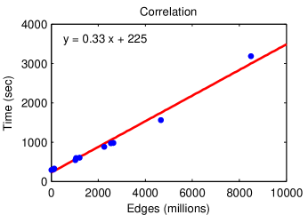
In an enumeration approach, we expect the runtimes to be proportional to the number of wedges. In that case, the sk-2005 (#10) would be the most expensive by an order of magnitude. For our method, however, the runtime is proportional to the number of edges. Fig. 4 shows that there is a near-linear relationship between the number of edges and the runtime. The x-axis is the number of edges (in millions) and the y-axis is the runtime. All 13 examples are included. We see that there is a constant cost of 225 seconds, which accounts for the MapReduce overhead and then an incremental cost of 0.33 seconds per million edges.

Comparisons to Other Methods

As one point of comparison, we ran Plantenga’s implementation that fully enumerates triangles [47] on several smaller graphs. The results are summarized in Tab. 3.

Table 3: Comparison of sampling and exact enumeration.

Id	Graph Name	Wedges	Run Time	Exact	Sampling	Sampling
		Checked	(sec.)	GCC	Error	Speed-up
1	amazon-2008	25%	158	0.2603	0.0001	1
2	ljournal-2008	19%	3,385	0.1228	0.0010	11
3	hollywood-2009	29%	21,665	0.3090	0.0006	72
4	hollywood-2011	27%	90,598	0.1761	0.0006	293

This implementation is efficient because it only checks wedges where the center degree is smallest, i.e., $(u,v,w)$ such that $d_{v}\leq d_{u}$ and $d_{v}\leq d_{w}$. This means that only one wedge per triangle is checked and moreover that many open wedges centered at high-degree nodes are ignored. The table lists the percentage of wedges that are checked for closure. The run times range from 3 minutes for the smallest graph, up to 25 hours for hollywood-2011 (2M nodes, 114M edges). Because this code enumerates every triangle, we can calculate the exact global clustering coefficient (GCC). The error from our sampling method is also reported. At a confidence level of 99.9%, using $k=2000$ samples yields an error of $\varepsilon=0.05$. The true errors are one to two orders of magnitude less than this worse case probabilistic bound. Finally, we observe the main advantage of sampling in terms of the observed speed-up, up to 293X for hollywood-2011. Larger graphs cannot be completed in a reasonable amount of time on our cluster.

Suri and Vassilvitskii [54] have an efficient enumeration method that was able to process two of the same data sets on a 1636-node Hadoop cluster: (a) ljournal-2008 required 5.33 minutes, and (b) twitter-2010 took 483 minutes. (In subsequent work, Arifuzzaman et al. [3, 2] have reduced the run time [43] were able to reduce the MapReduce run time to 213 minutes on 47 nodes.) On our 32-node cluster, our method requires approximately the same running time for the smaller data set (since most of the work is overhead) but required only 10 minutes for twitter-2010.

We also compare to in-memory methods. We used an SGI Altix UV 10 System with 4 Xeon 8-core nodes and 64 $\times$ 8GB memory, for a total of 32 cores and 512GB of memory. We consider two methods for exact node-level triangle counting on the twitter-2010 graph: (1) MTGL [6] using the algorithm described in [16] and (2) GraphLab/PowerGraph [37, 21]. On 32 cores, MTGL takes approximately 3.5 hours and consumes 125GB of memory. On 16 cores, GraphLab/PowerGraph takes approximately 17 minutes to run, and 430GB of memory at its peak usage, nearly maxing out the machine’s total memory. In both cases, just loading the graph takes 8–15 minutes. Compare these times to a total of 10 minutes using Hadoop and our inexact triangle-counting method.

The other class of methods for comparison are edge-sampling methods such as Doulion [59]. The basic idea is to sample a subset of edges and then run a triangle counting method (such as enumeration) on the reduced graph. Edge sampling has been compared to wedge sampling in serial [53]. Keeping 1 in 25 edges produces results that are roughly comparable to wedge sampling in time but with much greater variance in the GCC estimate. Keeping fewer edges yields savings in time but at the expense of much greater variance. Hence, we have not compared parallel implementations.

Fig. 5: Timings for variations. The variations are (1) Original algorithm, (2) Skip Phase 2b, (3) Skip Phase 3a.

Impact of Implementation Features

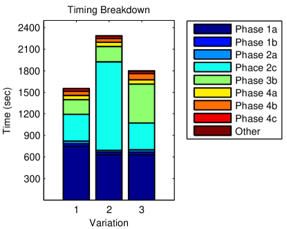
We have considered many alternatives during the implementation of the wedge sampling algorithm, and in this subsection we present the impact of two implementation features. The three versions of the code we compare are: (1) Original algorithm. (2) Skip Phase 2b. (3) Skip Phase 3a. We show results for uk-union in Fig. 5. Skipping Phase 2b means that every edge generates two messages in Phase 2c, increasing the time in that phase from 372 seconds to 1235 seconds (3X increase), twice as expensive as Phase 1a. Skipping Phase 3a means that every edge generates one message in Phase 3b, increasing the time in that phase from 207 seconds to 543 seconds (2.5X increase). Hence, taking measures to reduce the data that must be shuffled to the reducers has major pay-offs in terms of performance.

(a)

(b)

(c)

(d)

(e)

(f)

(g)

(h)

(i)

(j)

(k)

(l)

Fig. 6: Degree distributions by bin

5.4 Degree Distribution

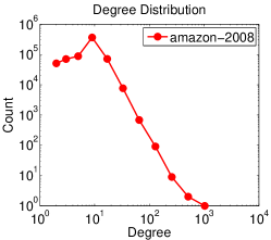
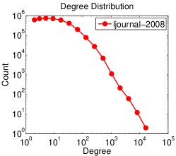
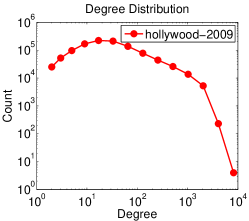
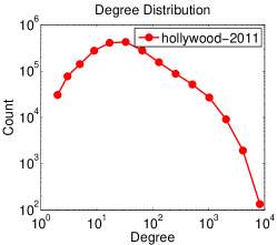
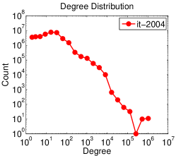
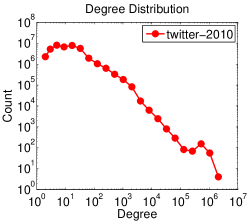
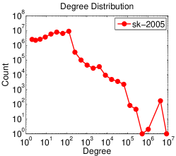
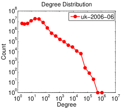
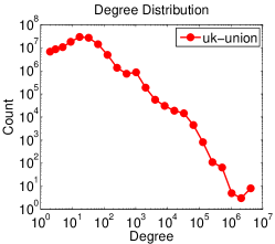
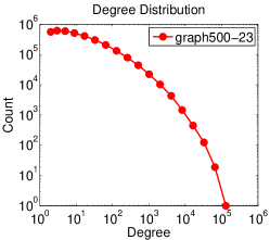
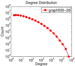
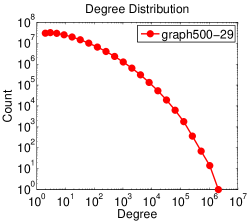
The output of Phase 1b yields the (binned) degree distribution. We show results for 12 networks in Fig. 6 (we omit uk-2006-05 because it is similar to uk-2006-06). For each data point, the x-coordinate is the minimum degree of the bin, and the y-coordinate is the total number of vertices in that bin.

The degree distributions can be roughly characterized as heavy-tailed. None of the real-world graphs are particularly smooth in the degree distribution, and some have odd spikes, especially in the tails (e.g., sk-2005, it-2004, uk-union). The artificial graphs (graph500-23/26/29) are extremely smooth; we know from analysis that the noisy version of Graph500 yields lognormal tails [52, 53].

5.5 Clustering Coefficients

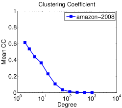
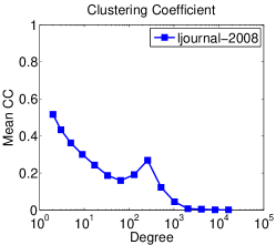
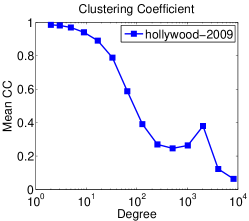
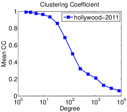
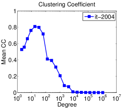
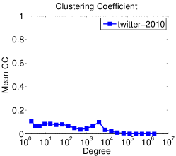
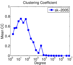
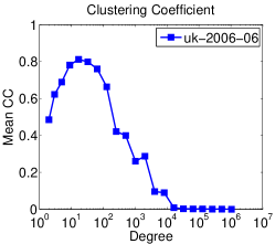
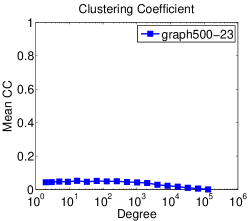
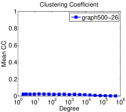
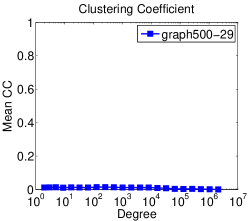
Clustering coefficients for each bin are displayed in Fig. 7. Here the x-coordinate is the minimum degree in the bin, and the y-coordinate is the average clustering coefficient for wedges with centers in that bin.

Social networks are well-known to have not only high clustering coefficients, but also clustering coefficients that tend to degrade as the degree increases. This can be seen in the following graphs: amazon-2008, ljournal-2008, hollywood-2009, hollywood-2011. The twitter-2010 graph is not as “social” in terms of clustering coefficient.

The web graphs (it-2004, uk-2006-06, uk-union, sk-2005) are interesting because the clustering coefficients seems to start low, increase, and then drop off quickly. This may be due to the design of web sites with many interconnected pages or to some artifact of the crawling process.

The Graph500 examples have overall low clustering coefficients and do not behave like the real-world graphs. The closest match is the twitter-2010 graph.

(a)

(b)

(c)

(d)

(e)

(f)

(g)

(h)

(i)

(j)

(k)

(l)

Fig. 7: Clustering coefficients by bin

5.6 Triangles

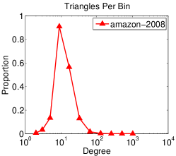
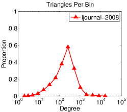
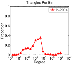
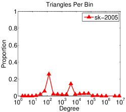
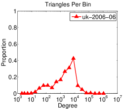
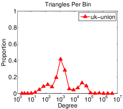
We also present the number of triangles per bin in Fig. 8. Here the x-coordinate is the minimum degree in the bin, and the y-coordinate is the proportion of triangles that have at least one vertex in that bin. Triangles may be counted more than once if they have different vertices in different bins.

It is interesting to observe where triangles come from. Even though low-degree nodes are the most plentiful, most of the triangles come from higher-degree. We can roughly sort the graphs into three categories.

There is only one graph where the triangles come from relatively low-degree vertices: amazon-2008. Here it seems that most triangles come from nodes with degrees between 4 and 80.

There are several graphs where the triangles come from the mid-range degrees: one social graph (ljournal-2008) and all the web graphs (it-2004, sk-2005, uk-2006-06, uk-union). The “double-spike” behavior of sk-2005 is interesting.

(a)

(b)

(c)

(d)

(e)

(f)

(g)

(h)

(i)

(j)

(k)

(l)

Fig. 8: Proportion of triangles in each bin

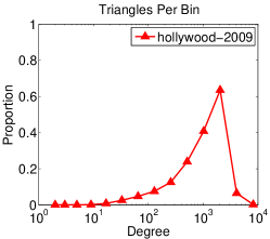
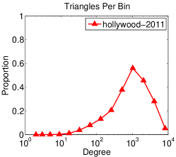
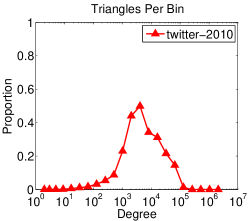
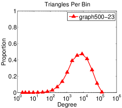
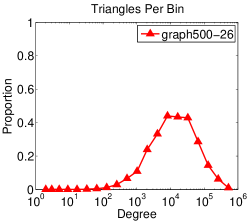
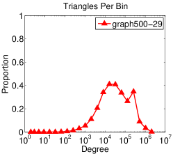
Finally, there are a few graphs where the vast majority of triangles involve the high-degree nodes. Both Hollywood graphs are of this type; note that 60% of the triangles involve one of the nodes in the bin starting at degree 1025. The Graph500 graphs also have most of the triangles coming from the highest degree nodes.

5.7 Triangle Statistics

An interesting feature of our wedge sampling techniques is that, in the case of a single bin, all the closed triangles are uniformly randomly sampled as well. Such a random sample can be used to analyze the characteristics of the triangles in the graph, going further than merely looking at their count. Examples of such studies can be found in [19], where full enumeration of the triangles was used. To avoid the burden of full enumeration a uniform sampling of the triangles can be used, as we showcase below.

For four example graphs, we ran our MapReduce code with a single bin ($\tau=1$ and $\omega=10^{7}$) and $k=5,000,000$ samples; we skipped phases 2b and 3a to avoid any data overflow problems in the configuration parameters. Runtimes and the number of triangles (expected to be roughly $k$ times the global clustering coefficient) are reporting in Tab. 4.

Table 4: Number of triangles from 5,000,000 wedge samples.

Graph Name	Time(s)	Triangles
uk-union	2618	33398
hollywood-2011	348	878719
graph500-26	845	46047
graph500-29	5487	25994

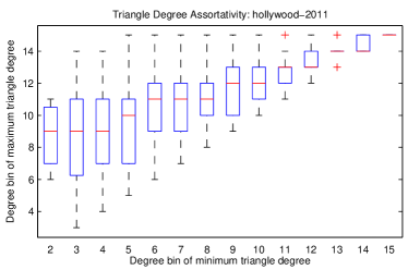
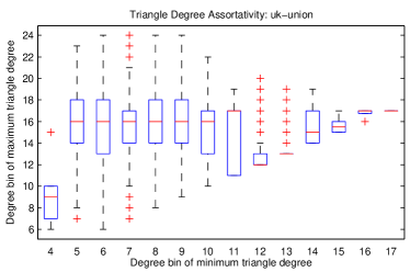
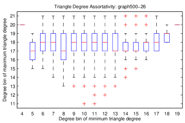
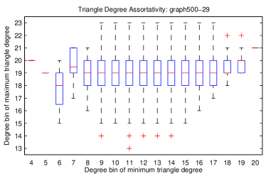
Using these sampled triangles, we can look at the degrees of the vertices. Each triangle has a minimum, middle, and maximum degree. We analyze the degree assortativity of the vertices of the triangles by comparing the minimum and maximum degrees in Fig. 9. Specifically, we assign each vertex to a degree bin, using (4) with $\tau=2$ and $\omega=2$. We group all triangles with the same minimum degree bin together. The box plot shows the statistics of the bin for the maximum degree: the central mark (red) is the median max-degree, while the edges of the (blue) box are the 25th and 75th percentiles. The whiskers extend to the most extreme points considered not to be outliers, and the outliers (red plus marks) are plotted individually.

Observe that the social network, hollywood-2011, shows an assortative relation between the maximum and minimum for the hollywood graph, since the two quantities rise gradually together. For the uk-union web graph on the other hand, the average maximum degree is essentially invariant to the minimum degree. These findings are consistent with the results in [19] about networks with high global clustering coefficients having degree assortative triangles, while this assortativity cannot be observed in networks with low clustering coefficients. Here, we were able to observe the same trend on these massive graphs using sampling in a much more efficient way, avoiding the enumeration burden. We see that the Graph500 networks also have almost no assortativity between the minimum and maximum degrees and therefore do not have the characteristics of a social network.

(a)

(b)

(c)

(d)

Fig. 9: Triangle Degree Assortativity

6 Conclusions

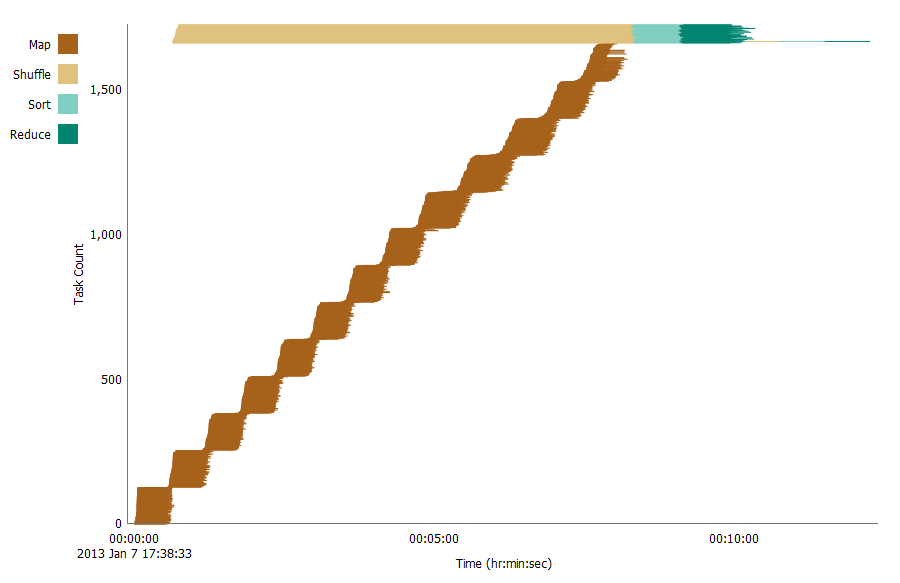
We have shown that wedge-based sampling can be scaled to massive graphs in the MapReduce framework. On a relatively small MapReduce cluster (32 nodes), we have analyzed graphs with up to 240M edges, 8.5B edges, 5.2T wedges, and 447B triangles. Even the largest graph was analyzed in less than one hour, and most took only a few minutes. Fig. 10 shows a timing analysis of the MapReduce tasks [65] for Phase 1a on the uk-union graph. Mapper tasks run in waves of 128 parallel jobs, equal to the number of mapper slots available on the cluster. Note that a larger cluster would be able to run more Map tasks in parallel, decreasing the overall runtime. To the best of our knowledge, these are the largest triangle-based calculations performed to date.

Fig. 10: Task breakdown for Phase 1a on uk-union on 32 Hadoop nodes.

Unlike enumeration techniques that need to at least validate every triangle and more often have cost proportional to the number of wedges, our method is linear in the number of edges. The most expensive component of the wedge-based sampling is finding the degree of each vertex (Phase 1a); reducing the time for this is a topic for future study. On our cluster, the time is approximately 0.33 seconds per million edges, plus a fixed cost of 225 seconds for overhead. Because we are using MapReduce, we never need to fit the entire graph into memory — we only need to be able to stream through all the edges.

Our MapReduce implementation requires a total of eight MapReduce jobs, three of which do most of the work because they read the entire edge list (Phases 1a, 2c, and 3b) and two of which are optional (Phases 4a and 4b, which are labeling the degrees of the sampled triangles). We have striven to minimize the data being shuffled in each phase by using special data structures to filter the edges.

Using our code, we are able to compute the degree distribution, approximate the binned degree-wise clustering coefficient and the number of triangles per bin. Additionally, we can analyze the characteristics of the triangles (e.g. degree assortativity). As part of our analysis, we have analyzed the graphs used in the Graph500 benchmark. We are able to give a more detailed understanding of the empirical properties of the generator and compare it to real-world data; this is potentially helpful in determining if performance on the benchmark data is indicative of performance on real-world data.

References

- [1] Apache Software Foundation, Hadoop. http://hadoop.apache.org/, 2012.
- [2] S. Arifuzzaman, M. Khan, and M. Marathe, Poster: Parallel algorithms for counting triangles and computing clustering coefficients, in High Performance Computing, Networking, Storage and Analysis (SCC), 2012, pp. 1450–1450.
- [3] S. M. Arifuzzaman, M. Khan, and M. V. Marathe, PATRIC: A parallel algorithm for counting triangles and computing clustering coefficients in massive networks, NDSSL Technical Report 12-042, Network Dynamics and Simulation Science Laboratory, Virginia Polytechnic Institute and State University, July 2012.
- [4] H. Avron, Counting triangles in large graphs using randomized matrix trace estimation, in KDD-LDMTA’10, 2010.
- [5] Z. Bar-Yossef, R. Kumar, and D. Sivakumar, Reductions in streaming algorithms, with an application to counting triangles in graphs, in SODA’02, 2002, pp. 623–632.
- [6] B. W. Barrett, J. W. Berry, R. C. Murphy, and K. B. Wheeler, Implementing a portable multi-threaded graph library: The MTGL on Qthreads, in IPDPS 2009: IEEE International Symposium on Parallel & Distributed Processing, 2009, pp. 1–8.
- [7] L. Becchetti, P. Boldi, C. Castillo, and A. Gionis, Efficient semi-streaming algorithms for local triangle counting in massive graphs, in KDD’08, 2008, pp. 16–24.
- [8] P. Boldi, B. Codenotti, M. Santini, and S. Vigna, UbiCrawler: A scalable fully distributed web crawler, Software: Practice & Experience, 34 (2004), pp. 711–726.
- [9] P. Boldi, M. Rosa, M. Santini, and S. Vigna, Layered label propagation: A multiresolution coordinate-free ordering for compressing social networks, in WWW’11: Proceedings of the 20th international conference on World Wide Web, ACM Press, 2011.
- [10] P. Boldi, M. Santini, and S. Vigna, A large time-aware graph, SIGIR Forum, 42 (2008), pp. 33–38.
- [11] P. Boldi and S. Vigna, The webgraph framework I: Compression techniques, in WWW’04: Proceedings of the 13th International Conference on World Wide Web, ACM Press, 2004, pp. 595–602.
- [12] L. S. Buriol, G. Frahling, S. Leonardi, A. Marchetti-Spaccamela, and C. Sohler, Counting triangles in data streams, in PODS’06: Proceedings of the twenty-fifth ACM SIGMOD-SIGACT-SIGART Symposium on Principles of Database Systems, 2006, pp. 253–262.
- [13] N. Chiba and T. Nishizeki, Arboricity and subgraph listing algorithms, SIAM J. Comput., 14 (1985), pp. 210–223.
- [14] F. Chierichetti, R. Kumar, S. Lattanzi, M. Mitzenmacher, A. Panconesi, and P. Raghavan, On compressing social networks, in KDD ’09: Proceedings of the 15th ACM SIGKDD international conference on Knowledge discovery and data mining, ACM, 2009, pp. 219–228.
- [15] S. Chu and J. Cheng, Triangle listing in massive networks and its applications, in KDD’11: Proceedings of the 17th ACM SIGKDD International Conference on Knowledge Discovery and Data Mining, New York, 2011, ACM, pp. 672–680.
- [16] J. Cohen, Graph twiddling in a MapReduce world, Computing in Science and Engineering, 11 (2009), pp. 29–41.
- [17] J. Dean and S. Ghemawat, MapReduce: Simplified data processing on large clusters, Communications of the ACM, 51 (2008), pp. 107–113.
- [18] D. Dubhashi and A. Panconesi, Concentration of Measure for the Analysis of Randomized Algorithms, Cambridge University Press, 2009.
- [19] N. Durak, A. Pinar, T. G. Kolda, and C. Seshadhri, Degree relations of triangles in real-world networks and graph models, in CIKM ’12: Proceedings of the 21st ACM International Conference on Information and Knowledge Management, CIKM ’12, New York, NY, USA, 2012, ACM, pp. 1712–1716.
- [20] D. V. Foster, J. G. Foster, P. Grassberger, and M. Paczuski, Clustering drives assortativity and community structure in ensembles of networks, Phys. Rev. E, 84 (2011), p. 066117.
- [21] J. Gonzalez, Y. Low, H. Gu, D. Bickson, and C. Guestrin, Powergraph: Distributed graph-parallel computation on natural graphs, in Proc. of the 10th USENIX conference on Operating systems design and implementation, 2012, pp. 17–30.
- [22] W. Guo and S. Kraines, A random network generator with finely tunable clustering coefficient for small-world social networks, in CASON ’09: International Conference on Computational Aspects of Social Networks, June 2009, pp. 10–17.
- [23] W. Hoeffding, Probability inequalities for sums of bounded random variables, Journal of the American Statistical Association, 58 (1963), pp. 13–30.
- [24] Z. Huang, Link prediction based on graph topology: The predictive value of generalized clustering coefficient. Social Science Research Network, 2010.
- [25] M. Jha, C. Seshadhri, and A. Pinar, A space efficient streaming algorithm for triangle counting using the birthday paradox, in Proceedings of the 19th ACM SIGKDD International Conference on Knowledge Discovery and Data Mining, KDD ’13, New York, NY, USA, 2013, ACM, pp. 589–597.
- [26] , When a graph is not so simple: Counting triangles in multigraph streams, 2013. arXiv:1310.7665.
- [27] H. Jowhari and M. Ghodsi, New streaming algorithms for counting triangles in graphs, in COCOON’05: Computing and Combinatorics, L. Wang, ed., vol. 3595 of Lecture Notes in Computer Science, Springer Berlin Heidelberg, 2005, pp. 710–716.
- [28] U. Kang, C. Tsourakakis, and C. Faloutsos, Pegasus: A peta-scale graph mining system implementation and observations, in ICDM ’09. Ninth IEEE International Conference on Data Mining, Dec. 2009, pp. 229–238.
- [29] M. N. Kolountzakis, G. L. Miller, R. Peng, and C. E. Tsourakakis, Efficient triangle counting in large graphs via degree-based vertex partitioning, Internet Mathematics, 8 (2012), pp. 161–185.
- [30] H. Kwak, C. Lee, H. Park, and S. Moon, What is Twitter, a social network or a news media?, in WWW ’10: Proceedings of the 19th international conference on World wide web, New York, NY, USA, 2010, ACM, pp. 591–600.
- [31] M. Latapy, Main-memory triangle computations for very large (sparse (power-law)) graphs, Theoretical Computer Science, 407 (2008), pp. 458–473.
- [32] S. Lattanzi, B. Moseley, S. Suri, and S. Vassilvitskii, Filtering: a method for solving graph problems in MapReduce, in Proceedings of the 23rd ACM symposium on Parallelism in algorithms and architectures, SPAA ’11, New York, NY, USA, 2011, ACM, pp. 85–94.
- [33] J. Leskovec, D. Chakrabarti, J. Kleinberg, C. Faloutsos, and Z. Ghahramani, Kronecker graphs: An approach to modeling networks, Journal of Machine Learning Research, 11 (2010), pp. 985–1042.
- [34] J. Lin, Mapreduce is good enough? If all you have is a hammer, throw away everything that’s not a nail! arXiv:1209.2191, Sept. 2012.
- [35] J. Lin and C. Dyer, Data-Intensive Text Processing with MapReduce, Morgan & Claypool Publishers, 2010. Citing post-production version of manuscript dated Sept. 6, 2012, available at http://lintool.github.com/MapReduceAlgorithms/ed1n.html.
- [36] J. Lin and M. Schatz, Design patterns for efficient graph algorithms in MapReduce, in MLG’10: Proceedings of the Eighth Workshop on Mining and Learning with Graphs, MLG ’10, New York, NY, USA, 2010, ACM, pp. 78–85.
- [37] Y. Low, J. Gonzalez, A. Kyrola, D. Bickson, C. Guestrin, and J. M. Hellerstein, GraphLab: A new framework for parallel machine learning. arXiv:1006.4990, 2010.
- [38] M. E. J. Newman, The structure of scientific collaboration networks, Proceedings of the National Academy of Sciences, 98 (2001), pp. 404–409.
- [39] M. E. J. Newman and J. Park, Why social networks are different from other types of networks, Phys. Rev. E, 68 (2003), p. 036122.
- [40] M. E. J. Newman, S. H. Strogatz, and D. J. Watts, Random graphs with arbitrary degree distributions and their applications, Phys. Rev. E, 64 (2001), p. 026118.
- [41] R. N. Onody and P. A. de Castro, Complex network study of Brazilian soccer players, Phys. Rev. E, 70 (2004), p. 037103.
- [42] R. Pagh and C. Tsourakakis, Colorful triangle counting and a MapReduce implementation, Information Processing Letters, 112 (2012), pp. 277–281.
- [43] H.-M. Park and C.-W. Chung, An efficient MapReduce algorithm for counting triangles in a very large graph, in CIKM’13: Proceedings of the 22nd ACM international conference on Conference on information & knowledge management, Association for Computing Machinery, 2013, pp. 539–548.
- [44] M. Patrascu, Towards polynomial lower bounds for dynamic problems, in Proceedings of the 42nd ACM symposium on Theory of computing, 2010, pp. 603–610.
- [45] R. Pearce, M. Gokhale, and N. M. Amato, Scaling techniques for massive scale-free graphs in distributed (external) memory, in Proc. Int. Par. and Dist. Proc. Symp. (IPDPS), May 2013.
- [46] T. Plantenga, MapReduce R-MAT graph generator. private communication, 2012.
- [47] , Inexact subgraph isomorphism in MapReduce, Journal of Parallel and Distributed Computing, 73 (2013), pp. 164 – 175.
- [48] A. Sala, L. Cao, C. Wilson, R. Zablit, H. Zheng, and B. Y. Zhao, Measurement-calibrated graph models for social network experiments, in WWW ’10: Proceedings of the 19th international conference on World wide web, 2010, pp. 861–870.
- [49] T. Schank and D. Wagner, Approximating clustering coefficient and transitivity, Journal of Graph Algorithms and Applications, 9 (2005), pp. 265–275.
- [50] , Finding, counting and listing all triangles in large graphs, an experimental study, in Experimental and Efficient Algorithms, Springer Berlin / Heidelberg, 2005, pp. 606–609.
- [51] C. Seshadhri, T. G. Kolda, and A. Pinar, Community structure and scale-free collections of Erdös-Rényi graphs, Physical Review E, 85 (2012), p. 056109.
- [52] C. Seshadhri, A. Pinar, and T. G. Kolda, An in-depth study of stochastic Kronecker graphs, in ICDM 2011: Proceedings of the 2011 IEEE International Conference on Data Mining, 2011, pp. 587–596.
- [53] C. Seshadhri, A. Pinar, and T. G. Kolda, Triadic measures on graphs: The power of wedge sampling, in SIAM Conference on Data Mining (SDM), 2013. Preprint available at http://arxiv.org/abs/1202.5230.
- [54] S. Suri and S. Vassilvitskii, Counting triangles and the curse of the last reducer, in WWW ’11: Proceedings of the 20th International Conference on World Wide Web, New York, NY, USA, 2011, ACM, pp. 607–614.
- [55] K. Tangwongsan, A. Pavan, and S. Tirthapura, Parallel triangle counting in massive streaming graphs, in CIKM13: Proceedings of the 22nd ACM international conference on Conference on information & knowledge management, Association for Computing Machinery, 2013, pp. 781–786.
- [56] C. Tsourakakis, P. Drineas, E. Michelakis, I. Koutis, and C. Faloutsos, Spectral counting of triangles in power-law networks via element-wise sparsification, in ASONAM ’09. International Conference on Advances in Social Network Analysis and Mining, 2009., July 2009, pp. 66–71.
- [57] C. Tsourakakis, M. N. Kolountzakis, and G. Miller, Triangle sparsifiers, Journal of Graph Algorithms and Applications, 15 (2011), pp. 703–726.
- [58] C. E. Tsourakakis, Fast counting of triangles in large real networks, without counting: Algorithms and laws, in ICDM 2008: Proceedings of the 8th IEEE International Conference on Data Mining, 2008, pp. 608–617.
- [59] C. E. Tsourakakis, U. Kang, G. L. Miller, and C. Faloutsos, Doulion: counting triangles in massive graphs with a coin, in KDD ’09, 2009, pp. 837–846.
- [60] J. Ugander, B. Karrer, L. Backstrom, and C. Marlow, The anatomy of the Facebook social graph. arXiv:1111.4503v1, Nov. 2011.
- [61] D. Watts and S. Strogatz, Collective dynamics of ‘small-world’ networks, Nature, 393 (1998), pp. 440–442.
- [62] V. V. Williams and R. Williams, Subcubic equivalences between path, matrix and triangle problems, in Proceedings of the IEEE Annual Symposium on Foundations of Computer Science, 2010, pp. 645–654.
- [63] B. Wu, Y. Dong, Q. Ke, and Y. Cai, A parallel computing model for large-graph mining with MapReduce, in ICNC’11: 2011 Seventh International Conference on Natural Computation, vol. 1, July 2011, pp. 43–47.
- [64] J.-H. Yoon and S.-R. Kim, Improved sampling for triangle counting with mapreduce, in Convergence and Hybrid Information Technology, G. Lee, D. Howard, and D. Slezak, eds., vol. 6935 of Lecture Notes in Computer Science, Springer Berlin / Heidelberg, 2011, pp. 685–689.
- [65] A. Yoshimura, Hadoop JobInfo tool. private communication, 2012.
- [66] Z. Zhao, G. Wang, A. Butt, M. Khan, V. Kumar, and M. Marathe, SAHAD: Subgraph analysis in massive networks using Hadoop, in IPDPS’12: 2012 IEEE 26th International Parallel Distributed Processing Symposium, May 2012, pp. 390–401.
- [67] Graph 500. www.graph500.org.