Non-Homogeneous Local $T1$ Theorem: Dual Exponents

Abstract.

We provide an alternative proof of a (local) $T1$ theorem for dual exponents in the non-homogeneous setting of upper doubling measures. This previously known theorem provides necessary and sufficient conditions for the $L^{p}$-boundedness of Calderón–Zygmund operators in the described setting, and the novelty lies in the method of proof.

1. Introduction

1.1. Background and motivation

The subject of local $Tb$ theorems in the classical setting of $\mathbf{R}^{n}$ with Lebesgue measure is rather well understood by now. We refer, in particular, to [hytonen_nazarov] and to [MR1934198, 1011.1747, MR2474120, 0705.0840, lv-perfect, 1209.4161]. These theorems extend the David–Journé $T1$ Theorem [MR763911], and the $Tb$ theorem of Christ [MR1096400] by giving flexible conditions under which an operator $T$ with a Calderón–Zygmund kernel extends to a bounded linear operator on $L^{2}$. By ‘local’ we understand that the $Tb$ conditions involve a family of test functions $b_{Q}$, one for each cube $Q$, which should satisfy a non-degeneracy condition on its ‘own’ $Q$. Furthermore, both $b_{Q}$ and $Tb_{Q}$ are subject to normalized integrability conditions on $Q$ (with suitable exponents). Symmetric assumptions are imposed on $T^{*}$.

In the non-homogeneous setting less is know. In the relevant literature [1011.0642, 1201.0648, MR1909219] one usually encounters stronger $L^{\infty}(\mathbf{R}^{n})$ (sometimes $\mathrm{BMO}$) conditions on $Tb_{Q}$’s, as well as on test functions $b_{Q}$. In the search after relaxation of these conditions one faces complications that arise from the feature that the underlying measure $\mu$ need not be doubling.

We provide an alternative proof of a local $T1$ theorem—which is, in fact, a $T1$ theorem in its local formulation—in the non-homogeneous setting of upper doubling measures, [0909.3231, 0911.4387]. The local testing functions are indicators of cubes: $b_{Q}=\mathbf{1}_{Q}$, and integrability conditions on $\mathbf{1}_{Q}T\mathbf{1}_{Q}$ and $\mathbf{1}_{Q}T^{*}\mathbf{1}_{Q}$ are those of dual exponents $1<p_{1}<\infty$ and $p_{2}=p_{1}/(p_{1}-1)$. This result is already known and available in the literature, see Remark 1.6, and the motivation stems from the fact that our novel proof possibly lends itself to other situations. In particular, a non-homogeneous local $Tb$ theorem, say, for dual exponents, has not yet been established, and it seems plausible that the new techniques in the present paper can be used to attack this open and difficult problem.

More precisely, our proof relies upon a so called corona decomposition, adapted to the maximal averages of given two functions $f_{1}$ and $f_{2}$. The advantage of this approach is that one has powerful quasi orthogonality inequalities, useful throughout the proof. A direct argument can be used to control a difficult ‘inside’ term, thereby we avoid the typical use of paraproducts and Carleson measures. This argument can be viewed as an extension of its ‘homogeneous’ counterparts that are developed in [lv-perfect, 1209.4161].

1.2. A local $T1$ theorem

Let $\mu$ be a compactly supported Borel measure on $\mathbf{R}^{n}$. We assume the upper doubling conditions of Hytönen [0909.3231]: there is a dominating function $\lambda\;:\;\mathbf{R}^{n}\times\mathbf{R}_{+}\to\mathbf{R}_{+}$, and a constant $C_{\lambda}>0$, such that for all $x\in\mathbf{R}^{n}$ and $r>0$:

(1.1) $$\mu(B(x,r))\leq\lambda(x,r)\leq C_{\lambda}\lambda(x,r/2)\,.$$

Moreover, we assume that $r\mapsto\lambda(x,r)$ is non-decreasing for all $x\in\mathbf{R}^{n}$. The number $d=\log_{2}C_{\lambda}$ can be thought of as the dimension of $\mu$.

We assume that a linear operator $T$ is bounded on $L^{2}(d\mu)$, and it is adapted to $\lambda$ in the following sense. There is a kernel $K\;:\;\mathbf{R}^{n}\times\mathbf{R}^{n}\to\mathbf{R}$ such that for all compactly supported $f\in L^{2}(\mathbf{R}^{n})$,

$$Tf(x)=\int_{\mathbf{R}^{n}}K(x,y)f(y)\,d\mu(y)\,,\qquad x\not\in\mathrm{supp}(f).$$

We assume that these kernel estimates hold for some $\eta\in(0,1)$:

(1.2) $$\lvert K(x,y)\rvert\leq\min\bigg{\{}\frac{1}{\lambda(x,\lvert x-y\rvert)},\frac{1}{\lambda(y,\lvert x-y\rvert)}\bigg{\}}\,,\qquad x\neq y\,,$$

(1.3) $$\lvert K(x,y)-K(x^{\prime},y)\rvert\leq\frac{\lvert x-x^{\prime}\rvert^{\eta}}{\lvert x-y\rvert^{\eta}\lambda(x,\lvert x-y\rvert)},\qquad\lvert x-y\rvert\geq 2\lvert x-x^{\prime}\rvert\,,$$

and

$$\lvert K(x,y)-K(x,y^{\prime})\rvert\leq\frac{\lvert y-y^{\prime}\rvert^{\eta}}{\lvert x-y\rvert^{\eta}\lambda(y,\lvert x-y\rvert)},\qquad\lvert x-y\rvert\geq 2\lvert y-y^{\prime}\rvert\,.$$

The operator $T$ is said to be a Calderón–Zygmund operator. We are interested in quantitative estimates for the operator norm of $T$ on $L^{p}(\mu)$ for $1<p<\infty$, and the following hypothesis, together with kernel assumptions, provides the essential quantitative information.

• Local Testing Condition Hypothesis. For given two exponents $p_{1},p_{2}\in(1,\infty)$, there is a constant $\mathbf{T}_{\textup{loc}}$ as follows. For all cubes $Q$ in $\mathbf{R}^{n}$,

  (1.4) $$\int_{Q}\lvert T\mathbf{1}_{Q}\rvert^{p_{1}}\,d\mu(x)\leq\mathbf{T}_{\mathbf{loc}}^{p_{1}}\mu(Q)\,,\qquad\int_{Q}\lvert T^{\ast}\mathbf{1}_{Q}\rvert^{p_{2}}\,d\mu(x)\leq\mathbf{T}_{\textup{loc}}^{p_{2}}\mu(Q)\,.$$

We provide a novel proof of the following previously known theorem.

1.5 Theorem.

Let $T$ be a Calderón–Zygmund operator. Fix $1<p_{1},p_{2}<\infty$, $1/p_{1}+1/p_{2}\leq 1$. Assume the following two conditions (1)–(2):

• $T$ is (a priori) bounded on $L^{p_{1}}(d\mu)$;

• $T$ satisfies a Local Testing Condition Hypothesis with exponents $p_{1}$ and $p_{2}$.

Under these assumptions, we have a quantitative norm estimate

$$\mathbf{T}:=\lVert T\rVert_{L^{p_{1}}(d\mu)\to L^{p_{1}}(d\mu)}\lesssim 1+\mathbf{T}_{\textup{loc}}\,,$$

where the implied constant depends on $n,p_{1},p_{2},\eta,\mu$.

In the sequel, unless otherwise specified, we assume that $p_{1}$ and $p_{2}$ are in duality: $p_{2}=\frac{p_{1}}{p_{1}-1}$.

1.6 Remark.

Theorem 1.5 is known and available in the literature. Indeed, under the assumptions of this theorem, it is straightforward to verify that $T$ satisfies a ‘weak boundedness property’ and ‘testing conditions’, namely for all cubes $Q$ in $\mathbf{R}^{n}$, and an appropriate $\sigma\geq 1$,

(1.7) $$\bigg{\lvert}\int_{Q}T\mathbf{1}_{Q}\,d\mu\bigg{\rvert}\leq\mathbf{T}_{\textup{loc}}\mu(Q)\,,\qquad T\mathbf{1}\in\mathrm{BMO}_{\sigma}^{p_{1}}(\mu),\qquad T^{*}\mathbf{1}\in\mathrm{BMO}_{\sigma}^{p_{2}}(\mu)\,;$$

we refer to Remark 2.10 for further details. It remains to apply a non-homogeneous $T1$ theorem, see [NTV1] or [0809.3097, $Tb$ theorem 2] for $\lambda(x,r)=r^{d}$ dominating the measure, and [MR2990130, Theorem 2.1] for the general case. Moreover, by using the last theorem, it is even possible to relax the integrability conditions in (1.4) to exponents $p_{1}=1=p_{2}$. Let us also remark that the case of $p_{1}=2=p_{2}$ has been addressed in [MR2956255] with a function $\lambda(x,r)=\max\{\delta(x)^{d},r^{d}\}$ dominating the measure, where $\delta(x)=\mathrm{dist}(x,\mathbf{R}^{n}\setminus H)$ for an an open set $H$ in $\mathbf{R}^{n}$.

1.8 Remark.

The $p$-independence property of Calderón–Zygmund operators, i.e., if their $L^{2}$ boundedness is equivalent to their $L^{p}$ boundedness, has been addressed, for instance, in [MR2957235, HuMengYang]. It is an interesting question, if our proof can be adapted to obtain a quantitative $p$-independence result for Calderón–Zygmund operators, under an appropriate set of local testing hypotheses.

1.3. Structure of the paper

We use the non-homogeneous techniques of [NTV1], in particular, good and bad cubes are applied in a partially novel manner. Martingale techniques, including $L^{p}$ estimates for martingale transforms and Stein’s ineguality, are fundamental. These techniques are also applied in a related paper [1201.0648], from which we borrow also some other ideas, e.g., treatments of ‘separated’ and ‘nearby’ terms. Our main technical contribution is treatment of the most difficult ‘inside’ term by a strong definition of goodness and a corona decomposition, avoiding (a) explicit construction of paraproduct operators; and (b) Carleson embedding theorems.

The heart of the matter is estimation of a form $\lvert\langle Tf_{1},f_{2}\rangle\rvert$, where $f_{j}$’s are perturbed functions, supported on large dyadic cubes $Q_{j,0}\in\mathcal{D}_{j}$. Here $\mathcal{D}_{j}$ is a random dyadic system. The perturbation is simply a projection to good cubes, and results in that the usual martingale differences $\Delta_{Q}f_{j}$ vanish if $Q\subset Q_{j,0}$ is a bad. After a probabilistic absorption argument, the focus will be on a triangular form

$$\Big{\lvert}\sum_{\begin{subarray}{c}P,Q\textup{ good}\end{subarray}}\mathbf{1}_{\ell Q\leq\ell P}\cdot\langle T\Delta_{P}f_{1},\Delta_{Q}f_{2}\rangle\Big{\rvert}\,,$$

where always $P\subset Q_{1,0}$ and $Q\subset Q_{2,0}$. This form is further split into ‘inside’, ‘separated’, and ‘nearby’ terms. The analysis of the inside term, in which $Q$ is deeply inside $P$, is taken up in sections 5 and 6—the argument is transparent, and our strong definition of goodness of cubes has a key role. The construction of paraproducts is avoided, and even Carleson embedding theorems are not needed; in this we follow [1108.2319, 1201.4319]. We apply a corona decomposition, and the associated stopping tree is constructed in Section 4, where we also record the basic ‘quasi-orthogonality’ properties. The separated term, in which $Q$ is always far away from $P$, is analysed in Section 7, and the (usual) goodness is crucial. Throughout sections 8–10, we treat the nearby term, where cubes are close to each other both in position and size. The usual surgery is performed.

Acknowledgment.

The authors would like to thank Tuomas Hytönen and Henri Martikainen for indicating the connection of Theorem 1.5 to the $T1$ theorems that are available in the literature.

2. Preliminaries

2.1. Notation

The implied constants are allowed to depend upon parameters $r,n,p_{1},p_{2},\eta,\mu$. The distances are measured in supremum norm, $\lvert x\rvert=\rVert x\rVert_{\infty}$ for $x\in\mathbf{R}^{n}$. We denote $L^{p}=L^{p}(d\mu)$ if $1\leq p\leq\infty$. For a cube $Q$ and $f\in L^{1}_{\textup{loc}}$, write $\langle f\rangle_{Q}:=\mu(Q)^{-1}\int_{Q}f\;d\mu$ with the convention $\langle f\rangle_{Q}=0$ if $\mu(Q)=0$. The side length of a cube $Q$ is written as $\ell Q$, and the midpoint as $x_{Q}$. The ‘long distance’ between cubes $Q$ and $P$ is $D(Q,P)=\ell Q+\mathrm{dist}(Q,P)+\ell P$.

A ‘dyadic cube’ is any cube in either random grid $\mathcal{D}_{j}$ with $j\in\{1,2\}$, Section 2.2. By $\mathcal{D}_{j,k}$ we denote those dyadic cubes $Q\in\mathcal{D}_{j}$ for which $\ell Q=2^{k}$, $k\in\mathbf{Z}$. The dyadic children of $Q\in\mathcal{D}_{j}$ are $\{Q_{1},\ldots,Q_{2^{n}}\}=\textup{ch}(Q)$, its dyadic parent is $\pi_{j}Q=\pi_{j}^{1}Q$, and $\pi_{j}^{t}Q=\pi_{j}(\pi_{j}^{t-1}Q)$ for $t\in\{2,3,\ldots\}$. For $\mathcal{S}_{j}\subset\mathcal{D}_{j}$ the family $\textup{ch}_{\mathcal{S}_{j}}(S)=\textup{ch}^{1}_{\mathcal{S}_{j}}(S)$ consists of the $\mathcal{S}_{j}$-children of $S\in\mathcal{S}_{j}$: the maximal cubes in $\mathcal{S}_{j}$ that are strictly contained in $S$. We also denote $\textup{ch}_{\mathcal{S}_{j}}^{0}(S)=\{S\}$ and, for $t>1$, write $S^{\prime}\in\textup{ch}^{t}_{\mathcal{S}_{j}}(S)$ if $S^{\prime}\in\textup{ch}_{\mathcal{S}_{j}}(S^{\prime\prime})$ for some $S^{\prime\prime}\in\textup{ch}^{t-1}_{\mathcal{S}_{j}}(S)$. For any cube $Q$ which is contained in a cube in $\mathcal{S}_{j}$, we take $\pi_{\mathcal{S}_{j}}Q=\pi_{\mathcal{S}_{j}}^{0}Q$ to be the $\mathcal{S}_{j}$-parent of $Q$: the minimal $\mathcal{S}_{j}$-cube containing $Q$ (if $Q$ is not contained in a cube in $\mathcal{S}_{j}$, we set $\pi_{\mathcal{S}_{j}}Q=\mathbf{R}^{n}$). For $t\geq 1$ and any cube $Q$, contained in at least $t+1$ cubes in $\mathcal{S}_{j}$, we let $\pi_{\mathcal{S}_{j}}^{t}Q$ to be $\pi_{\mathcal{S}_{j}}^{t-1}S^{\prime}$, where $\pi_{\mathcal{S}_{j}}Q\in\textup{ch}_{\mathcal{S}_{j}}(S^{\prime})$.

2.2. Random grids

We use the foundational tool of random grids, initiated by Nazarov–Treil–Volberg [MR1909219], which has in turn been used repeatedly. We refer, e.g., to [MR1756958, 1201.4319, 0911.4387, MR2912709]. Throughout the paper, we shall use two random dyadic grids (systems) $\mathcal{D}_{j}$, $j\in\{1,2\}$. A third random grid $\mathcal{D}_{3}$ appears at the very end. These are constructed as follows; we refer to [1108.5119] for further details.

The random grids $\mathcal{D}_{j}$ are parametrized by sequences $\omega_{j}\in(\{0,1\}^{n})^{\mathbf{Z}}$, $j\in\{1,2,3\}$, where we tacitly assume three independent copies of $(\{0,1\}^{n})^{\mathbf{Z}}$. More precisely, for a cube $\widehat{Q}\in\widehat{\mathcal{D}}$ in the standard dyadic grid, the position of an $\omega_{j}$-translated cube is

$$Q=\widehat{Q}\dot{+}\omega_{j}:=\widehat{Q}+\sum_{k\,:\,2^{-k}<\ell\widehat{Q}}2^{-k}\omega_{j,k}\,,$$

which is a function of $\omega_{j}\in(\{0,1\}^{n})^{\mathbf{Z}}$. A dyadic grid (system)

$$\mathcal{D}_{j}=\mathcal{D}(\omega_{j})=\{\widehat{Q}\dot{+}\omega_{j}\,:\,\widehat{Q}\in\widehat{\mathcal{D}}\}$$

is the family of these $\omega_{j}$-translated cubes. The natural uniform probability measure $\mathbf{P}_{\omega_{j}}$ is placed upon the respective copy of $(\{0,1\}^{n})^{\mathbf{Z}}$. Each component $\omega_{j,k}$, $k\in\mathbf{Z}$, has an equal probability $2^{-n}$ of taking any of the $2^{n}$ values, and all components are independent of each other. The expectation with respect to $\mathbf{P}_{\omega_{j}}$ is denoted by $\mathbf{E}_{\omega_{j}}$. We will usually simply write $P$ or $S$ for a cube in $\mathcal{D}_{1}$, and $Q$ or $R$ for a cube in $\mathcal{D}_{2}$, instead of the heavier notation $\widehat{Q}\dot{+}\omega_{j}$ with $\widehat{Q}\in\widehat{\mathcal{D}}$.

Choose, once and for all, a constant $\gamma\in(0,1)$ such that

(2.1) $$d\gamma/(1-\gamma)\leq\eta/4,\quad\gamma\leq\frac{\eta}{2(d+\eta)}\,,\qquad d=\log_{2}C_{\lambda}\,.$$

Here $\eta$ is the constant appearing in the kernel condition (1.3). We also denote

(2.2) $$\theta(j)=\Big{\lceil}\frac{\gamma j+r}{1-\gamma}\Big{\rceil}\quad\text{ for }j=0,1,2,\ldots.$$

Throughout $r\in\mathbf{N}$ should be thought of as a large integer, whose exact value is assigned later.

2.3. Goodness of cubes

We impose a strong definition of goodness: by doing so, we ensure that good cubes $Q\in\mathcal{D}_{1}\cup\mathcal{D}_{2}$ from either system are always far away from the boundaries of much larger cubes in either one of these two systems.

A cube $Q\in\mathcal{D}_{j}$ is $k$-bad for $j,k\in\{1,2\}$ if there is a cube $P\in\mathcal{D}_{k}$ such that $\ell P\geq 2^{r}\ell Q$ and $\textup{dist}(Q,\partial P)\leq(\ell Q)^{\gamma}(\ell P)^{1-\gamma}$. Otherwise, $Q$ is $k$-good. The following properties are known, [1108.5119].

1. For $\widehat{Q}\in\widehat{\mathcal{D}}$, position and $k$-goodness of $Q=\widehat{Q}\dot{+}\omega_{j}$ are independent random variables.

2. The probability $\pi_{j,k,\textup{good}}:=\mathbf{P}_{\omega_{k}}(\textup{$\widehat{Q}\dot{+}\omega_{j}$ is $k$-good})$ is independent of $\widehat{Q}\in\widehat{\mathcal{D}}$.

3. $\pi_{j,k,\textup{bad}}:=1-\pi_{j,k,\textup{good}}\lesssim 2^{-\gamma r}$, with implied constant independent of $r$.

A cube $Q\in\mathcal{D}_{j}$ with $j\in\{1,2\}$ is bad if it is $k$-bad for some $k\in\{1,2\}$. Otherwise, we say that $Q$ is good. To state this condition otherwise, if $Q\in\mathcal{D}_{j}$ is good, we have inequality

$$(\ell Q)^{\gamma}(\ell P)^{1-\gamma}<\mathrm{dist}(Q,\partial P)\,,$$

if $P\in\mathcal{D}_{1}\cup\mathcal{D}_{2}$ and $2^{r}\ell Q\leq\ell P$. Define bad and good projections by $I=P_{j,\textup{bad}}+P_{j,\textup{good}}$, where

$$P_{j,\textup{bad}}\phi:=\sum_{Q\in\mathcal{D}_{j}\;:\;\textup{$Q$ is bad}}\Delta_{Q}\phi\,,\qquad\phi\in L^{q}\quad(1<q<\infty)\,.$$

Here $\Delta_{Q}\phi=\sum_{Q^{\prime}\in\textup{ch}(Q)}\{\langle\phi\rangle_{Q^{\prime}}-\langle\phi\rangle_{Q}\}\mathbf{1}_{Q^{\prime}}$ is the martingale difference with respect to $\mu$. The following proposition is a straightforward modification of [1209.4161, Proposition 2.4].

2.3 Proposition.

For every $j\in\{1,2\}$ and $1<q<\infty$ there is a constant $c_{q}>0$ so that

(2.4) $$\mathbf{E}_{\omega_{1}}\mathbf{E}_{\omega_{2}}\lVert P_{j,\textup{bad}}\phi\rVert_{q}^{q}\lesssim 2^{-\gamma r/c_{q}}\lVert\phi\rVert_{q}^{q}\,,$$

where $\phi\in L^{q}$ is any function, independent of both random grids $\mathcal{D}_{k}$ with $k\in\{1,2\}$. Moreover, the implied constant is independent of $r$.

Proof.

We apply Marcinkiewicz interpolation theorem to the linear operator

$$P_{j,\textup{bad}}:L^{q}(d\mu)\to L^{q}(\mathbf{P}_{\omega_{1}}\otimes\mathbf{P}_{\omega_{2}}\otimes d\mu)\,.$$

The projection to bad cubes is a martingale transform: by inequality (2.5), the following inequality with no decay holds,

$$\mathbf{E}_{\omega_{1}}\mathbf{E}_{\omega_{2}}\lVert P_{j,\textup{bad}}\phi\rVert_{p}^{p}\leq\sup_{\omega_{1},\omega_{2}}\,\lVert P_{j,\textup{bad}}\phi\rVert_{p}^{p}\lesssim\lVert\phi\rVert_{p}^{p}\,,\quad 1<p<\infty\,.$$

Thus, it suffices to verify the claimed decay for $q=2$. To this end, we have by orthogonality of martingale differences,

$$\mathbf{E}_{\omega_{1}}\mathbf{E}_{\omega_{2}}\lVert P_{j,\textup{bad}}\phi\rVert_{2}^{2} =\mathbf{E}_{\omega_{1}}\mathbf{E}_{\omega_{2}}\sum_{\widehat{Q}\in\widehat{\mathcal{D}}}\mathbf{1}_{\widehat{Q}\dot{+}\omega_{j}\textup{ is bad}}\lVert\Delta_{\widehat{Q}\dot{+}\omega_{j}}\phi\rVert_{2}^{2}$$

$$\leq\sum_{k=1}^{2}\mathbf{E}_{\omega_{1}}\mathbf{E}_{\omega_{2}}\sum_{\widehat{Q}\in\widehat{\mathcal{D}}}\mathbf{1}_{\widehat{Q}\dot{+}\omega_{j}\textup{ is $k$-bad}}\lVert\Delta_{\widehat{Q}\dot{+}\omega_{j}}\phi\rVert_{2}^{2}$$

$$\leq\sum_{k=1}^{2}\pi_{j,k,\textup{bad}}\mathbf{E}_{\omega_{1}}\mathbf{E}_{\omega_{2}}\sum_{\widehat{Q}\in\widehat{\mathcal{D}}}\lVert\Delta_{\widehat{Q}\dot{+}\omega_{j}}\phi\rVert_{2}^{2}\leq(\pi_{j,1,\textup{bad}}+\pi_{j,2,\textup{bad}})\lVert\phi\rVert_{2}^{2}\,.$$

In the third step, we used Fubini’s theorem, linearity of expectation, and the fact that $\lVert\Delta_{\widehat{Q}\dot{+}\omega_{j}}\phi\rVert_{2}^{2}$ and $k$-badness of $\widehat{Q}\dot{+}\omega_{j}$ are independent random variables. ∎

2.4. Square function inequalities

The martingale transform inequality is this, see e.g. [MR744226]. For all functions $f\in L^{p}$, and constants satisfying $\sup_{Q\in\mathcal{D}_{j}}\lvert\varepsilon_{Q}\rvert\leq 1$,

(2.5) $$\biggl{\lVert}\sum_{Q\in\mathcal{D}_{j}}\varepsilon_{Q}\Delta_{Q}f\biggr{\rVert}_{p}\lesssim\lvert\lvert f\rvert\rvert_{p},\quad 1<p<\infty\,,\quad j\in\{1,2\}\,.$$

A consequence of Khintchine’s inequality and inequality (2.5) is the following.

(2.6) $$\bigg{\lVert}\bigg{(}\sum_{k\in\mathbf{Z}}|\Delta_{j,k}f|^{2}\bigg{)}^{1/2}\bigg{\rVert}_{p}\lesssim\lVert f\rVert_{p}\,,$$

where $f\in L^{p}$ with $1<p<\infty$, and $\Delta_{j,k}f=\sum_{Q\in\mathcal{D}_{j,k}}\Delta_{Q}f$ for $k\in\mathbf{Z}$ and $j\in\{1,2\}$.

We will use the following Stein’s inequality, see e.g. [MR830227]. For $1<p<\infty$ and $j\in\{1,2\}$,

(2.7) $$\bigg{\lVert}\bigg{(}\sum_{k\in\mathbf{Z}}\lvert\mathbf{E}_{j,k}f_{k}\rvert^{2}\bigg{)}^{1/2}\bigg{\rVert}_{p}\lesssim\bigg{\lVert}\bigg{(}\sum_{k\in\mathbf{Z}}\lvert f_{k}\rvert^{2}\bigg{)}^{1/2}\bigg{\rVert}_{p}\,,$$

where $(f_{k})_{k\in\mathbf{Z}}$ is any sequence in $L^{p}(d\mu)$, $\mathbf{E}_{j,k}f=\sum_{Q\in\mathcal{D}_{j,k}}\mathbf{E}_{Q}f$, and $\mathbf{E}_{Q}f=\langle f\rangle_{Q}\mathbf{1}_{Q}$. We don’t rely on Fefferman–Stein inequalities for the vector-valued maximal function. Stein’s inequality is their replacement in the present, non-homogeneous, setting.

2.5. Off-diagonal estimates

Here we collect useful off-diagonal estimates.

2.8 Lemma.

Let $Q\subset P\subset R$ be cubes in $\mathbf{R}^{n}$ such that $\ell Q\leq\mathrm{dist}(Q,R\setminus P)$. Then,

(2.9) $$\lvert T\mathbf{1}_{R\setminus P}(x)-T\mathbf{1}_{R\setminus P}(x_{Q})\rvert\lesssim\bigg{(}\frac{\ell Q}{\mathrm{dist}(Q,R\setminus P)}\bigg{)}^{\eta}\,,\qquad x\in Q\,.$$

Proof.

The kernel condition (1.3) applies,

$$LHS\eqref{e.off_diagonal}\leq\int_{R\setminus P}\lvert K(x,y)-K(x_{Q},y)\rvert\,d\mu(y)\leq\int_{R\setminus P}\frac{\lvert x-x_{Q}\rvert^{\eta}}{\lvert x-y\rvert^{\eta}\lambda(x,\lvert x-y\rvert)}\,d\mu(y)\,.$$

Let us denote $\delta:=\mathrm{dist}(Q,R\setminus P)$ and $A_{j}=\{y\in\mathbf{R}^{n}\,:\,2^{j}\delta\leq\lvert x-y\rvert<2^{j+1}\delta\}$ for $j\geq 0$. Observe that $R\setminus P\subset\cup_{j=0}^{\infty}A_{j}$. Since $A_{j}\subset B(x,2\lvert x-y\rvert)$ for each $y\in A_{j}$, we can bound the last integral by $C_{\lambda}(\ell Q)^{\eta}\sum_{j=0}^{\infty}(2^{j}\delta)^{-\eta}\lesssim(\ell Q/\delta)^{\eta}$ as required. ∎

2.10 Remark.

Let us verify that the a priori boundedness of $T$ on $L^{p_{1}}$, and Local Testing Condition Hypothesis, together imply the assumptions of a $T1$ theorem; namely, conditions (1.7) with $\sigma=3$. The first condition therein is, indeed, a trivial consequence of inequality (1.4). Hence, it suffices to verify that $b:=T\mathbf{1}$ satisfies $b\in\mathrm{BMO}^{p_{1}}_{\sigma}(\mu)$, i.e.,

(2.11) $$\lVert b\rVert_{\mathrm{BMO}^{p_{1}}_{\sigma}(\mu)}:=\sup_{Q}\ \bigg{\{}\frac{1}{\mu(\sigma Q)}\int_{Q}\lvert b(x)-\langle b\rangle_{Q}\rvert^{p_{1}}\,d\mu(x)\bigg{\}}^{1/p_{1}}\lesssim 1+\mathbf{T}_{\textup{loc}}\,,$$

where the supremum is taken over all cubes $Q$ in $\mathbf{R}^{n}$. Indeed, a completely analogous argument then shows that $T^{*}\mathbf{1}\in\mathrm{BMO}^{p_{2}}_{\sigma}(\mu)$.

In order to verify inequality (2.11), let us fix a cube $Q$ in which the supremum above is (almost) attained. Let us then fix a large cube $R$ in $\mathbf{R}^{n}$, containing both $3Q$ and the compact support of the measure $\mu$. In particular, $T\mathbf{1}=T\mathbf{1}_{R}\in L^{p_{1}}$, and we can estimate

$$\lVert b\rVert_{\mathrm{BMO}^{p_{1}}_{\sigma}(\mu)}^{p_{1}} \lesssim\frac{1}{\mu(3Q)}\int_{Q}\lvert T\mathbf{1}_{R}(x)-T\mathbf{1}_{R\setminus 3Q}(x_{Q})\rvert^{p_{1}}\,d\mu(x)$$

$$\lesssim\frac{1}{\mu(3Q)}\int_{Q}\lvert T\mathbf{1}_{3Q}\rvert^{p_{1}}\,d\mu+\frac{1}{\mu(3Q)}\int_{Q}\lvert T\mathbf{1}_{R\setminus 3Q}-T_{R\setminus 3Q}(x_{Q})\rvert^{p_{1}}\,d\mu\,.$$

By inequality (1.4), the first term in the last line is dominated by $\mathbf{T}_{\textup{loc}}^{p_{1}}$. And by Lemma 2.8, the last term is seen to be bounded by $\lesssim 1$.

In the following two lemmata, we write $D(Q,P)/\ell P\sim 2^{u}$ if $2^{u}<{D(Q,P)}/\ell P\leq 2^{u+1}$.

2.12 Lemma.

Suppose $P\in\mathcal{D}_{1,k}$ and $Q\in\mathcal{D}_{2,k-m}$ is a good cube such that $D(Q,P)/\ell P\sim 2^{u}$, where $k\in\mathbf{Z}$ and $u,m\in\mathrm{N}_{0}$. Then, we have $Q\subset\pi^{u+\theta(u+m)}_{1}P$.

Proof.

Denote $t=u+\theta(u+m)\geq r$. By goodness, either $Q\subset\pi^{t}P$ or $Q\subset\mathbf{R}^{n}\setminus\pi^{t}P$. In the former case, we are done. In the latter case, we obtain a contradiction. Indeed, by goodness,

$$(\ell Q)^{\gamma}(\ell\pi^{t}P)^{1-\gamma}<\mathrm{dist}(Q,\partial\pi^{t}P)=\mathrm{dist}(Q,\pi^{t}P)\leq D(Q,P)\leq 2^{u+1}\ell P\,.$$

Substituting $\ell Q=2^{k-m}$ and $\ell P=2^{k}$ yields $u+\theta(u+m)=t<u+\theta(u+m)$ after elementary manipulations. This is a contradiction. ∎

2.13 Lemma.

Suppose that $P$ and $Q$ are as in Lemma 2.12. Assume also that $\ell Q\leq\mathrm{dist}(Q,P)$. Then, by denoting $S:=\pi^{u+\theta(u+m)}_{1}P$,

(2.14) $$\lvert K(x,y)-K(x_{Q},y)\rvert\lesssim\frac{2^{-\eta(u+m)/4}}{\mu(S)},\qquad(x,y)\in Q\times P\,.$$

Proof.

By inequalities (1.3) and $\ell Q\leq\mathrm{dist}(Q,P)$, we obtain $LHS\eqref{e.kineq}\leq\alpha\cdot\beta$ where $\mathbf{\alpha}=C_{\lambda}^{\kappa}(\ell Q)^{\eta}/\mathrm{dist}(Q,P)^{\eta}$ and $\mathbf{\beta}=1/\mu(B(x,2^{\kappa}\lvert x-y\rvert))$ with $\kappa$ specified in the two case studies.

Case $\ell P<\mathrm{dist}(Q,P)$. Choose $\kappa=2+\theta(u+m)$. Observe the inequality $2^{u+k}<4\mathrm{dist}(Q,P)$. Combined with Lemma 2.12 this implies a relation $S\subset B(x,2^{\kappa}\lvert x-y\rvert)$ and, in particular, that $\mathbf{\beta}\leq\mu(S)^{-1}$. The inequality $2^{u+k}<4\mathrm{dist}(Q,P)$, followed by $C_{\lambda}^{\kappa}=2^{d\kappa}$ and (2.1), shows that $\mathbf{\alpha}\lesssim 2^{d\theta(u+m)-\eta(u+m)}\lesssim 2^{-\eta(u+m)/4}$.

Case $\ell P\geq\mathrm{dist}(Q,P)$. Choose $\kappa\in\mathbf{N}$ in such a way that

$$2^{\kappa-1}<\frac{c\ell S}{(\ell Q)^{\gamma}(\ell P)^{1-\gamma}}\leq 2^{\kappa}\,,\qquad c=2^{r(1-\gamma)}\,.$$

A useful consequence of goodness is this.

(2.15) $$\mathrm{dist}(Q,P)>(\ell Q)^{\gamma}(\ell P)^{1-\gamma}/c\,.$$

Lemma 2.12 and inequality (2.15) yield $S\subset B(x,2^{\kappa}\lvert x-y\rvert)$, hence $\mathbf{\beta}\leq\mu(S)^{-1}$. Inequality (2.15) also allows us to estimate

$$\mathbf{\alpha}\lesssim 2^{d\kappa}\bigg{(}\frac{\ell Q}{\ell P}\bigg{)}^{\eta(1-\gamma)}\lesssim 2^{d(m+u+\theta(u+m))-m(d+\eta)(1-\gamma)}\lesssim 2^{-\eta(u+m)/4}\,.$$

In the last step, we used the fact that $u\leq 1$ and both of the inequalities (2.1). ∎

3. Perturbations and a basic decomposition

Let us denote $\mathbf{T}:=\lVert T\rVert_{L^{p_{1}}\to L^{p_{1}}}$. We fix functions $\widetilde{f}_{j}\in L^{p_{j}}(d\mu)$, $j=1,2$, supported in $\mathrm{supp}(\mu)$, and satisfying $\mathbf{T}\leq 2\lvert\langle T\widetilde{f}_{1},\widetilde{f}_{2}\rangle\rvert$ and $\lVert\widetilde{f}_{1}\rVert_{p_{1}}=1=\lVert\widetilde{f}_{2}\rVert_{p_{2}}$.

For almost every pair $\{\mathcal{D}_{j}\,:\,j\in\{1,2\}\}$ we will define certain perturbations $f_{j}=f_{j}(\widetilde{f}_{j},\mathcal{D}_{1},\mathcal{D}_{2})$ of functions $\widetilde{f}_{j}$. The role of these perturbations is indicated by following proposition.

3.1 Proposition.

Under assumptions of Theorem 1.5, the following statement holds for a fixed $t>p_{1}\vee p_{2}$. For every sufficiently large $r\in\mathbf{N}$ and every $\epsilon,\upsilon\in(0,1)$,

(3.2) $$\mathbf{E}_{\omega_{1}}\mathbf{E}_{\omega_{2}}\lVert\widetilde{f}_{j}-f_{j}\rVert_{p_{j}}^{p_{j}}\leq c2^{-\gamma r/c}\,,\qquad j=1,2\,,$$

(3.3) $$\mathbf{E}_{\omega_{1}}\mathbf{E}_{\omega_{2}}\bigl{\lvert}\langle Tf_{1},f_{2}\rangle\bigr{\rvert}\leq C(r,\upsilon,\epsilon)(1+\mathbf{T}_{\textup{loc}})+\big{(}C(r,\upsilon)\epsilon^{1/t}+C(r)\upsilon^{1/t}\big{)}\mathbf{T}\,.$$

Aside from the parameters indicated, constants $c$, $C(r,\upsilon,\epsilon)$, $C(r,\upsilon)$, and $C(r)$ are also allowed to depend upon $n,p_{1},p_{2},\eta,\mu$.

Proposition 3.1 and an absorption argument provide a proof of Theorem 1.5. Hence, we are left with proving this proposition. During this section, we select functions $f_{j}$ by using projections to good cubes, and then begin with the analysis of the resulting form $\bigl{\lvert}\langle Tf_{1},f_{2}\rangle\bigr{\rvert}$.

3.1. Perturbations of $\widetilde{f}_{j}$

For $j\in\{1,2\}$ we denote by $Q_{j,0}$ a cube in $\mathcal{D}_{j}=\mathcal{D}(\omega_{j})$, containing the support $\mathrm{supp}(\mu)$ of the measure $\mu$. Such a cube exists almost surely with respect to $\omega_{j}$, [1201.0648, Lemma 2.8]. In the sequel, we will restrict ourselves to such sequences $\omega_{j}$. Let $\mathcal{G}_{j}$ be the family of all good cubes in $\mathcal{D}_{j}$ that are contained in $Q_{j,0}$, and denote $\mathcal{G}_{j,k}=\mathcal{D}_{j,k}\cap\mathcal{G}_{j}$ for $k\in\mathbf{Z}$.

We define approximates of the functions $\widetilde{f}_{j}$ to be the following perturbations,

$$f_{j}:=\langle\widetilde{f}_{j}\rangle_{Q_{j,0}}\mathbf{1}_{Q_{j,0}}+\sum_{\begin{subarray}{c}Q\in\mathcal{G}_{j}\end{subarray}}\Delta_{Q}\widetilde{f}_{j}\,,\qquad j=1,2\,.$$

Recall the fact that the support of $\mu$ is contained in $Q_{j,0}$. Therefore $\Delta_{Q}\widetilde{f}_{j}=0$ almost everywhere w.r.t. $\mu$ if $Q\in\mathcal{D}_{j}$ is not contained in $Q_{j,0}$. Hence, in the view of Proposition 2.3, we have

(3.4) $$\mathbf{E}_{\omega_{1}}\mathbf{E}_{\omega_{2}}\lVert\widetilde{f}_{j}-f_{j}\rVert_{p_{j}}^{p_{j}}=\mathbf{E}_{\omega_{1}}\mathbf{E}_{\omega_{2}}\lVert P_{\textup{j,bad}}\widetilde{f}_{j}\rVert_{p_{j}}^{p_{j}}\leq c2^{-\gamma r/c}\,.$$

This is inequality (3.2).

3.2. Decomposition of the bilinear form

During the course of the remaining sections, we prove inequality (3.3), which then completes the proof of Theorem 1.5.

By using the facts that $f_{j}=f_{j}\mathbf{1}_{Q_{j,0}}$ and $\Delta_{R}f_{j}=0$ if $R\subset Q_{j,0}$ is a bad cube, we easily find that an expansion of the bilinear form is

(3.5) $$\langle Tf_{1},f_{2}\rangle=\langle T\mathbf{E}_{Q_{1,0}}f_{1},f_{2}\rangle+\langle T\sum_{P\in\mathcal{G}_{1}}\Delta_{P}f_{1},\mathbf{E}_{Q_{2,0}}f_{2}\rangle+\sum_{(P,Q)\in\mathcal{G}_{1}\times\mathcal{G}_{2}}\langle T\Delta_{P}f_{1},\Delta_{Q}f_{2}\rangle.$$

Using the assumptions and inequality (2.5), it is straightforward to verify that

$$|\langle T\mathbf{E}_{Q_{1,0}}f_{1},f_{2}\rangle|+|\langle T\sum_{P\in\mathcal{G}_{1}}\Delta_{P}f_{1},\mathbf{E}_{Q_{2,0}}f_{2}\rangle|\lesssim\mathbf{T}_{\textup{loc}}\lVert f_{1}\rVert_{p_{1}}\rVert f_{2}\rVert_{p_{2}}\lesssim\mathbf{T}_{\textup{loc}}\,.$$

The last term in the right hand side of (3.5) remains. This main term is further split into dual triangular sums, one of which is the sum over $(P,Q)\in\mathcal{G}_{1}\times\mathcal{G}_{2}$ such that $\ell P\geq\ell Q$. This sum will be our main point of interest, and we only remark that the dual triangular sum, associated with cubes $\ell P<\ell Q$, is estimated in a similar manner.

The family $\{(P,Q)\in\mathcal{G}_{1}\times\mathcal{G}_{2}\,:\,\ell P\geq\ell Q\}$ is partitioned into three subfamilies:

$$\mathcal{P}_{\textup{inside}}:=\{(P,Q)\in\mathcal{G}_{1}\times\mathcal{G}_{2}\;:\;Q\subset P\text{ and }2^{r}\ell Q<\ell P\}\,;$$

$$\mathcal{P}_{\textup{separated}}:=\{(P,Q)\in\mathcal{G}_{1}\times\mathcal{G}_{2}\;:\;\ell Q\leq\ell P\text{ and }\ell Q\leq\mathrm{dist}(Q,P)\}\,;$$

$$\mathcal{P}_{\textup{nearby}}:=\{(P,Q)\in\mathcal{G}_{1}\times\mathcal{G}_{2}\;:\;2^{-r}\ell P\leq\ell Q\leq\ell P\text{ and }\mathrm{dist}(Q,P)<\ell Q\}\,.$$

The fact that this is a partition relies on the goodness of $Q$. We refer to [1201.0648, Section 13] for further details. The sums over these collections of cubes are handled separately. Let us denote

$$\mathbf{B}_{\star}(f_{1},f_{2})=\sum_{(P,Q)\in\mathcal{P}_{\star}}\langle T\Delta_{P}f_{1},\Delta_{Q}f_{2}\rangle\,,\qquad\star\in\{\textup{inside},\textup{separated},\textup{nearby}\}\,.$$

The analysis of the (most difficult) inside term is performed within sections 5 and 6. It relies on a corona decomposition, and the associated stopping tree is first constructed in Section 4. The separated term is analysed in a standard manner in Section 7. Finally, throughout sections 8–10, we treat the nearby terms via surgery.

4. A stopping tree construction

A stopping tree construction is used in the analysis of the inside-term.

For $j\in\{1,2\}$, let us define a stopping tree $\mathcal{S}_{j}\subset\mathcal{D}_{j}$ and a function $\sigma_{j}\;:\;\mathcal{S}_{j}\mapsto\mathbf{R}_{+}$ as follows. Take the maximal good $\mathcal{D}_{j}$-cubes $Q\subset Q_{j,0}$ in $\mathcal{S}_{j}$, and define $\sigma_{j}(Q):=\langle\lvert f_{j}\rvert\rangle_{Q}$ for these maximal cubes. At inductive stage, if $S\in\mathcal{S}_{j}$ is a minimal cube, we consider the maximal $\mathcal{D}_{j}$-cubes $Q\subsetneq S$ subject to both of the conditions (1)–(2):

• $\langle\lvert f_{j}\rvert\rangle_{Q}>4\sigma_{j}(S)$;

• Either $Q$ or $\pi_{j}Q$ is a good cube.

We add these cubes $Q$ to the stopping tree $\mathcal{S}_{j}$, and define $\sigma_{j}(Q):=\langle\lvert f_{j}\rvert\rangle_{Q}$ for each of them.

4.1 Remark.

Condition (2), imposed in the construction of stopping trees, will be useful to us in many occasions. A minor side effect is that we can rely on inequality $\langle\lvert f_{j}\rvert\rangle_{Q}\leq 4\sigma_{1}(\pi_{\mathcal{S}_{j}}Q)$ for a $\mathcal{D}_{j}$-dyadic cube $Q\subsetneq Q_{j,0}$ only if either $Q$ or $\pi_{j}Q$ is good. But this is, in fact, all we need.

4.2 Remark.

By construction $\mathcal{S}_{j}$ is a ‘sparse family of cubes’, i.e.,

(4.3) $$\sum_{S^{\prime}\in\textup{ch}_{\mathcal{S}_{j}}(S)}\mu(S^{\prime})\leq 4^{-1}\mu(S)\,,\qquad S\in\mathcal{S}_{j}\,,\quad j\in\{1,2\}\,.$$

In particular, family $\mathcal{S}_{j}$ satisfies a ‘Carleson condition’: $\sum_{S^{\prime}\in\mathcal{S}_{j}:S^{\prime}\subset S}\mu(S^{\prime})\lesssim\mu(S)$ if $S\in\mathcal{S}_{j}$.

4.1. Quasi-orthogonality

The following is a key inequality,

(4.4) $$\sum_{S\in\mathcal{S}_{j}}\sigma_{j}(S)^{p_{j}}\mu(S)\lesssim\lVert f_{j}\rVert_{p_{j}}^{p_{j}}\lesssim 1\,,\qquad j\in\{1,2\}\,.$$

Proof of (4.4).

We apply a dyadic maximal function: $M_{j,\mu}f_{j}(x)=\sup_{x\in Q\in\mathcal{D}_{j}}\langle\lvert f_{j}\rvert\rangle_{Q}$. For $S\in\mathcal{S}_{j}$, we let $E_{S}$ be the set $S$ minus all the $\mathcal{S}_{j}$-children of $S$. By inequality (4.3), $\mu(E_{S})\geq\tfrac{3}{4}\mu(S)$, and the sets $E_{S}$ are pairwise disjoint by definition. Hence,

$$\sum_{S\in\mathcal{S}_{j}}\sigma_{j}(S)^{p_{j}}\mu(S) \leq\tfrac{4}{3}\sum_{S\in\mathcal{S}_{j}}\langle\lvert f_{j}\rvert\rangle_{S}^{p_{j}}\mu(E_{S})$$

$$\lesssim\sum_{S\in\mathcal{S}_{j}}\int_{E_{S}}(M_{j,\mu}f_{j})^{p_{j}}\,d\mu\leq\int_{\mathbf{R}^{n}}(M_{j,\mu}f_{j})^{p_{j}}\,d\mu\,.$$

Thus, the first inequality in (4.4) follows from the fact that $M_{j,\mu}$ is bounded on $L^{p_{j}}$. The second inequality is a consequence of the martingale transform inequality (2.5). ∎

4.2. Martingale projections

For $S\in\mathcal{S}_{j}$ and $\phi\in L^{1}_{\textup{loc}}$, we define $P_{j,S}\phi=\sum_{Q\in\mathcal{D}_{j}\,:\,\pi_{\mathcal{S}_{j}}Q=S}\Delta_{Q}\phi$. By orthogonality of martingale differences and inequality (2.5), for all $S\in\mathcal{S}_{j}$ and all sequences of constants satisfying $\sup_{Q\in\mathcal{G}_{j}}\lvert\varepsilon_{Q}\rvert\leq 1$,

(4.5) $$\bigg{\lVert}\sum_{Q\in\mathcal{G}_{j}\,:\,\pi_{\mathcal{S}_{j}}Q=S}\varepsilon_{Q}\Delta_{Q}f_{j}\bigg{\rVert}_{p_{j}}^{p_{j}}\lesssim\lVert P_{j,S}f_{j}\rVert_{p_{j}}^{p_{j}}\,.\qquad$$

Of fundamental importance is the following inequality, which does not hold for general families of orthogonal martingale projections, in the case of $1<p_{j}<2$.

(4.6) $$\sum_{S\in\mathcal{S}_{j}}\lVert P_{j,S}f_{j}\rVert_{p_{j}}^{p_{j}}\lesssim 1\,.$$

Proof of (4.6).

Let us write

(4.7) $$\sum_{S\in\mathcal{S}_{j}}\lVert P_{j,S}f_{j}\rVert_{p_{j}}^{p_{j}}=\sum_{S\in\mathcal{S}_{j}}\lVert\mathbf{1}_{S\setminus E_{S}}P_{j,S}f_{j}\rVert_{p_{j}}^{p_{j}}+\sum_{S\in\mathcal{S}_{j}}\lVert\mathbf{1}_{E_{S}}P_{j,S}f_{j}\rVert_{p_{j}}^{p_{j}}\,,$$

where $E_{S}$ denotes the set $S\setminus\bigcup_{S^{\prime}\in\textup{ch}_{\mathcal{S}_{j}}(S)}S^{\prime}$. We estimate the two terms separately. First,

$$\lvert\mathbf{1}_{S\setminus E_{S}}P_{j,S}f_{j}\rvert=\bigg{|}\sum_{S^{\prime}\in\textup{ch}_{\mathcal{S}_{j}}(S)}\mathbf{1}_{S^{\prime}}\{\langle f_{j}\rangle_{S^{\prime}}-\langle f_{j}\rangle_{S}\}\bigg{\rvert}\lesssim\sum_{S^{\prime}\in\textup{ch}_{\mathcal{S}_{j}}(S)}\mathbf{1}_{S^{\prime}}\sigma_{j}(S^{\prime})\,.$$

Since the family $\textup{ch}_{\mathcal{S}_{j}}(S)$ is disjoint, the upper bound for the first term in RHS(4.7) follows from inequality (4.4).

By (4.4) it remains to show that $\lvert\mathbf{1}_{E_{S}}P_{j,S}f_{j}\rvert\lesssim\mathbf{1}_{E_{S}}\sigma_{j}(S)$ almost everywhere. We restrict ourselves to points in which $\lim_{k\to-\infty}\mathbf{E}_{j,k}f_{j}(x)=f_{j}(x)$, hence $\lvert\mathbf{1}_{E_{S}}(x)P_{j,S}f_{j}(x)\rvert=\lvert\mathbf{1}_{E_{S}}(x)\{f_{j}(x)-\langle f_{j}\rangle_{S}\}\rvert$. Observe that $\lvert\langle f_{j}\rangle_{S}\rvert\leq\sigma_{j}(S)$. Now, there are three cases (1)–(3) for $x\in E_{S}$ as above:

(1) If there are no good $\mathcal{D}_{j}$-cubes inside $S$ containing $x$, we have $P_{j,S}f_{j}(x)=0$ by definitions.

(2) There is a minimal good $\mathcal{D}_{j}$-cube $Q\subset S$ containing $x$, in which case we let $Q_{x}\in\textup{ch}(Q)$ be the child containing $x$. If $R\subset Q_{x}$ is a $\mathcal{D}_{j}$-cube containing $x$, we easily find that $\langle f_{j}\rangle_{R}=\langle f_{j}\rangle_{Q_{x}}$. Thus, by martingale convergence,

$$\lvert f_{j}(x)\rvert=\lim_{\ell R\to 0}\lvert\langle f_{j}\rangle_{R}\rvert=\lvert\langle f_{j}\rangle_{Q_{x}}\rvert\leq 4\sigma_{j}(\pi_{\mathcal{S}_{j}}Q_{x})=4\sigma_{j}(S)\,.$$

In the penultimate step above, we used Remark 4.1 and the fact that $\pi_{j}Q_{x}=Q$ is good. And, in the last step, we used the fact that $x\in E_{S}$.

(3) There are arbitrarily small good $\mathcal{D}_{j}$-cubes $Q\subset S$ containing $x$. Hence,

$$\lvert f_{j}(x)\rvert=\lim_{\ell Q\to 0}\lvert\langle f_{j}\rangle_{Q}\rvert\leq\sup\{\langle\lvert f_{j}\rvert\rangle_{Q}\,:\,x\in Q\subset S\}\leq 4\sigma_{j}(S)\,.$$

The limit and supremum above are restricted to good $\mathcal{D}_{j}$-cubes satisfying $x\in Q\subset S$. ∎

4.3. Family $\mathcal{L}_{2}(S)$ and its layers

This construction is needed as we study the case of $p_{j}\neq 2$, and in particular it will allow us to more freely use the inequality (4.6).

For $S\in\mathcal{S}_{1}$ let us define $\mathcal{L}_{2}(S)\subset\mathcal{S}_{2}$ to be the family of cubes of the form $R=\pi_{\mathcal{S}_{2}}Q$, where $Q\in\mathcal{G}_{2}$ satisfies $(P,Q)\in\mathcal{P}_{\textup{inside}}$ for some cube $P\in\mathcal{G}_{1}$ with $\pi_{\mathcal{S}_{1}}P_{Q}=S$. Here $P_{Q}$ stands for the child of $P$ containing $Q$; it exists by goodness of $Q$.

Lemma 4.8 records the observation that there are at most $2(r+1)$ layers in $\mathcal{L}_{2}(S)$ which contain cubes $R$ such that $R\not\subset S$. To be more precise, let $\mathcal{L}_{2}^{k}(S)$ denote the layer $k\geq 0$ cubes in $\mathcal{L}_{2}(S)$, i.e., the cubes $R$ in this family for which $\pi_{\mathcal{L}_{2}(S)}^{k}R$ is a maximal cube in $\mathcal{L}_{2}(S)$.

4.8 Lemma.

Suppose that $S\in\mathcal{S}_{1}$ and $R\in\mathcal{L}_{2}^{k}(S)$ with $k\geq 2(r+1)$. Then $R\subset S$.

Proof.

We first claim that, if $R\in\mathcal{L}_{2}^{k}(S)$ with $k\geq 1$, then

(4.9) $$2^{k-1}\ell R\leq 2^{r}\ell S\,.$$

The lemma is a consequence of inequality (4.9). Indeed, if $k\geq 2(r+1)$, we then have $2^{r+1}\ell R\leq\ell S$ and $S\cap R\not=\emptyset$. It remains to recall that either $R$ or $\pi R$ is a good (by construction).

Let us then prove inequality (4.9). Clearly, it suffices to verify the case of $k=1$. Suppose that $R\subsetneq R_{0}$ is a cube in the first layer, and $R_{0}\in\mathcal{L}_{2}^{0}(S)$ is maximal. Then, by definition, there are cubes $Q,Q^{\prime}\in\mathcal{G}_{2}$ such that $Q\cup Q^{\prime}\subset S$, $Q\subset R$ and $Q^{\prime}\cap(R_{0}\setminus R)\not=\emptyset$. From these facts it easily follows that $S\cap R\not=\emptyset$ and $\mathrm{dist}(S,\partial R)=0$. Since either $S$ or $\pi_{1}S$ is a good cube, $\ell R\leq 2^{r}\ell S$. ∎

4.4. Further inequalities

The reader may omit this technical section for the time being. The following important inequality parallels (4.6); recall definition of $\mathcal{L}_{2}(S)$ in Section 4.3:—for all sequences of constants satisfying $\sup_{\mathcal{G}_{2}\times\mathcal{S}_{1}}\lvert\varepsilon_{Q,S}\rvert\leq 1$,

(4.10) $$\sum_{S\in\mathcal{S}_{1}}\sum_{S^{\prime}\in\textup{ch}_{\mathcal{S}_{1}}^{t}(S)}\sum_{\begin{subarray}{c}R\in\mathcal{L}_{2}(S)\\ R\not\subset S\end{subarray}}\bigg{\lVert}\sum_{\begin{subarray}{c}Q\in\mathcal{G}_{2}:\pi_{\mathcal{S}_{2}}Q=R\\ \pi_{\mathcal{S}_{1}}Q=S^{\prime}\end{subarray}}\varepsilon_{Q,S}\Delta_{Q}f_{2}\bigg{\rVert}_{p_{2}}^{p_{2}}\lesssim 1\,,\quad\text{ if }t\geq 0\,.$$

Proof of inequality (4.10).

Let us fix $t\geq 0$. First, by martingale transform inequality (2.5) and orthogonality of martingale differences, we can assume that $\varepsilon_{Q,S}=1$ for all $Q$ and $S$. By Lemma 4.12, we obtain an upper bound

(4.11) $$\sum_{R\in\mathcal{S}_{2}}\sigma_{2}(R)^{p_{2}}\sum_{S\in\mathcal{S}_{1};R\not\subset S}\mu(S\cap R)+\sum_{R\in\mathcal{S}_{2}}\sum_{R^{\prime}\in\textup{ch}_{\mathcal{S}_{2}}(R)}\sum_{S\in\mathcal{S}_{1}}\sum_{\begin{subarray}{c}S^{\prime}\in\textup{ch}_{\mathcal{S}_{1}}^{t}(S)\\ \pi_{\mathcal{S}_{1}}(\pi_{2}R^{\prime})=S^{\prime}\end{subarray}}\sigma_{2}(R^{\prime})^{p_{2}}\mu(R^{\prime})\,.$$

By inequality (4.4), the second term is bounded by $\lesssim 1$; Indeed, for a fixed $R^{\prime}$ there is at most one pair of cubes $S,S^{\prime}$ such that $\pi_{\mathcal{S}_{1}}(\pi_{2}R^{\prime})=S^{\prime}$.

Concerning the first term in (4.11), we observe that $\sum_{S\in\mathcal{S}_{1};R\not\subset S}\mu(S\cap R)\lesssim\mu(R)$ and then apply inequality (4.4). Mentioned observation is reached by splitting the series in two parts, depending if $S\subset R$ or not; The series with $S\subset R$ is estimated by the Carleson condition, Remark 4.2. The second series, in which $S\not\subset R$, is estimated by using the fact that $2^{-r}\ell S\leq\ell R\leq 2^{r}\ell S$ if $S\cap R\not=\emptyset$, $S\not\subset R$, and $R\not\subset S$. Indeed, there are at most $c(n,r)$ such cubes $S\in\mathcal{S}_{1}$ for a fixed $R\in\mathcal{S}_{2}$. ∎

4.12 Lemma.

Let us fix $S\in\mathcal{S}_{1}$, $S^{\prime}\in\textup{ch}_{\mathcal{S}_{1}}^{t}(S)$, and $R\in\mathcal{L}_{2}(S)$ such that $R\not\subset S$. Then

(4.13) $$\bigg{\lVert}\sum_{\begin{subarray}{c}Q\in\mathcal{G}_{2}:\pi_{\mathcal{S}_{2}}Q=R\\ \pi_{\mathcal{S}_{1}}Q=S^{\prime}\end{subarray}}\Delta_{Q}f_{2}\bigg{\rVert}_{p_{2}}^{p_{2}}\lesssim\mu(S^{\prime}\cap R)\sigma_{2}(R)^{p_{2}}+\sum_{R^{\prime}\in\textup{ch}_{\mathcal{S}_{2}}(R)}\mathbf{1}_{\pi_{\mathcal{S}_{1}}(\pi_{2}R^{\prime})=S^{\prime}}\mu(R^{\prime})\sigma_{2}(R^{\prime})^{p_{2}}\,.$$

Proof.

Let $E_{R}$ be the set $R$ take away all the $\mathcal{S}_{2}$-children of $R$. Then, LHS(4.13) is bounded by

$$\mathbf{A}+\mathbf{B}=\bigg{\lVert}\mathbf{1}_{R\setminus E_{R}}\sum_{\begin{subarray}{c}Q\in\mathcal{G}_{2}:\pi_{\mathcal{S}_{2}}Q=R\\ \pi_{\mathcal{S}_{1}}Q=S^{\prime}\end{subarray}}\Delta_{Q}f_{2}\bigg{\rVert}_{p_{2}}^{p_{2}}+\bigg{\lVert}\mathbf{1}_{E_{R}\cap S^{\prime}}\sum_{\begin{subarray}{c}Q\in\mathcal{G}_{2}:\pi_{\mathcal{S}_{2}}Q=R\\ \pi_{\mathcal{S}_{1}}Q=S^{\prime}\end{subarray}}\Delta_{Q}f_{2}\bigg{\rVert}_{p_{2}}^{p_{2}}\,.$$

In order to estimate $\mathbf{A}$, let us consider a child $R^{\prime}\in\textup{ch}_{\mathcal{S}_{2}}(R)$ for which there are cubes $Q^{+}=Q^{+}(R^{\prime})$ and $Q^{-}=Q^{-}(R^{\prime})$:—these are the maximal and minimal cubes, respectively, subject to conditions $Q\in\mathcal{G}_{2}$, $\pi_{\mathcal{S}_{2}}Q=R$, $\pi_{\mathcal{S}_{1}}Q=S^{\prime}$, and $R^{\prime}\subsetneq Q$. Then

(4.14) $$\begin{split}\bigg{\lvert}\mathbf{1}_{R^{\prime}}\sum_{\begin{subarray}{c}Q\in\mathcal{G}_{2}:\pi_{\mathcal{S}_{2}}Q=R\\ \pi_{\mathcal{S}_{1}}Q=S^{\prime}\end{subarray}}\Delta_{Q}f_{2}\bigg{\rvert}&=\mathbf{1}_{R^{\prime}\cap S^{\prime}}\cdot\lvert\{\langle f_{2}\rangle_{Q^{-}_{R^{\prime}}}-\langle f_{2}\rangle_{Q^{+}}\}\rvert\\ &\lesssim\begin{cases}\mathbf{1}_{\pi_{\mathcal{S}_{1}}(\pi_{2}R^{\prime})=S^{\prime}}\mathbf{1}_{R^{\prime}}\sigma_{2}(R^{\prime})\,,\quad&\text{ if }Q^{-}_{R^{\prime}}=R^{\prime}\,;\\ \mathbf{1}_{S^{\prime}\cap R^{\prime}}\sigma_{2}(R)\,,\quad&\text{otherwise}\,.\end{cases}\end{split}$$

We used the facts that $\Delta_{Q}f_{2}=0$ if $Q\subset Q_{2,0}$ is bad, and that $\pi_{\mathcal{S}_{2}}Q^{-}_{R^{\prime}}=R$ if $Q^{-}_{R^{\prime}}\not=R^{\prime}$. Writing $R\setminus E_{R}=\sum_{R^{\prime}\in\textup{ch}_{\mathcal{S}_{2}}(R)}\mathbf{1}_{R^{\prime}}$ and using disjointness of these children yields

(4.15) $$\mathbf{A}\lesssim\mu(S^{\prime}\cap R)\sigma_{2}(R)^{p_{2}}+\sum_{R^{\prime}\in\textup{ch}_{\mathcal{S}^{2}}(R)}\mathbf{1}_{\pi_{\mathcal{S}_{1}}(\pi_{2}R^{\prime})=S^{\prime}}\mu(R^{\prime})\sigma_{2}(R^{\prime})^{p_{2}}\,.$$

We turn to term $\mathbf{B}$; we will implicitly use the fact that $\Delta_{Q}f_{2}=0$ if $Q\subset Q_{2,0}$ is a bad $\mathcal{D}_{2}$-cube. Let us fix a point $x\in E_{R}\cap S^{\prime}$ such that $\lim_{k\to-\infty}\mathbf{E}_{2,k}f_{2}(x)=f_{2}(x)$, and there is a maximal cube $Q^{+}\in\mathcal{G}_{2}$, subject to conditions $x\in Q\in\mathcal{G}_{2}$, $\pi_{\mathcal{S}_{2}}Q=R$, $\pi_{\mathcal{S}_{1}}Q=S^{\prime}$. Then,

(4.16) $$\bigg{\lvert}\sum_{\begin{subarray}{c}Q\in\mathcal{G}_{2}:\pi_{\mathcal{S}_{2}}Q=R\\ \pi_{\mathcal{S}_{1}}Q=S^{\prime}\end{subarray}}\Delta_{Q}f_{2}(x)\bigg{\rvert}=\bigg{\lvert}\sum_{\begin{subarray}{c}Q\in\mathcal{G}_{2}:\pi_{\mathcal{S}_{1}}Q=S^{\prime}\\ Q\subset Q^{+}\end{subarray}}\Delta_{Q}f_{2}(x)\bigg{\rvert}\,.$$

We aim to verify that $RHS\eqref{e.x_sums}\lesssim\sigma_{2}(R)$. This allows us to conclude that $\mathbf{B}\lesssim\mu(S^{\prime}\cap R)\sigma_{2}(R)^{p_{2}}$. There are two cases. First, $\pi_{\mathcal{S}_{1}}Q=S^{\prime}$ for all cubes $x\in Q\in\mathcal{G}_{2}$ with $Q\subset Q^{+}$; In this case, we proceed as in the proof of (4.6) in order to see that $RHS\eqref{e.x_sums}=\lvert f_{2}(x)-\langle f_{2}\rangle_{Q^{+}}\rvert\lesssim\sigma_{2}(R)$. Second, there is a minimal cube $Q^{-}$ subject to conditions $\pi_{\mathcal{S}_{1}}Q=S^{\prime}$, $x\in Q\in\mathcal{G}_{2}$, $Q\subset Q^{+}$. In this case, we find that $RHS\eqref{e.x_sums}=\lvert\langle f_{2}\rangle_{Q^{-}_{x}}-\langle f_{2}\rangle_{Q^{+}}\rvert\lesssim\sigma_{2}(R)$, where $Q^{-}_{x}$ denotes the child of $Q^{-}$, containing $x$. In the last step, we used the fact that $x\in E_{R}$ so that $\pi_{\mathcal{S}_{2}}(Q^{-}_{x})=R$. ∎

5. The Inside-Paraproduct Term

First we decompose the inside term $\mathbf{B}_{\textup{inside}}(f_{1},f_{2})$, associated with the indexing cubes $\mathcal{P}_{\textup{inside}}$. There will be three terms labelled as: ‘paraproduct’, ‘stopping’, and ‘error’. The ‘paraproduct’ term is treated in this section. The other ones are treated in Section 6.

The conditions for $(P,Q)\in\mathcal{P}_{\textup{inside}}$ are: $P\in\mathcal{G}_{1}$, $Q\in\mathcal{G}_{2}$, $Q\subset P$, and $2^{r}\ell Q<\ell P$. These are abbreviated to $Q\Subset P$. The child of $P$ containing $Q$ is denoted by $P_{Q}$; it exists by goodness of $Q$. For $(P,Q)\in\mathcal{P}_{\textup{inside}}$ we write

$${\Delta}_{P}f_{1} =\langle{\Delta}_{P}f_{1}\rangle_{P_{Q}}\mathbf{1}_{\pi_{\mathcal{S}_{1}}P_{Q}}-\langle{\Delta}_{P}f_{1}\rangle_{P_{Q}}\mathbf{1}_{\pi_{\mathcal{S}_{1}}P_{Q}\setminus P_{Q}}+{\Delta}_{P}f_{1}\cdot\mathbf{1}_{P\setminus P_{Q}}\,.$$

This equation is valid pointwise $\mu$-almost everywhere (everywhere if $\mu(P_{Q})\not=0$), and it yields the following expansion, respectively,

(5.1) $$\begin{split}\mathbf{B}_{\textup{inside}}(f_{1},f_{2})&=\sum_{(P,Q)\in\mathcal{P}_{\textup{inside}}}\langle T{\Delta}_{P}f_{1},\Delta_{Q}f_{2}\rangle\\ &={\mathbf{B}}^{\textup{para}}(f_{1},f_{2})-{\mathbf{B}}^{\textup{stop}}(f_{1},f_{2})+{\mathbf{B}}^{\textup{error}}(f_{1},f_{2})\,,\end{split}$$

Hence, e.g., ${\mathbf{B}}^{\textup{para}}(f_{1},f_{2})=\sum_{(P,Q)\in\mathcal{P}_{\textup{inside}}}\langle\Delta_{P}f_{1}\rangle_{P_{Q}}\langle T\mathbf{1}_{\pi_{\mathcal{S}_{1}}P_{Q}},\Delta_{Q}f_{2}\rangle$. The main result in this section is the following estimate for the paraproduct term.

5.2 Proposition.

We have inequality $\big{\lvert}{\mathbf{B}}^{\textup{para}}(f_{1},f_{2})\big{\lvert}\lesssim 1+\mathbf{T}_{\textup{loc}}$.

The remainder of this section is dedicated to the proof of this proposition, and the main focus will be on auxiliary inequalities (5.7) and (5.12). Let us first examine how these inequalities are used to prove Proposition 5.2. First, for $S\in\mathcal{S}_{1}$, recall definition of $\mathcal{L}_{2}(S)$ given in Section 4.3. We define

$${\mathbf{B}}^{\textup{para}}_{S,\not\subset}(f_{1},f_{2})+{\mathbf{B}}^{\textup{para}}_{S,\subset}(f_{1},f_{2})$$

$$=\bigg{\{}\sum_{\begin{subarray}{c}R\in\mathcal{L}_{2}(S)\\ R\not\subset S\end{subarray}}+\sum_{\begin{subarray}{c}R\in\mathcal{L}_{2}(S)\\ R\subset S\end{subarray}}\bigg{\}}\sum_{Q\in\mathcal{G}_{2}:\pi_{\mathcal{S}_{2}}Q=R}\sum_{\begin{subarray}{c}P\in\mathcal{G}_{1}:\pi_{\mathcal{S}_{1}}P_{Q}=S\\ Q\Subset P\end{subarray}}\langle{\Delta}_{P}f_{1}\rangle_{P_{Q}}\langle T\mathbf{1}_{S},\Delta_{Q}f_{2}\rangle\,.$$

Then, by the auxiliary inequalities mentioned above,

$$\rvert{\mathbf{B}}^{\textup{para}}(f_{1},f_{2})\rvert \leq\bigg{\lvert}\sum_{S\in\mathcal{S}_{1}}{\mathbf{B}}^{\textup{para}}_{S,\not\subset}(f_{1},f_{2})\bigg{\rvert}+\bigg{\lvert}\sum_{S\in\mathcal{S}_{1}}{\mathbf{B}}^{\textup{para}}_{S,\subset}(f_{1},f_{2})\bigg{\rvert}\lesssim 1+\mathbf{T}_{\textup{loc}}\,.$$

This concludes the proof of Proposition 5.2, assuming the auxiliary inequalities.

5.1. A telescoping identity

For fixed $Q\in\mathcal{G}_{2}$ and $S\in\mathcal{S}_{1}$, let us define a constant $\varepsilon_{Q,S}$ by

(5.3) $$\varepsilon_{Q,S}\sigma_{1}(S)=\sum_{\begin{subarray}{c}P\in\mathcal{G}_{1}:\pi_{\mathcal{S}_{1}}P_{Q}=S\\ Q\Subset P\end{subarray}}\langle\Delta_{P}f_{1}\rangle_{P_{Q}}\,.$$

It is important to use the condition $\pi_{\mathcal{S}_{1}}P_{Q}=S$ instead of $\pi_{\mathcal{S}_{1}}P=S$. Otherwise, the following important lemma might fail, as the measure $\mu$ need not be doubling.

5.4 Lemma.

For $Q\in\mathcal{G}_{2}$ and $S\in\mathcal{S}_{1}$, we have $\lvert\varepsilon_{Q,S}\rvert\lesssim 1$.

Proof.

Recall our convention that $\langle\Delta_{P}f_{1}\rangle_{P_{Q}}=0$ if $\mu(P_{Q})=0$. Consider the minimal and maximal dyadic cubes: $P^{-}$ and $P^{+}$, subject to conditions $P\in\mathcal{G}_{1}$, $\pi_{\mathcal{S}_{1}}P_{Q}=S$, $Q\Subset P$, and $\mu(P_{Q})\not=0$. If such cubes do not exist, we are done. Otherwise, we claim that

(5.5) $$\varepsilon_{Q,S}\sigma_{1}(S)=\langle f_{1}\rangle_{P_{Q}^{-}}-\langle f_{1}\rangle_{P^{+}}\,.$$

By using equation (5.5) and the construction of the stopping tree, we find that $\lvert\varepsilon_{Q,S}\rvert\leq 8$.

It remains to prove equation (5.5). Suppose that $P\in\mathcal{G}_{1}$ is such that $\pi_{\mathcal{S}_{1}}P_{Q}=S$, $Q\Subset P$, and $\mu(P_{Q})\not=0$. Then $P^{-}\subset P\subset P^{+}$. By this observation,

(5.6) $$\sum_{\begin{subarray}{c}P\in\mathcal{G}_{1}:\pi_{\mathcal{S}_{1}}P_{Q}=S\\ Q\Subset P:\mu(P_{Q})\not=0\end{subarray}}{\Delta}_{P}f_{1}\cdot\mathbf{1}_{P_{Q}^{-}}=\sum_{\begin{subarray}{c}P\in\mathcal{G}_{1}\\ P^{-}\subset P\subset P^{+}\end{subarray}}\mathbf{1}_{\pi_{\mathcal{S}_{1}}P_{Q}=S}\mathbf{1}_{Q\Subset P}\mathbf{1}_{\mu(P_{Q})\not=0}\cdot{\Delta}_{P}f_{1}\cdot\mathbf{1}_{P_{Q}^{-}}\,.$$

Observe that $\mathbf{1}_{\pi_{\mathcal{S}_{1}}P_{Q}=S}\mathbf{1}_{Q\Subset P}\mathbf{1}_{\mu(P_{Q})\not=0}=1$ inside the summation. Also, $\Delta_{P}f_{1}=0$ if $P$ is a bad cube with $P^{-}\subset P\subset P^{+}$. Thus, by adding the zero contribution from the bad cubes in a formal manner, we obtain a telescoping identity: $LHS\eqref{e.telescopeII}=\{\langle f_{1}\rangle_{P^{-}_{Q}}-\langle f_{1}\rangle_{P^{+}}\}\mathbf{1}_{P_{Q}^{-}}$. The equation (5.5) follows from this: first, we restrict ourselves to cubes $P$ with $\mu(P_{Q})\not=0$ in the series defining $\varepsilon_{Q,S}$. Then, we replace the $P_{Q}$ averages by $P_{Q}^{-}$ averages inside the summation; observe that $P_{Q}^{-}\subset P_{Q}$ and $\mu(P_{Q}^{-})\not=0$. Finally, we exchange the order of summation and the brackets, and apply the obtained telescoping identity. ∎

5.2. Summation involving cubes $R\not\subset S$

Our aim in this section is to prove an inequality,

(5.7) $$\bigg{\lvert}\sum_{S\in\mathcal{S}_{1}}{\mathbf{B}}^{\textup{para}}_{S,\not\subset}(f_{1},f_{2})\bigg{\rvert}\lesssim 1+\mathbf{T}_{\textup{loc}}\,.$$

Let us express the series defining ${\mathbf{B}}^{\textup{para}}_{S,\not\subset}(f_{1},f_{2})$ in a convenient manner. For this purpose, observe that $Q\subset P_{Q}\subset S$ for any cube $Q$ in the series defining ${\mathbf{B}}^{\textup{para}}_{S,\not\subset}(f_{1},f_{2})$. In particular, $\pi_{\mathcal{S}_{1}}Q\subset S$. Thus, by organising the $Q$-summation in terms of their $\mathcal{S}_{1}$-parents and defining $\varepsilon_{Q,S}$ as the solution to equation (5.3), we find that

(5.8) $${\mathbf{B}}^{\textup{para}}_{S,\not\subset}(f_{1},f_{2})=\sigma_{1}(S)\sum_{t\geq 0}\sum_{\begin{subarray}{c}R\in\mathcal{L}_{2}(S)\\ R\not\subset S\end{subarray}}\sum_{S^{\prime}\in\textup{ch}_{\mathcal{S}_{1}}^{t}(S)}\sum_{\begin{subarray}{c}Q\in\mathcal{G}_{2}:\pi_{\mathcal{S}_{2}}Q=R\\ \pi_{\mathcal{S}_{1}}Q=S^{\prime}\end{subarray}}\langle\mathbf{1}_{R}\mathbf{1}_{S^{\prime}}\{T\mathbf{1}_{S}-\mathbf{\tau}_{t,S^{\prime}}\},\varepsilon_{Q,S}\Delta_{Q}f_{2}\rangle\,.$$

By using the fact that $\Delta_{Q}f_{2}$ has mean zero, we have also subtracted off the constants

$$\tau_{t,S^{\prime}}=\begin{cases}0\,,\quad&\text{ if }t\in\{0,\ldots,2r+1\}\,;\\ T\mathbf{1}_{S\setminus\pi_{\mathcal{S}_{1}}^{\lfloor t/2\rfloor}S^{\prime}}(x_{S^{\prime}})\,,&\text{ otherwise}\,.\end{cases}$$

For convenience, let us denote

$$\mathbf{A}_{t,S}=\bigg{\{}\sum_{\begin{subarray}{c}R\in\mathcal{L}_{2}(S)\\ R\not\subset S\end{subarray}}\sum_{S^{\prime}\in\textup{ch}_{\mathcal{S}_{1}}^{t}(S)}\lVert\mathbf{1}_{R}\mathbf{1}_{S^{\prime}}\{T\mathbf{1}_{S}-\mathbf{\tau}_{t,S^{\prime}}\}\rVert_{p_{1}}^{p_{1}}\bigg{\}}^{1/p_{1}}\,,$$

and

$$\mathbf{B}_{t,S}=\bigg{\{}\sum_{\begin{subarray}{c}R\in\mathcal{L}_{2}(S)\\ R\not\subset S\end{subarray}}\sum_{S^{\prime}\in\textup{ch}_{\mathcal{S}_{1}}^{t}(S)}\bigg{\lVert}\sum_{\begin{subarray}{c}Q\in\mathcal{G}_{2}:\pi_{\mathcal{S}_{2}}Q=R\\ \pi_{\mathcal{S}_{1}}Q=S^{\prime}\end{subarray}}\varepsilon_{Q,S}\Delta_{Q}f_{2}\bigg{\rVert}_{p_{2}}^{p_{2}}\bigg{\}}^{1/p_{2}}\,.$$

The useful inequality $\sup_{\mathcal{G}_{2}\times\mathcal{S}_{1}}\lvert\varepsilon_{Q,S}\rvert\lesssim 1$ is a consequence of Lemma 5.4. By equation (5.8) and Hölder’s inequality, combined with Lemma 5.9,

$$\bigg{\lvert}\sum_{S\in\mathcal{S}_{1}}{\mathbf{B}}^{\textup{para}}_{S,\not\subset}(f_{1},f_{2})\bigg{\rvert} \lesssim\sum_{t\geq 0}\sum_{S\in\mathcal{S}_{1}}\sigma_{1}(S)\mathbf{A}_{t,S}\mathbf{B}_{t,S}$$

$$\lesssim(1+\mathbf{T}_{\textup{loc}})\sum_{t\geq 0}2^{-t/p_{1}}\bigg{\{}\sum_{S\in\mathcal{S}_{1}}\sigma_{1}(S)^{p_{1}}\mu(S)\bigg{\}}^{1/p_{1}}\bigg{\{}\sum_{S\in\mathcal{S}_{1}}\mathbf{B}_{t,S}^{p_{2}}\bigg{\}}^{1/p_{2}}\,.$$

Inequality (5.7) is obtained by applying inequalities (4.4) and (4.10), and summing the geometric series afterwards.

5.9 Lemma.

For every $t\geq 0$ and $S\in\mathcal{S}_{1}$, we have $\mathbf{A}_{t,S}\lesssim(1+\mathbf{T}_{\textup{loc}})2^{-t/p_{1}}\mu(S)^{1/p_{1}}$.

Proof.

By Lemma 4.8 and the fact that layers $\mathcal{L}_{2}^{k}(S)$, $k\geq 0$, are comprised of disjoint cubes, we can bound $\mathbf{A}_{t,S}^{p_{1}}$ by

(5.10) $$\sum_{k=0}^{2r+1}\sum_{S^{\prime}\in\textup{ch}_{\mathcal{S}_{1}}^{t}(S)}\sum_{\begin{subarray}{c}R\in\mathcal{L}_{2}^{k}(S)\\ R\not\subset S\end{subarray}}\lVert\mathbf{1}_{R}\mathbf{1}_{S^{\prime}}\{T\mathbf{1}_{S}-\mathbf{\tau}_{t,S^{\prime}}\}\rVert_{p_{1}}^{p_{1}}\lesssim\sum_{S^{\prime}\in\textup{ch}_{\mathcal{S}_{1}}^{t}(S)}\lVert\mathbf{1}_{S^{\prime}}\{T\mathbf{1}_{S}-\mathbf{\tau}_{t,S^{\prime}}\}\rVert_{p_{1}}^{p_{1}}\,.$$

Let us first focus on the case of $t\in\{0,\ldots,2r+1\}$. By inequality (5.10) and the facts that cubes in $\textup{ch}_{\mathcal{S}_{1}}^{t}(S)$ are disjoint and they are contained in $S$,

$$\mathbf{A}_{t,S}^{p_{1}}\lesssim\lVert\mathbf{1}_{S}T\mathbf{1}_{S}\rVert_{p_{1}}^{p_{1}}\leq\mathbf{T}_{\textup{loc}}^{p_{1}}\mu(S)\lesssim(1+\mathbf{T}_{\textup{loc}})^{p_{1}}2^{-t}\mu(S)\,.$$

Let us then focus on the case of $t\geq 2r+2$; we begin by writing

$$RHS\eqref{e.basic_red}=\sum_{\begin{subarray}{c}S^{\prime\prime}\in\textup{ch}^{\lceil t/2\rceil}_{\mathcal{S}_{1}}(S)\end{subarray}}\sum_{\begin{subarray}{c}S^{\prime}\in\textup{ch}^{t}_{\mathcal{S}_{1}}(S)\\ \pi_{\mathcal{S}_{1}}^{\lfloor t/2\rfloor}S^{\prime}=S^{\prime\prime}\end{subarray}}\lVert\mathbf{1}_{S^{\prime}}\{T\mathbf{1}_{S}-T\mathbf{1}_{S\setminus S^{\prime\prime}}(x_{S^{\prime}})\}\rVert_{p_{1}}^{p_{1}}\,.$$

To conclude the proof of lemma, it suffices to first verify that for all $S^{\prime\prime}\in\textup{ch}^{\lceil t/2\rceil}_{\mathcal{S}_{1}}(S)$,

(5.11) $$\sum_{\begin{subarray}{c}S^{\prime}\in\textup{ch}^{t}_{\mathcal{S}_{1}}(S)\\ \pi_{\mathcal{S}_{1}}^{\lfloor t/2\rfloor}S^{\prime}=S^{\prime\prime}\end{subarray}}\lVert\mathbf{1}_{S^{\prime}}\{T\mathbf{1}_{S}-T\mathbf{1}_{S\setminus S^{\prime\prime}}(x_{S^{\prime}})\}\rVert_{p_{1}}^{p_{1}}\lesssim(1+\mathbf{T}_{\textup{loc}})^{p_{1}}\mu(S^{\prime\prime})\,,$$

and then inductively apply the sparseness property of $\mathcal{S}_{1}$, we refer to Remark 4.2.

In order to prove the remaining inequality (5.11), we estimate LHS(5.11) by $2^{p_{1}-1}(\alpha+\beta)$,

$$\alpha+\beta=\sum_{\begin{subarray}{c}S^{\prime}\in\textup{ch}^{t}_{\mathcal{S}_{1}}(S)\\ \pi_{\mathcal{S}_{1}}^{\lfloor t/2\rfloor}S^{\prime}=S^{\prime\prime}\end{subarray}}\lVert\mathbf{1}_{S^{\prime}}T\mathbf{1}_{S^{\prime\prime}}\rVert_{p_{1}}^{p_{1}}+\sum_{\begin{subarray}{c}S^{\prime}\in\textup{ch}^{t}_{\mathcal{S}_{1}}(S)\\ \pi_{\mathcal{S}_{1}}^{\lfloor t/2\rfloor}S^{\prime}=S^{\prime\prime}\end{subarray}}\lVert\mathbf{1}_{S^{\prime}}\{T\mathbf{1}_{S\setminus S^{\prime\prime}}-T\mathbf{1}_{S\setminus S^{\prime\prime}}(x_{S^{\prime}})\}\rVert_{p_{1}}^{p_{1}}\,.$$

Observe that the cubes $S^{\prime}$ are contained in $S^{\prime\prime}$, and they are disjoint. The Local Testing Condition implies the inequality $\alpha\leq\mathbf{T}_{\textup{loc}}^{p_{1}}\mu(S^{\prime\prime})$. In order to analyse term $\beta$, we fix $S^{\prime}\in\textup{ch}^{t}_{\mathcal{S}_{1}}(S)$ such that $\pi_{\mathcal{S}_{1}}^{\lfloor t/2\rfloor}S^{\prime}=S^{\prime\prime}$. Since $\lfloor t/2\rfloor\geq r+1$, we have $2^{r}\ell S^{\prime}<\ell S^{\prime\prime}$. By construction of the stopping cubes, either $S^{\prime}$ or $\pi_{1}S^{\prime}$ is good. In both of these cases, by goodness, we have $\ell S^{\prime}\leq\mathrm{dist}(S^{\prime},\partial S^{\prime\prime})$. Hence, by the off-diagonal estimate (2.9), we have $\lvert T\mathbf{1}_{S\setminus S^{\prime\prime}}(x)-T\mathbf{1}_{S\setminus S^{\prime\prime}}(x_{S^{\prime}})\rvert\lesssim 1$ if $x\in S^{\prime}$. This inequality allows us to conclude that $\beta\lesssim\mu(S^{\prime\prime})$. ∎

5.3. Summation involving cubes $R\subset S$

Here we show the inequality,

(5.12) $$\bigg{\lvert}\sum_{S\in\mathcal{S}_{1}}{\mathbf{B}}^{\textup{para}}_{S,\subset}(f_{1},f_{2})\bigg{\rvert}\lesssim 1+\mathbf{T}_{\textup{loc}}\,.$$

Let us fix $S\in\mathcal{S}_{1}$, and express the series defining ${\mathbf{B}}^{\textup{para}}_{S,\subset}(f_{1},f_{2})$ in a convenient manner. For a cube $S^{\prime}\in{\mathcal{S}_{1}}$, we denote by $\mathcal{R}(S^{\prime})$ the family of maximal cubes in $\{R^{\prime}\in\mathcal{S}_{2}\,:\,\pi_{\mathcal{S}_{1}}R^{\prime}=S^{\prime}\}$; this can be an empty family. By defining constants $\varepsilon_{Q,S}$ as solutions to (5.3), we can write ${\mathbf{B}}^{\textup{para}}_{S,\subset}(f_{1},f_{2})$ as

(5.13) $$\begin{split}\sigma_{1}(S)\sum_{t,k\geq 0}\sum_{\begin{subarray}{c}S^{\prime}\in\textup{ch}^{t}_{\mathcal{S}_{1}}(S)\end{subarray}}\sum_{R\in\mathcal{R}(S^{\prime})}\sum_{\begin{subarray}{c}R^{\prime}\in\textup{ch}^{k}_{\mathcal{S}_{2}}(R)\\ \pi_{\mathcal{S}_{1}}R^{\prime}=S^{\prime}\end{subarray}}\sum_{Q\in\mathcal{G}_{2}:\pi_{\mathcal{S}_{2}}Q=R^{\prime}}\langle\mathbf{1}_{R^{\prime}}\{T\mathbf{1}_{S}-\tau_{t,k,S^{\prime},R^{\prime}}\},\varepsilon_{Q,S}\Delta_{Q}f_{2}\rangle\,,\end{split}$$

where we have denoted

$$\tau_{t,k,S^{\prime},R^{\prime}}=\begin{cases}0\,,\quad&\text{ if }t,k\in\{0,\ldots,2r+1\}\,;\\ T\mathbf{1}_{S\setminus\pi_{\mathcal{S}_{2}}^{\lfloor k/2\rfloor}R^{\prime}}(x_{R^{\prime}})\,,&\text{ if }k\geq 2(r+1)\,;\\ T\mathbf{1}_{S\setminus\pi_{\mathcal{S}_{1}}^{\lfloor t/2\rfloor}S^{\prime}}(x_{S^{\prime}})\,,&\text{ otherwise}\,.\end{cases}$$

It will be convenient to denote for all $t\geq 0$,

$$\mathbf{A}_{t,S}=\bigg{\{}\sum_{k\geq 0}\sum_{\begin{subarray}{c}S^{\prime}\in\textup{ch}^{t}_{\mathcal{S}_{1}}(S)\end{subarray}}\sum_{R\in\mathcal{R}(S^{\prime})}\sum_{\begin{subarray}{c}R^{\prime}\in\textup{ch}^{k}_{\mathcal{S}_{2}}(R)\\ \pi_{\mathcal{S}_{1}}R^{\prime}=S^{\prime}\end{subarray}}\lVert\mathbf{1}_{R^{\prime}}\{T\mathbf{1}_{S}-\tau_{t,k,S^{\prime},R^{\prime}}\}\rVert_{p_{1}}^{p_{1}}\bigg{\}}^{1/p_{1}}\,.$$

The useful inequality $\sup_{\mathcal{G}_{2}\times\mathcal{S}_{1}}\lvert\varepsilon_{Q,S}\rvert\lesssim 1$ is a consequence of Lemma 5.4. Hence, by Lemma 5.14 and Hölder’s inequality, combined with inequality (4.5),

$$\lvert{\mathbf{B}}^{\textup{para}}_{S,\subset}(f_{1},f_{2})\rvert \lesssim\sum_{t\geq 0}\sigma_{1}(S)\mathbf{A}_{t,S}\bigg{\{}\sum_{\begin{subarray}{c}S^{\prime}\in\textup{ch}^{t}_{\mathcal{S}_{1}}(S)\end{subarray}}\sum_{\begin{subarray}{c}R^{\prime}\in\mathcal{S}_{2}\\ \pi_{\mathcal{S}_{1}}R^{\prime}=S^{\prime}\end{subarray}}\bigg{\lVert}\sum_{Q\in\mathcal{G}_{2}:\pi_{\mathcal{S}_{2}}Q=R^{\prime}}\varepsilon_{Q,S}\Delta_{Q}f_{2}\bigg{\rVert}_{p_{2}}^{p_{2}}\bigg{\}}^{1/p_{2}}$$

$$\lesssim(1+\mathbf{T}_{\textup{loc}})\sum_{t\geq 0}2^{-t/p_{1}}\sigma_{1}(S)\mu(S)^{1/p_{1}}\bigg{\{}\sum_{\begin{subarray}{c}S^{\prime}\in\textup{ch}^{t}_{\mathcal{S}_{1}}(S)\end{subarray}}\sum_{\begin{subarray}{c}R^{\prime}\in\mathcal{S}_{2}\\ \pi_{\mathcal{S}_{1}}R^{\prime}=S^{\prime}\end{subarray}}\lVert P_{2,R^{\prime}}f_{2}\rVert_{p_{2}}^{p_{2}}\bigg{\}}^{1/p_{2}}\,.$$

The very last upper bound is summable in $S\in\mathcal{S}_{1}$. Indeed, after changing the order of $S$ and $t$ summations, an application of inequalities (4.4) and (4.6) leaves us a geometric series in $t$. The proof of inequality (5.12) is complete.

5.14 Lemma.

For each $S\in\mathcal{S}_{1}$ and $t\geq 0$, we have $\mathbf{A}_{t,S}\lesssim(1+\mathbf{T}_{\textup{loc}})2^{-t/p_{1}}\mu(S)^{1/p_{1}}$.

Proof.

Let us make a case study, and first assume that $t\in\{0,\ldots,2r+1\}$. We split $\mathbf{A}_{t,S}^{p_{1}}$ in two subseries, subject to $k\in\{0,\ldots,2r+1\}$ and $k\geq 2(r+1)$. For a fixed $k\in\{0,\ldots,2r+1\}$, we rely on disjointness properties of layers and maximal cubes in order to see that

$$\sum_{\begin{subarray}{c}S^{\prime}\in\textup{ch}^{t}_{\mathcal{S}_{1}}(S)\end{subarray}}\sum_{R\in\mathcal{R}(S^{\prime})}\sum_{\begin{subarray}{c}R^{\prime}\in\textup{ch}^{k}_{\mathcal{S}_{2}}(R)\\ \pi_{\mathcal{S}_{1}}R^{\prime}=S^{\prime}\end{subarray}}\lVert\mathbf{1}_{R^{\prime}}\{T\mathbf{1}_{S}-\tau_{t,k,S^{\prime},R^{\prime}}\}\rVert_{p_{1}}^{p_{1}}\leq\lVert\mathbf{1}_{S}T\mathbf{1}_{S}\rVert_{p_{1}}^{p_{1}}\leq\mathbf{T}_{\textup{loc}}^{p_{1}}\mu(S)\,.$$

Applying these inequalities with finite number of indices $k\in\{0,\ldots,2r+1\}$ shows the required inequality for the first subseries. The second subseries is bounded by

(5.15) $$\begin{split}\sum_{k\geq 2r+2}&\sum_{\begin{subarray}{c}S^{\prime}\in\textup{ch}^{t}_{\mathcal{S}_{1}}(S)\end{subarray}}\sum_{R\in\mathcal{R}(S^{\prime})}\sum_{R^{\prime\prime}\in\textup{ch}^{\lceil k/2\rceil}_{\mathcal{S}_{2}}(R)}\sum_{\begin{subarray}{c}R^{\prime}\in\textup{ch}^{k}_{\mathcal{S}_{2}}(R)\\ \pi_{\mathcal{S}_{2}}^{\lfloor k/2\rfloor}R^{\prime}=R^{\prime\prime}\end{subarray}}\lVert\mathbf{1}_{R^{\prime}}\{T\mathbf{1}_{S}-T\mathbf{1}_{S\setminus R^{\prime\prime}}(x_{R^{\prime}})\}\rVert_{p_{1}}^{p_{1}}\\ &\lesssim(1+\mathbf{T}_{\textup{loc}})^{p_{1}}\sum_{k\geq 2r+2}2^{-k}\sum_{\begin{subarray}{c}S^{\prime}\in\textup{ch}^{t}_{\mathcal{S}_{1}}(S)\end{subarray}}\mu(S^{\prime})\lesssim(1+\mathbf{T}_{\textup{loc}})^{p_{1}}\mu(S)\,.\end{split}$$

In the first step above, we applied a simple modification of inequality (5.11) and sparsness property of $\mathcal{S}_{2}$, we refer to Remark 4.2.

Let us then focus on the case of $t\geq 2(r+1)$. Again, we split the series $\mathbf{A}_{t,S}^{p_{1}}$ in two subseries as before. For the first subseries, associated with indices $k\in\{0,\ldots,2r+1\}$, we use inequality

$$\sum_{\begin{subarray}{c}S^{\prime}\in\textup{ch}^{t}_{\mathcal{S}_{1}}(S)\end{subarray}}\sum_{R\in\mathcal{R}(S^{\prime})} \sum_{\begin{subarray}{c}R^{\prime}\in\textup{ch}^{k}_{\mathcal{S}_{2}}(R)\\ \pi_{\mathcal{S}_{1}}R^{\prime}=S^{\prime}\end{subarray}}\lVert\mathbf{1}_{R^{\prime}}\{T\mathbf{1}_{S}-\tau_{t,k,S^{\prime},R^{\prime}}\}\rVert_{p_{1}}^{p_{1}}$$

$$\leq\sum_{\begin{subarray}{c}S^{\prime\prime}\in\textup{ch}^{\lceil t/2\rceil}_{\mathcal{S}_{1}}(S)\end{subarray}}\sum_{\begin{subarray}{c}S^{\prime}\in\textup{ch}^{t}_{\mathcal{S}_{1}}(S)\\ \pi_{\mathcal{S}_{1}}^{\lfloor t/2\rfloor}S^{\prime}=S^{\prime\prime}\end{subarray}}\lVert\mathbf{1}_{S^{\prime}}\{T\mathbf{1}_{S}-T\mathbf{1}_{S\setminus S^{\prime\prime}}(x_{S^{\prime}})\}\rVert_{p_{1}}^{p_{1}}\,,$$

and then proceed as in the proof of Lemma 5.9. Finally, the second subseries is bounded by LHS(5.15) which, in turn, is controlled by $\lesssim(1+\mathbf{T}_{\textup{loc}})^{p_{1}}2^{-t}\mu(S)$, Remark 4.2. ∎

6. The Inside-Stopping/Error Term

In the present section, we concentrate on the two terms, labelled as ‘stopping’ and ‘error’, that were introduced in the beginning of Section 5. We aim to prove the following proposition.

6.1 Proposition.

We have $\big{\lvert}{\mathbf{B}}^{\textup{stop}}(f_{1},f_{2})\big{\rvert}+\big{\lvert}{\mathbf{B}}^{\textup{error}}(f_{1},f_{2})\big{\rvert}\lesssim 1$.

6.1. The stopping term

The stopping term ${\mathbf{B}}^{\textup{stop}}(f_{1},f_{2})$ is written as $\sum_{t=r+1}^{\infty}{\mathbf{B}}^{\textup{stop}}_{t}(f_{1},f_{2})$,

$$\lvert{\mathbf{B}}^{\textup{stop}}_{t}(f_{1},f_{2})\rvert =\bigg{\lvert}\sum_{P\in\mathcal{G}_{1}}\sum_{\begin{subarray}{c}Q\in\mathcal{G}_{2}\\ 2^{t}\ell Q=\ell P\end{subarray}}\mathbf{1}_{Q\subset P}\langle{\Delta}_{P}f_{1}\rangle_{P_{Q}}\langle T\mathbf{1}_{\pi_{\mathcal{S}_{1}}P_{Q}\setminus P_{Q}},\Delta_{Q}f_{2}\rangle\bigg{\rvert}$$

$$\lesssim 2^{-t\eta(1-\gamma)}\int_{\mathbf{R}^{n}}\sum_{P\in\mathcal{G}_{1}}\sum_{\begin{subarray}{c}Q\in\mathcal{G}_{2}\\ 2^{t}\ell Q=\ell P\end{subarray}}\mathbf{1}_{Q}(x)\lvert{\Delta}_{P}f_{1}(x)\rvert\cdot\mathbf{1}_{Q\subset P}\lvert\Delta_{Q}f_{2}(x)\rvert\,d\mu(x)\,.$$

In the last step, we used the off-diagonal estimate (2.9) and the fact that $\Delta_{Q}f_{2}$ has mean zero. Applying Cauchy–Schwarz and Hölder’s inequality, and then observing inequalities,

(6.2) $$\sum_{\begin{subarray}{c}P\in\mathcal{G}_{1}\\ 2^{t}\ell Q=\ell P\end{subarray}}\mathbf{1}_{Q\subset P}\leq{1}\quad(Q\in\mathcal{G}_{2})\,,\qquad\sum_{\begin{subarray}{c}Q\in\mathcal{G}_{2}\\ 2^{t}\ell Q=\ell P\end{subarray}}\mathbf{1}_{Q}\leq\mathbf{1}_{\mathbf{R}^{n}}\quad(P\in\mathcal{G}_{1})\,,$$

we obtain, for a fixed $t\geq r+1$,

$$\lvert{\mathbf{B}}^{\textup{stop}}_{t}(f_{1},f_{2})\rvert \lesssim 2^{-t\eta(1-\gamma)}\bigg{\lVert}\bigg{(}\sum_{P\in\mathcal{G}_{1}}\lvert{\Delta}_{P}f_{1}\lvert^{2}\bigg{)}^{1/2}\bigg{\rVert}_{p_{1}}\ \bigg{\lVert}\bigg{(}\sum_{Q\in\mathcal{G}_{2}}\lvert\Delta_{Q}f_{2}\lvert^{2}\bigg{)}^{1/2}\bigg{\rVert}_{p_{2}}\lesssim 2^{-t\eta(1-\gamma)}\,.$$

In the penultimate step, we used inequality (2.6). The last bound is summable in $t$, and this concludes analysis of the stopping term.

6.2. The error term

We write ${\mathbf{B}}^{\textup{error}}(f_{1},f_{2})=\sum_{t=r+1}^{\infty}{\mathbf{B}}^{\textup{error}}_{t}(f_{1},f_{2})$,

$${\mathbf{B}}^{\textup{error}}_{t}(f_{1},f_{2})=\sum_{j=1}^{2^{n}}\sum_{Q\in\mathcal{G}_{2}}\sum_{\begin{subarray}{c}P\in\mathcal{G}_{1}\\ 2^{t}\ell Q=\ell P\end{subarray}}\mathbf{1}_{Q\subset P}\mathbf{1}_{P_{j}\not=P_{Q}}\langle{\Delta}_{P}f_{1}\rangle_{P_{j}}\langle T\mathbf{1}_{P_{j}},\Delta_{Q}f_{2}\rangle\,.$$

Let us denote $T_{P_{j},Q}=\mathbf{1}_{P_{j}\not=P_{Q}}\{T\mathbf{1}_{P_{j}}-T\mathbf{1}_{P_{j}}(x_{Q})\}$. By the fact that $\Delta_{Q}f_{2}$ has mean zero, we can bound $\lvert{\mathbf{B}}^{\textup{error}}_{t}(f_{1},f_{2})\rvert$ with $t\geq r+1$ by

$$\sum_{j=1}^{2^{n}}\bigg{\lvert}\int_{\mathbf{R}^{n}}\sum_{Q\in\mathcal{G}_{2}}\Delta_{Q}f_{2}(x)\cdot\mathbf{1}_{Q}(x)\sum_{\begin{subarray}{c}P\in\mathcal{G}_{1}\\ 2^{t}\ell Q=\ell P\end{subarray}}\mathbf{1}_{Q\subset P}\mathbf{1}_{P_{j}\not=P_{Q}}\langle{\Delta}_{P}f_{1}\rangle_{P_{j}}T_{P_{j},Q}(x)\,d\mu(x)\bigg{\rvert}$$

$$\leq\mathbf{A}_{t}\cdot\bigg{\lVert}\bigg{(}\sum_{Q\in\mathcal{G}_{2}}\lvert\Delta_{Q}f_{2}\rvert^{2}\bigg{)}^{1/2}\bigg{\rVert}_{p_{2}}\lesssim\mathbf{A}_{t}\,,$$

where we have denoted

$$\mathbf{A}_{t}=\sum_{j=1}^{2^{n}}\bigg{\lVert}\bigg{(}\sum_{k\in\mathbf{Z}}\bigg{\lvert}\sum_{\begin{subarray}{c}P\in\mathcal{G}_{1,k+t}\end{subarray}}\langle{\Delta}_{P}f_{1}\rangle_{P_{j}}\sum_{\begin{subarray}{c}Q\in\mathcal{G}_{2,k}\end{subarray}}\mathbf{1}_{Q\subset P}\mathbf{1}_{P_{j}\not=P_{Q}}\mathbf{1}_{Q}T_{P_{j},Q}\bigg{\rvert}^{2}\bigg{)}^{1/2}\bigg{\rVert}_{p_{1}}\,.$$

By an off-diagonal estimate for $T_{P_{j},Q}$, i.e. Lemma 2.13 applied to cubes $P_{j}$ and $Q$,

(6.3) $$\bigg{\lvert}\sum_{\begin{subarray}{c}Q\in\mathcal{G}_{2,k}\end{subarray}}\mathbf{1}_{Q\subset P}\mathbf{1}_{P_{j}\not=P_{Q}}\mathbf{1}_{Q}(x)T_{P_{j},Q}(x)\bigg{\rvert}\lesssim 2^{-t\eta/4}\mathbf{1}_{P}(x)\mu(P_{j})\mu(P)^{-1},\qquad x\in\mathbf{R}^{n}\,.$$

Thus, by inequalities (2.7) and (2.6),

$$\mathbf{A}_{t} \lesssim 2^{-t\eta/4}\bigg{\lVert}\bigg{(}\sum_{k\in\mathbf{Z}}\bigg{\lvert}\sum_{\begin{subarray}{c}P\in\mathcal{G}_{1,k+t}\end{subarray}}\langle\lvert{\Delta}_{P}f_{1}\rvert\rangle_{P}\mathbf{1}_{P}\bigg{\rvert}^{2}\bigg{)}^{1/2}\bigg{\rVert}_{p_{1}}$$

$$\leq 2^{-t\eta/4}\bigg{\lVert}\bigg{(}\sum_{k\in\mathbf{Z}}\big{(}\mathbf{E}_{1,k+t}\lvert{\Delta}_{k+t}f_{1}\rvert\big{)}^{2}\bigg{)}^{1/2}\bigg{\lVert}_{p_{1}}\lesssim 2^{-t\eta/4}\lVert f_{1}\rVert_{p_{1}}\lesssim 2^{-t\eta/4}\,.$$

The last bound is summable in $t\geq r+1$. The proof of Proposition 6.1 is complete.

7. The Separated Term

Here we treat the separated term, we refer to Section 3.2.

7.1 Proposition.

We have inequality $\lvert\mathbf{B}_{\textup{separated}}(f_{1},f_{2})\rvert\lesssim 1$.

For the proof, we need preparations. Recall that $D(Q,P)=\ell Q+\mathrm{dist}(Q,P)+\ell P$, and write $D(Q,P)/\ell P\sim 2^{u}$ if $2^{u}<{D(Q,P)}/\ell P\leq 2^{u+1}$. The separated term is a sum over $u,m\in\mathrm{N}_{0}$ and $j\in\{1,2,\ldots,2^{n}\}$ of terms

$$\mathbf{B}^{u,m,j}(f_{1},f_{2})=\sum_{k\in\mathbf{Z}}\sum_{Q\in\mathcal{G}_{2,k-m}}\sum_{\begin{subarray}{c}P\in\mathcal{G}_{1,k}\\ D(Q,P)/\ell P\sim 2^{u}\end{subarray}}\mathbf{1}_{\ell Q\leq\mathrm{dist}(Q,P)}\langle\Delta_{P}f_{1}\rangle_{P_{j}}\langle T\mathbf{1}_{P_{j}},\Delta_{Q}f_{2}\rangle\,.$$

For $Q$ and $P_{j}$ as in the summation above, let us write $T_{P_{j},Q}=\mathbf{1}_{\ell Q\leq\mathrm{dist}(Q,P)}\{T\mathbf{1}_{P_{j}}-T\mathbf{1}_{P_{j}}(x_{Q})\}$. Since $\Delta_{Q}f_{2}$ has mean zero, we can write $\lvert\mathbf{B}^{u,m,j}(f_{1},f_{2})\rvert$ as

$$\bigg{\lvert}\int_{\mathbf{R}^{n}}\sum_{k\in\mathbf{Z}}\sum_{Q\in\mathcal{G}_{2,k-m}}\Delta_{Q}f_{2}(x)\cdot\mathbf{1}_{Q}(x)\sum_{\begin{subarray}{c}P\in\mathcal{G}_{1,k}\\ D(Q,P)/\ell P\sim 2^{u}\end{subarray}}\langle\Delta_{P}f_{1}\rangle_{P_{j}}T_{P_{j},Q}(x)\,d\mu(x)\bigg{\rvert}$$

$$\leq\mathbf{A}_{u,m,j}\cdot\bigg{\lVert}\bigg{(}\sum_{k\in\mathbf{Z}}\sum_{Q\in\mathcal{G}_{2,k-m}}\lvert\Delta_{Q}f_{2}\rvert^{2}\bigg{)}^{1/2}\bigg{\rVert}_{p_{2}}\lesssim\mathbf{A}_{u,m,j}\,,$$

where we have denoted

$$\mathbf{A}_{u,m,j}=\bigg{\lVert}\bigg{(}\sum_{k\in\mathbf{Z}}\sum_{Q\in\mathcal{G}_{2,k-m}}\bigg{\lvert}\mathbf{1}_{Q}\sum_{\begin{subarray}{c}P\in\mathcal{G}_{1,k}\\ D(Q,P)/\ell P\sim 2^{u}\end{subarray}}\langle\Delta_{P}f_{1}\rangle_{P_{j}}T_{P_{j},Q}\bigg{\rvert}^{2}\bigg{)}^{1/2}\bigg{\rVert}_{p_{1}}\,.$$

In order to finish the proof of Proposition 7.1, we invoke the following lemma.

7.2 Lemma.

For $u,m\in\mathbf{N}_{0}$ and $j\in\{1,2,\ldots,2^{n}\}$, we have $\mathbf{A}_{u,m,j}\lesssim 2^{-\eta(m+u)/4}$.

Proof.

For each $S\in\mathcal{D}_{1,k+u+\theta(u+m)}$, $k\in\mathbf{Z}$, we consider the kernel

(7.3) $$K_{S}(x,y)=\sum_{\begin{subarray}{c}P\in\mathcal{G}_{1,k}\\ P\subset S\end{subarray}}\sum_{\begin{subarray}{c}Q\in\mathcal{G}_{2,k-m}\\ D(Q,P)/\ell P\sim 2^{u}\end{subarray}}\mathbf{1}_{Q}(x)\cdot\widetilde{T}_{P_{j},Q}(x)\cdot\mathbf{1}_{P_{j}}(y)\,,$$

where $\widetilde{T}_{P_{j},Q}=\mathbf{1}_{\ell Q\leq\mathrm{dist}(Q,P)}\widetilde{T}_{P_{j},Q}$ is defined by

$$\frac{T_{P_{j},Q}(x)}{\mu(P_{j})}=2^{-\eta(m+u)/4}\cdot\frac{\widetilde{T}_{P_{j},Q}(x)}{\mu(S)}\,.$$

By Lemma 2.12 and Lemma 2.13,

(7.4) $$\begin{split}\lvert K_{S}(x,y)\rvert&\lesssim\sum_{\begin{subarray}{c}P\in\mathcal{G}_{1,k}\\ P\subset S\end{subarray}}\sum_{\begin{subarray}{c}Q\in\mathcal{G}_{2,k-m}\\ D(Q,P)/\ell P\sim 2^{u}\end{subarray}}\mathbf{1}_{Q}(x)\cdot\mathbf{1}_{P_{j}}(y)\leq\mathbf{1}_{S}(x)\cdot\mathbf{1}_{S}(y)\,.\end{split}$$

We can now finish the proof as follows. Inequality (7.4) allows us to write $2^{\eta p_{1}(m+u)/4}\mathbf{A}_{u,m,j}^{p_{1}}$ as

$$\int_{\mathbf{R}^{n}}\bigg{(}\sum_{k\in\mathbf{Z}}\bigg{\lvert}\sum_{S\in\mathcal{D}_{1,k+u+\theta(u+m)}}\frac{1}{\mu(S)}\int_{\mathbf{R}^{n}}K_{S}(x,y)\Delta_{k}f_{1}(y)\,d\mu(y)\bigg{\rvert}^{2}\bigg{)}^{p_{1}/2}\,d\mu(x)$$

$$\lesssim\int_{\mathbf{R}^{n}}\bigg{(}\sum_{k\in\mathbf{Z}}\bigg{\lvert}\underbrace{\sum_{S\in\mathcal{D}_{1,k+u+\theta(u+m)}}\langle\lvert\Delta_{k}f_{1}\rvert\rangle_{S}\mathbf{1}_{S}(x)}_{=\mathbf{E}_{1,k+u+\theta(u+m)}\lvert\Delta_{k}f_{1}\rvert(x)}\bigg{\rvert}^{2}\bigg{)}^{p_{1}/2}\,d\mu(x)\,.$$

Appealing to inequalities (2.7) and (2.6) shows that $\mathbf{A}_{u,m,j}\lesssim 2^{-\eta(m+u)/4}$. ∎

8. Preparations for the Nearby Term

The surgery argument for the nearby term follows [1201.0648] but there are also essential differences. Let us abbreviate $(P,Q)\in\mathcal{P}_{\textup{nearby}}$ as $P\sim Q$. Hence, the conditions for $P\sim Q$ are

(8.1) $$(P,Q)\in\mathcal{G}_{1}\times\mathcal{G}_{2}\,,\qquad 2^{-r}\ell P\leq\ell Q\leq\ell P\,,\quad\mathrm{dist}(Q,P)<\ell Q=\ell Q\wedge\ell P.$$

In particular $\ell Q\leq\ell P\leq D(Q,P)\leq(2^{r}+2)\ell Q$, i.e., these quantities are comparable if $P\sim Q$. During the course of the remaining sections, we will prove the following proposition.

8.2 Proposition.

For a fixed $t>p_{1}\vee p_{2}$, we have

$$\mathbf{E}_{\omega_{1}}\mathbf{E}_{\omega_{2}}\lvert\mathbf{B}_{\textup{nearby}}(f_{1},f_{2})\rvert \leq C(r,\upsilon,\epsilon)(1+\mathbf{T}_{\textup{loc}})+\big{(}C(r,\upsilon)\epsilon^{1/t}+C(r)\upsilon^{1/t}\big{)}\mathbf{T}\,.$$

Aside from the indicated absorption parameters, the constants on the right hand side can depend upon the parameters $n,p_{1},p_{2},\eta,\mu$.

8.3 Remark.

We shall track dependence of various inequalities on absorption parameters: $r,\upsilon,\epsilon$. There is no need to do this quantitatively, and thus we agree upon the following convenient notation: $C(r)$, $C(r,\upsilon)$, and $C(r,\upsilon,\epsilon)$ denote positive numbers that are allowed to depend on the indicated absorption parameters, but also on parameters $n,p_{1},p_{2},\eta,\mu$. Moreover, the value of these numbers is allowed to vary from one occurrence to another.

For a given $P\in\mathcal{G}_{1}$ there are at most $C(r)$ cubes $Q\in\mathcal{G}_{2}$ satisfying (8.1). Hence, without loss of generality, it suffices consider a finite number of subseries of the general form

(8.4) $$\mathbf{E}_{\omega_{1}}\mathbf{E}_{\omega_{2}}\bigg{|}\sum_{P\in\mathcal{G}_{1}}\langle T\Delta_{P}f_{1},\Delta_{Q}f_{2}\rangle\bigg{|}\,,$$

where $Q=Q(P)\in\mathcal{G}_{2}\cup\{\emptyset\}$ inside the summation satisfies $P\sim Q$ or $Q=\emptyset$. At the same time, we can also assume that for any $Q\in\mathcal{G}_{2}$ there is at most one $P\in\mathcal{G}_{1}$ such that $Q=P(Q)$. We fix one series like this, and the convention that $Q$ is implicitly a function of $P$ will be maintained.

8.1. First reductions

We immediately find that (8.4) is dominated by

(8.5) $$\sum_{i,j=1}^{2^{n}}\mathbf{E}_{\omega_{1}}\mathbf{E}_{\omega_{2}}\bigg{|}\sum_{P\in\mathcal{G}_{1}}\langle\Delta_{P}{f}_{1}\rangle_{P_{j}}\langle T\mathbf{1}_{P_{j}},\mathbf{1}_{Q_{i}}\rangle\langle\Delta_{Q}{f}_{2}\rangle_{Q_{i}}\bigg{|}\,.$$

Fix $i,j\in\{1,\ldots,n\}$. For a cube $R$ in $\mathbf{R}^{n}$, define an ‘$\upsilon$-boundary region’: $\delta_{R}^{\upsilon}=(1+\upsilon)R\setminus(1-\upsilon)R$. If $P\in\mathcal{D}_{1}$ and $Q=Q(P)\not=\emptyset$, we write

(8.6) $$\begin{split}&Q_{i,\partial}=Q_{i}\cap\delta^{\upsilon}_{P_{j}};\quad Q_{i,\mathrm{sep}}=(Q_{i}\setminus Q_{i,\partial})\setminus(Q_{i}\cap P_{j});\quad\Delta_{Q_{i}}=(Q_{i}\cap P_{j})\setminus(Q_{i,\partial});\\ &P_{j,\partial}=P_{j}\cap\delta^{\upsilon}_{Q_{i}};\quad P_{j,\mathrm{sep}}=(P_{j}\setminus P_{j,\partial})\setminus(Q_{i}\cap P_{j});\quad\Delta_{P_{j}}=(Q_{i}\cap P_{j})\setminus P_{j,\partial}.\end{split}$$

For an illustration of these sets, we refer to Figure 1.

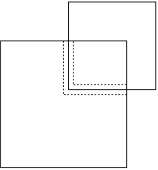
Figure 1. The larger cube is $P_{j}$, and the smaller cube is $Q_{i}$. The dashed line segments separate sets $P_{j,sep}$, $P_{j,\partial}$, and $\Delta_{P_{j}}$ from each other.

We write the matrix coefficient $\langle T\mathbf{1}_{P_{j}},\mathbf{1}_{Q_{i}}\rangle$ in (8.5) as

(8.7) $$\begin{split}&\langle T\mathbf{1}_{P_{j,\mathrm{sep}}},\mathbf{1}_{Q_{i}}\rangle+\langle T\mathbf{1}_{P_{j,\partial}},\mathbf{1}_{Q_{i}}\rangle+\langle T\mathbf{1}_{\Delta_{P_{j}}},\mathbf{1}_{\Delta_{Q_{i}}}\rangle+\langle T\mathbf{1}_{\Delta_{P_{j}}},\mathbf{1}_{Q_{i,\partial}}\rangle+\langle T\mathbf{1}_{\Delta_{P_{j}}},\mathbf{1}_{Q_{i,\mathrm{sep}}}\rangle\,,\end{split}$$

and these are denoted by $M_{1}(P)+M_{2}(P)+M_{3}(P)+M_{4}(P)+M_{5}(P)$, respectively.

8.2. Description of different terms

The heart of the argument lies in estimating terms

$$M_{3}(P)=\langle\mathbf{1}_{\Delta_{P_{j}}},T\mathbf{1}_{\Delta_{Q_{i}}}\rangle=\alpha_{1}(P)+\alpha_{2}(P)+\alpha_{3}(P),$$

where the last decomposition depends on a third random dyadic system $\mathcal{D}_{3}$, we refer to (8.9). Terms $\alpha_{2}(P)$ and $\alpha_{3}(P)$, along with $M_{2}(P)$ and $M_{4}(P)$, are ‘$\upsilon$-boundary’ terms. The ‘separated’ terms $M_{1}(P)$ and $M_{5}(P)$ are treated by kernel size condition.

The term $\alpha_{1}(P)$ will further be expanded in (8.10) as

$$\alpha_{1}(P)=\beta_{1}(P)+\beta_{2}(P)+\beta_{3}(P),$$

where $\beta_{1}(P)$ and $\beta_{2}(P)$ are so called ‘$\epsilon$-boundary’ terms. The local testing conditions and kernel size estimates are exploited in estimating ‘intersecting’ term $\beta_{3}(P)$.

8.3. Decomposition of $M_{3}(P)$

Without loss of generality, we can assume that $\Delta_{Q_{i}}\not=\emptyset$ and $\Delta_{P_{j}}\not=\emptyset$. Indeed, otherwise we already have $M_{3}(P)=0$.

We introduce a third random dyadic system $\mathcal{D}_{3}=\mathcal{D}(\omega_{3})$ that is independent of both $\mathcal{D}_{1}$ and $\mathcal{D}_{2}$. Fix $j(\upsilon)\in\mathrm{Z}$ such that $\upsilon/64\leq 2^{j(\upsilon)}<\upsilon/32$. Then, for every $P\in\mathcal{G}_{1}$ with $Q=Q(P)\not=\emptyset$, we define a layer

$$\mathcal{L}=\mathcal{L}(P,\upsilon):=\mathcal{D}_{3,\log_{2}(s)}$$

of $\mathcal{D}_{3}$-cubes with side length

(8.8) $$s=2^{j(\upsilon)}\ell Q_{i}=2^{j(\upsilon)}\cdot(\ell Q_{i}\wedge\ell P_{j})\,.$$

That is, $\mathcal{L}$ is a layer of $\mathcal{D}_{3}$ that depends on parameters $P$ and $\upsilon$.

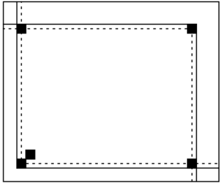
Figure 2. Parallelogram is $Q_{i}\cap P_{j}$. Interiors of some black $\mathcal{L}$-cubes intersect dashed line segments, which belong to the boundaries of either $\Delta_{P_{j}}$ or $\Delta_{Q_{i}}$. The $\mathcal{L}$-adjusted sets $\Delta_{Q_{i}}^{\mathcal{L}}$ and $\Delta_{P_{j}}^{\mathcal{L}}$, with solid boundaries, do not intersect the indicated $\mathcal{L}$-cubes.

Let $\Delta_{Q_{i}}^{\mathcal{L}},\Delta_{P_{j}}^{\mathcal{L}}\subset Q_{i}\cap P_{j}$ be the following adaptations of $\Delta_{Q_{i}}$ and $\Delta_{P_{j}}$ to $\mathcal{L}$. If necessary, we enlargen the latter sets so that, for every $G\in\mathcal{L}$, either $G\cap\Delta_{Q_{i}}^{\mathcal{L}}=G\cap\Delta_{P_{j}}^{\mathcal{L}}=G$ or one of the two intersections $G\cap\Delta_{Q_{i}}^{\mathcal{L}}$ and $G\cap\Delta_{P_{j}}^{\mathcal{L}}$ is empty. This is done in such a way that we can write

$$\Delta_{Q_{i}}^{\mathcal{L}}=\Delta_{Q_{i}}\cup\Delta^{\partial}_{Q_{i}}\,,\quad\Delta_{P_{j}}^{\mathcal{L}}=\Delta_{P_{j}}\cup\Delta^{\partial}_{P_{j}}\,,$$

both as disjoint unions, such that $\Delta^{\partial}_{Q_{i}}\subset Q_{i,\partial}\cap P_{j}$ and $\Delta^{\partial}_{P_{j}}\subset P_{j,\partial}\cap Q_{i}$. For an illustration, we refer to Figure 2.

Now observe that $M_{3}(P)=\langle T\mathbf{1}_{\Delta_{P_{j}}},\mathbf{1}_{\Delta_{Q_{i}}}\rangle$ can be written as

(8.9) $$\begin{split}\alpha_{1}(P)+\alpha_{2}(P)+\alpha_{3}(P)=\langle T\mathbf{1}_{\Delta_{P_{j}}^{\mathcal{L}}},\mathbf{1}_{\Delta_{Q_{i}}^{\mathcal{L}}}\rangle-\langle T\mathbf{1}_{\Delta_{P_{j}}^{\partial}},\mathbf{1}_{\Delta_{Q_{i}}^{\mathcal{L}}}\rangle-\langle T\mathbf{1}_{\Delta_{P_{j}}},\mathbf{1}_{\Delta_{Q_{i}}^{\partial}}\rangle\,.\end{split}$$

We remark that the terms in this decomposition depends on $\mathcal{D}_{3}$.

In order to define $\epsilon$-boundary terms, we let $P\in\mathcal{G}_{1}$ and write

$$L_{\epsilon}=L_{\epsilon}(P,\upsilon)=\bigcup_{G\in\mathcal{L}(P,\upsilon)}\delta_{G}^{\epsilon},\quad\delta_{G}^{\epsilon}=(1+\epsilon)G\setminus(1-\epsilon)G.$$

We also write $\widetilde{G}=G\setminus L_{\epsilon}$ if $G\in\mathcal{L}=\mathcal{L}(P,\upsilon)$. Define

$$\Delta^{\prime}_{Q_{i}}=\Delta^{\mathcal{L}}_{Q_{i}}\cap L_{\epsilon}\,,\quad\widetilde{\Delta}_{Q_{i}}=\Delta^{\mathcal{L}}_{Q_{i}}\setminus L_{\epsilon}\,,\quad\Delta^{\prime}_{P_{j}}=\Delta^{\mathcal{L}}_{P_{j}}\cap L_{\epsilon}\,,\quad\widetilde{\Delta}_{P_{j}}=\Delta^{\mathcal{L}}_{P_{j}}\setminus L_{\epsilon}\,.$$

Finally, we write $\alpha_{1}(P)=\langle T\mathbf{1}_{\Delta_{P_{j}}^{\mathcal{L}}},\mathbf{1}_{\Delta_{Q_{i}}^{\mathcal{L}}}\rangle$ as

(8.10) $$\begin{split}\beta_{1}(P)+\beta_{2}(P)+\beta_{3}(P)=\langle T\mathbf{1}_{\Delta^{\prime}_{P_{j}}},\mathbf{1}_{\Delta_{Q_{i}}^{\mathcal{L}}}\rangle+\langle T\mathbf{1}_{\widetilde{\Delta}_{P_{j}}},\mathbf{1}_{\Delta^{\prime}_{Q_{i}}}\rangle+\langle T\mathbf{1}_{\widetilde{\Delta}_{P_{j}}},\mathbf{1}_{\widetilde{\Delta}_{Q_{i}}}\rangle\,.\end{split}$$

9. The Nearby-Non-Boundary Term

We estimate summations involving the separated terms $M_{1}(P)$ and $M_{5}(P)$, and the intersecting term $\beta_{3}(P)$. All of the estimates will be uniform over all three dyadic grids.

9.1. Separated term

The two indicators appearing in either $M_{1}(P)$ or $M_{5}(P)$ are associated with sets separated from each other. This observation will allow us to prove inequality

(9.1) $$\bigg{|}\sum_{\begin{subarray}{c}P\in\mathcal{G}_{1}\end{subarray}}\langle\Delta_{P}f_{1}\rangle_{P_{j}}(M_{1}(P)+M_{5}(P))\langle\Delta_{Q}f_{2}\rangle_{Q_{i}}\bigg{|}\leq C(r,\upsilon)\,.$$

Proof of inequality (9.1).

We focus on summation over the terms $M_{1}(P)$, and the treatment of summation over terms $M_{5}(P)$ is analogous. We write $T_{P_{j},Q_{i}}=\mathbf{1}_{Q=Q(P)}\langle T\mathbf{1}_{P_{j,\mathrm{sep}}},\mathbf{1}_{Q_{i}}\rangle$. Then, by inequalities (8.1), the term under focus can be written as

$$\bigg{\lvert}\sum_{m=0}^{r}\sum_{u\in\{0,1\}}\sum_{k\in\mathbf{Z}}\sum_{\begin{subarray}{c}Q\in\mathcal{G}_{2,k-m}\end{subarray}}\sum_{\begin{subarray}{c}P\in\mathcal{G}_{1,k}\\ D(Q,P)/\ell P\sim 2^{u}\end{subarray}}\langle\Delta_{P}f_{1}\rangle_{P_{j}}T_{P_{j},Q_{i}}\langle\Delta_{Q}f_{2}\rangle_{Q_{i}}\bigg{\rvert}$$

$$\leq\sum_{m,u}\mathbf{A}_{m,u,i,j}\cdot\bigg{\lVert}\bigg{(}\sum_{k\in\mathbf{Z}}\sum_{Q\in\mathcal{G}_{2,k-m}}\lvert\Delta_{Q}f_{2}\rvert^{2}\bigg{)}^{1/2}\bigg{\rVert}_{p_{2}}\lesssim\sum_{m,u}\mathbf{A}_{m,u,i,j}\,,$$

where we have denoted

$$\mathbf{A}_{m,u,i,j}=\bigg{\lVert}\bigg{(}\sum_{k\in\mathbf{Z}}\sum_{Q\in\mathcal{G}_{2,k-m}}\bigg{\lvert}\mathbf{1}_{Q_{i}}\sum_{\begin{subarray}{c}P\in\mathcal{G}_{1,k}\\ D(Q,P)/\ell P\sim 2^{u}\end{subarray}}\langle\Delta_{P}f_{1}\rangle_{P_{j}}\frac{T_{P_{j},Q_{i}}}{\mu(Q_{i})}\bigg{\rvert}^{2}\bigg{)}^{1/2}\bigg{\rVert}_{p_{1}}\,.$$

The proof of inequality (9.1) is finished by invoking Lemma 9.2 below. ∎

9.2 Lemma.

For $m\in\{0,1,\ldots,r\}$ and $u\in\{0,1\}$, we have $\rvert\mathbf{A}_{m,u,i,j}\lvert\leq C(r,\upsilon)$.

Proof.

For each $k\in\mathbf{Z}$ and $S\in\mathcal{D}_{1,k+u+\theta(u+m)}$, define a kernel

(9.3) $$K_{S}(x,y)=\sum_{\begin{subarray}{c}P\in\mathcal{G}_{1,k}\\ P\subset S\end{subarray}}\sum_{\begin{subarray}{c}Q\in\mathcal{G}_{2,k-m}\\ D(Q,P)/\ell P\sim 2^{u}\end{subarray}}\mathbf{1}_{Q_{i}}(x)\cdot\widetilde{T}_{P_{j},Q_{i}}\cdot\mathbf{1}_{P_{j}}(y)\,,\qquad x,y\in\mathbf{R}^{n}\,,$$

where $\widetilde{T}_{P_{j},Q_{i}}=\mathbf{1}_{Q=Q(P)}\widetilde{T}_{P_{j},Q_{i}}$ is defined by

$$\frac{T_{P_{j},Q_{i}}}{\mu(P_{j})\mu(Q_{i})}=\frac{\widetilde{T}_{P_{j},Q_{i}}}{\mu(S)}\,.$$

Consider cubes $P$ and $Q$ as in the definition of $K_{S}$, and let $y\in P_{j,\textup{sep}}$ and $x\in Q_{i}$. By the upper doubling properties of $\mu$, and the facts that $\lvert x-y\rvert\geq\upsilon 2^{-r}\ell P_{j}$ and $S\subset B(y,2^{1+u+\theta(u+m)}\ell P)$, we find that $\lambda(y,\lvert x-y\rvert)^{-1}\leq C(r,\upsilon)\mu(S)^{-1}$. Hence, by definition,

$$\lvert T_{P_{j},Q_{i}}\rvert\leq\int_{Q_{i}}\int_{P_{j,\textup{sep}}}\frac{1}{\lambda(y,\lvert x-y\rvert)}\,d\mu(y)\,d\mu(x)\leq C(r,\upsilon)\mu(Q_{i})\mu(P_{j})\mu(S)^{-1}\,.$$

As a consequence $\lvert\widetilde{T}_{P_{j},Q_{i}}\rvert\leq C(r,\upsilon)$ and, by recalling Lemma 2.12,

(9.4) $$\begin{split}\lvert K_{S}(x,y)\rvert&\leq C(r,\upsilon)\sum_{\begin{subarray}{c}P\in\mathcal{G}_{1,k}\\ P\subset S\end{subarray}}\sum_{\begin{subarray}{c}P\in\mathcal{G}_{2,k-m}\\ D(Q,P)/\ell P\sim 2^{u}\end{subarray}}\mathbf{1}_{Q_{i}}(x)\cdot\mathbf{1}_{P_{j}}(y)\leq C(r,\upsilon)\cdot\mathbf{1}_{S}(x)\cdot\mathbf{1}_{S}(y)\,.\end{split}$$

After these preparations, we finish the proof by proceeding as in Lemma 7.2. ∎

9.2. Intersecting term

The following inequality deals with intersecting part, i.e., terms $\beta_{3}(P)$;

(9.5) $$\bigg{|}\sum_{\begin{subarray}{c}P\in\mathcal{G}_{1}\end{subarray}}\langle\Delta_{P}f_{1}\rangle_{P_{j}}\beta_{3}(P)\langle\Delta_{Q}f_{2}\rangle_{Q_{i}}\bigg{|}\leq C(r,\upsilon,\epsilon)(1+\mathbf{T}_{\textup{loc}})\,.$$

The proof of this inequality relies on the kernel size estimate and local testing conditions.

Proof of inequality (9.5).

We tacitly restrict all the summations here to cubes $P\in\mathcal{G}_{1}$ for which $\mu(Q_{i}\cap P_{j})\not=0$. Indeed, otherwise $\beta_{3}(P)=0$. By writing $\mu(Q_{i}\cap P_{j})=\int\mathbf{1}_{Q_{i}}\mathbf{1}_{P_{j}}\,d\mu$ and using Cauchy-Schwarz and Hölder’s inequality,

(9.6) $$\begin{split}&\bigg{|}\sum_{P\in\mathcal{G}_{1}}\langle\Delta_{P}f_{1}\rangle_{P_{j}}\beta_{3}(P)\langle\Delta_{Q}f_{2}\rangle_{Q_{i}}\bigg{|}\\ &\leq\bigg{\|}\bigg{(}\sum_{P\in\mathcal{G}_{1}}\lvert\langle\Delta_{P}f_{1}\rangle_{P_{j}}\mathbf{1}_{P_{j}}\rvert^{2}\bigg{)}^{1/2}\bigg{\|}_{p_{1}}\cdot\bigg{\|}\bigg{(}\sum_{P\in\mathcal{G}_{1}}\bigg{\lvert}\frac{\beta_{3}(P)}{\mu(Q_{i}\cap P_{j})}\langle\Delta_{Q}f_{2}\rangle_{Q_{i}}\mathbf{1}_{Q_{i}}\bigg{\rvert}^{2}\bigg{)}^{1/2}\bigg{\|}_{p_{2}}.\end{split}$$

By inequality (2.6), the first factor is bounded by $\lesssim 1$. Let us then focus on the second factor; by writing the summation in terms of $Q$ and using Lemma (9.7), we obtain an upper bound $C(r,\upsilon,\epsilon)(1+\mathbf{T}_{\textup{loc}})$ for the second term. ∎

9.7 Lemma.

Let $P\in\mathcal{G}_{1}$. Then $|\beta_{3}(P)|\leq C(r,\upsilon,\epsilon)(1+\mathbf{T}_{\textup{loc}})\mu(Q_{i}\cap P_{j})$.

Proof.

We can assume that $Q=Q(P)\not=\emptyset$, hence $P\sim Q$. Consider the expansion,

$$\beta_{3}(P)=\langle T\mathbf{1}_{\widetilde{\Delta}_{P_{j}}},\mathbf{1}_{\widetilde{\Delta}_{Q_{i}}}\rangle=\sum_{\begin{subarray}{c}G,H\in\mathcal{L}\\ G\not=H\end{subarray}}\langle T(\mathbf{1}_{G}\mathbf{1}_{\widetilde{\Delta}_{P_{j}}}),\mathbf{1}_{H}\mathbf{1}_{\widetilde{\Delta}_{Q_{i}}}\rangle+\sum_{G\in\mathcal{L}}\langle T(\mathbf{1}_{G}\mathbf{1}_{\widetilde{\Delta}_{P_{j}}}),\mathbf{1}_{G}\mathbf{1}_{\widetilde{\Delta}_{Q_{i}}}\rangle.$$

In both of the series above, the finite number of summands depends on $n$ and $\upsilon$. Hence, it suffices to obtain estimates for individual summands for fixed $G,H\in\mathcal{L}$. First, if $G\not=H$, then

$$\ell Q_{i}\leq C(r,\upsilon,\epsilon)\,\mathrm{dist}(G\cap\widetilde{\Delta}_{P_{j}},H\cap\widetilde{\Delta}_{Q_{i}}).$$

In particular, $\lambda(x,\lvert x-y\rvert)^{-1}\leq C(r,\upsilon,\epsilon)\mu(Q_{i})^{-1}$ if $x\in H\cap\widetilde{\Delta}_{Q_{i}}$ and $y\in G\cap\widetilde{\Delta}_{P_{j}}$. Hence,

(9.8) $$\begin{split}|\langle T(\mathbf{1}_{G}\mathbf{1}_{\widetilde{\Delta}_{P_{j}}}),\mathbf{1}_{H}\mathbf{1}_{\widetilde{\Delta}_{Q_{i}}}\rangle|&\leq\int_{H\cap\widetilde{\Delta}_{Q_{i}}}\int_{G\cap\widetilde{\Delta}_{P_{j}}}\frac{1}{\lambda(x,\lvert x-y\rvert)}\,d\mu(y)\,d\mu(x)\\ &\leq C(r,\upsilon,\epsilon)\frac{\mu(Q_{i}\cap P_{j})\mu(Q_{i}\cap P_{j})}{\mu(Q_{i})}\leq C(r,\upsilon,\epsilon)\mu(Q_{i}\cap P_{j}).\end{split}$$

In the last step, we also used the fact that $\widetilde{\Delta}_{P_{j}}\cup\widetilde{\Delta}_{Q_{i}}\subset Q_{i}\cap P_{j}$.

Then we consider the case of $G=H$. By construction,

(9.9) $$\langle T(\mathbf{1}_{G}\mathbf{1}_{\widetilde{\Delta}_{P_{j}}}),\mathbf{1}_{G}\mathbf{1}_{\widetilde{\Delta}_{Q_{i}}}\rangle=\begin{cases}\langle T\mathbf{1}_{\widetilde{G}},\mathbf{1}_{\widetilde{G}}\rangle,\quad&\text{if }G=G\cap\Delta_{P_{j}}^{\mathcal{L}}=G\cap\Delta_{Q_{i}}^{\mathcal{L}}\,;\\ 0&\text{otherwise}.\end{cases}$$

In any case, by local testing conditions $\lvert\langle T(\mathbf{1}_{G}\mathbf{1}_{\widetilde{\Delta}_{P_{j}}}),\mathbf{1}_{G}\mathbf{1}_{\widetilde{\Delta}_{Q_{i}}}\rangle\rvert\leq\mathbf{T}_{\textup{loc}}\mu(\widetilde{G})\leq\mathbf{T}_{\textup{loc}}\mu(Q_{i}\cap P_{j})$. ∎

10. The Nearby-Boundary Term

Here we treat the $\epsilon$ and $\upsilon$ boundary terms by probabilistic arguments.

10.1. The $\epsilon$-boundary terms

Following inequality controls summation for $\epsilon$-boundary terms. Let $t>p_{1}\vee p_{2}$ be a positive real number. Then

(10.1) $$\mathbf{E}_{\omega_{3}}\bigg{|}\sum_{\begin{subarray}{c}P\in\mathcal{G}_{1}\end{subarray}}\langle\Delta_{P}f_{1}\rangle_{P_{j}}\big{(}\beta_{1}(P)+\beta_{2}(P)\big{)}\langle\Delta_{Q}f_{2}\rangle_{Q_{i}}\bigg{|}\leq C(r,\upsilon)\epsilon^{1/t}\mathbf{T}\,.$$

The expectations over the dyadic system $\mathcal{D}_{3}$ are crucial here, and here only.

We let $\epsilon=(\varepsilon_{k})_{k\in\mathbf{Z}}$ be a sequence of Rademacher variables, supported on a probability space $(\Omega,\mathbf{P})$. We can also associate Rademacher variables to $\mathcal{D}_{j}$-dyadic cubes with $j\in\{1,2\}$:— fix an injection $R\mapsto j(R):\mathcal{D}_{j}\to\mathbf{Z}$, and use notation $\varepsilon_{R}=\varepsilon_{j(R)}$.

We rely on the following improvement of the contraction principle, [MR2491037, Lemma 3.1].

10.2 Proposition.

Suppose that $\{\rho_{k}\,:\,k\in\mathbf{Z}\}\subset L^{t}(\widetilde{\Omega})$ for some $\sigma$-finite measure space $(\widetilde{\Omega},\widetilde{\mathbf{P}})$ and $t\in(2,\infty)$. Then, for all complex-valued sequences $(\xi_{k})_{k\in\mathbf{Z}}$,

$$\bigg{\|}\sum_{k=-\infty}^{\infty}\varepsilon_{k}\rho_{k}\xi_{k}\bigg{\|}_{L^{t}(\widetilde{\Omega};L^{2}(\Omega))}\lesssim\sup_{k\in\mathbf{Z}}\|\rho_{k}\|_{L^{t}(\widetilde{\Omega})}\cdot\bigg{\|}\sum_{k=-\infty}^{\infty}\varepsilon_{k}\xi_{k}\bigg{\|}_{L^{2}(\Omega)}\,.$$

Proof of inequality (10.1).

Let us focus on the sum involving the terms $\beta_{1}(P)$; the estimate for the sum involving terms $\beta_{2}(P)$ is similar. We randomize and use Hölder’s inequality,

(10.3) $$\begin{split}&\bigg{|}\sum_{\begin{subarray}{c}P\in\mathcal{G}_{1}\end{subarray}}\langle\Delta_{P}f_{1}\rangle_{P_{j}}\langle T\mathbf{1}_{\Delta^{\prime}_{P_{j}}},\mathbf{1}_{\Delta_{Q_{i}}^{\mathcal{L}}}\rangle\langle\Delta_{Q}f_{2}\rangle_{Q_{i}}\bigg{|}\\ &=\bigg{|}\int_{\Omega}\Big{\langle}T\Big{(}\sum_{S\in\mathcal{G}_{1}}\varepsilon_{S}\mathbf{1}_{\Delta^{\prime}_{S_{j}}}\langle\Delta_{S}f_{1}\rangle_{S_{j}}\Big{)},\sum_{P\in\mathcal{G}_{1}}\varepsilon_{P}\mathbf{1}_{\Delta_{Q_{i}}^{\mathcal{L}}}\langle\Delta_{Q}f_{2}\rangle_{Q_{i}}\Big{\rangle}d\mathbf{P}(\epsilon)\bigg{|}\\ &\leq\bigg{\lVert}T\Big{(}\sum_{S\in\mathcal{G}_{1}}\varepsilon_{S}\mathbf{1}_{\Delta^{\prime}_{S_{j}}}\langle\Delta_{S}f_{1}\rangle_{S_{j}}\Big{)}\bigg{\|}_{L^{p_{1}}(\Omega\times\mathbf{R}^{n})}\bigg{\|}\sum_{P\in\mathcal{G}_{1}}\varepsilon_{P}\mathbf{1}_{\Delta_{Q_{i}}^{\mathcal{L}}}\langle\Delta_{Q}f_{2}\rangle_{Q_{i}}\bigg{\rVert}_{L^{p_{2}}(\Omega\times\mathbf{R}^{n})}.\end{split}$$

Index the very last summation in terms of $\mathcal{D}_{2}$. This can be done by using our standing assumptions of $P\mapsto Q(P)=Q$. Then, by the contraction principle and inequality $|\mathbf{1}_{\Delta_{Q_{i}}^{\mathcal{L}}}|\leq\mathbf{1}_{Q_{i}}$, we see that the second factor in the last line of (10.3) is bounded (up to a constant multiple) by $\lVert f_{2}\rVert_{p_{2}}\lesssim 1$.

In order to estimate the first factor in the last line of (10.3) we first extract operator norm $\mathbf{T}$. Then we fix $S\in\mathcal{G}_{1,k}$ with $k\in\mathrm{Z}$. By (8.1) and (8.8),

$$\Delta_{S_{j}}^{\prime}\subset L_{\epsilon}(S,\upsilon)=\bigcup_{G\in\mathcal{L}(S,\upsilon)}\delta_{G}^{\epsilon}\subset\bigcup_{m=j(\upsilon)+k-r-1}^{j(\upsilon)+k-1}\bigcup_{G\in\mathcal{D}_{3,m}}\delta^{\varepsilon}_{G}=:\delta^{\epsilon}(k).$$

Hence, we have $\mathbf{1}_{\Delta^{\prime}_{S_{j}}}\leq\mathbf{1}_{\delta^{\epsilon}(k)}\mathbf{1}_{S_{j}}$. By the contraction principle and assumption $t\geq p_{1}$,

(10.4) $$\begin{split}&\mathbf{E}_{\omega_{3}}\bigg{\|}\sum_{S\in\mathcal{G}_{1}}\varepsilon_{S}\mathbf{1}_{\Delta^{\prime}_{S_{j}}}\langle\Delta_{S}f_{1}\rangle_{S_{j}}\bigg{\|}_{L^{p_{1}}(\Omega\times\mathbf{R}^{n})}\lesssim\mathbf{E}_{\omega_{3}}\bigg{\|}\sum_{k\in\mathrm{Z}}\varepsilon_{k}\mathbf{1}_{\delta^{\epsilon}(k)}\sum_{S\in\mathcal{D}_{1,k}}\mathbf{1}_{S_{j}}\langle\Delta_{S}f_{1}\rangle_{S_{j}}\bigg{\|}_{L^{p_{1}}(\Omega\times\mathbf{R}^{n})}\\ &\quad\leq\bigg{(}\int_{\mathbf{R}^{n}}\bigg{[}\mathbf{E}_{\omega_{3}}\bigg{\|}\sum_{k\in\mathrm{Z}}\varepsilon_{k}\mathbf{1}_{\delta^{\epsilon}(k)}(x)\sum_{S\in\mathcal{D}_{1,k}}\mathbf{1}_{S_{j}}(x)\langle\Delta_{S}f_{1}\rangle_{S_{j}}\bigg{\|}^{t}_{L^{p_{1}}(\mathbf{\Omega})}\bigg{]}^{p_{1}/t}d\mu(x)\bigg{)}^{1/p_{1}}.\end{split}$$

For a fixed $x\in\mathbf{R}^{n}$, the last integrand evaluated at $x$ is of the form as in Proposition 10.2 with $\xi_{k}=\sum_{S\in\mathcal{D}_{1,k}}\mathbf{1}_{S_{j}}(x)\langle\Delta_{S}f_{1}\rangle_{S_{j}}$. Moreover, the random variables $\rho_{k}:=\mathbf{1}_{\delta^{\epsilon}(k)}(x)$ as functions of $\omega_{3}\in\Omega_{3}=(\{0,1\}^{n})^{\mathbf{Z}}$ belong to $L^{t}(\Omega_{3})$, and they satisfy

$$\sup_{k\in\mathrm{Z}}\|\mathbf{1}_{\delta^{\epsilon}(k)}(x)\|_{L^{t}(\Omega_{3})}=\sup_{k\in\mathrm{Z}}\mathbf{P}_{\omega_{3}}(\mathbf{1}_{\delta^{\epsilon}(k)}(x)=1)^{1/t}\leq C(r,\upsilon)\epsilon^{1/t}.$$

Hence, by Proposition 10.2 and Khintchine’s inequality,

$$LHS\eqref{e.crc}\leq C(r,\upsilon)\epsilon^{1/t}\bigg{\|}\sum_{S\in\mathcal{D}_{1}}\varepsilon_{S}\mathbf{1}_{S_{j}}\langle\Delta_{S}f_{1}\rangle_{S_{j}}\bigg{\|}_{L^{p_{1}}(\Omega\times\mathbf{R}^{n})}\leq C(r,\upsilon)\epsilon^{1/t}\,.$$

The proof is complete. ∎

10.2. The $\upsilon$-boundary terms

The following inequality controls summation of the $\upsilon$-boundary terms. Let $t>p_{1}\vee p_{2}$. Then

(10.5) $$\mathbf{E}_{\omega_{1}}\mathbf{E}_{\omega_{2}}\bigg{|}\sum_{\begin{subarray}{c}P\in\mathcal{G}_{1}\end{subarray}}\langle\Delta_{P}f_{1}\rangle_{P_{j}}(M_{2}(P)+M_{4}(P)+\alpha_{2}(P)+\alpha_{3}(P))\langle\Delta_{Q}f_{2}\rangle_{Q_{i}}\bigg{|}\leq C(r)\upsilon^{1/t}\mathbf{T}\,.$$

Before the proof, let us remark that although both $\alpha_{2}(P)$ and $\alpha_{3}(P)$ depend on the random dyadic system $\mathcal{D}_{3}$, the inequality is uniform over all such systems.

Proof of inequality (10.5).

First we observe that functions $f_{j}$ depend on both dyadic systems, as they are (essentially) projections to good cubes. This dependency is not allowed in the argument below. Fortunately, this issue can be easily addressed—if $Q(P)\not=\emptyset$ in the series above, we have both $P\in\mathcal{G}_{1}$ and $Q=Q(P)\in\mathcal{G}_{2}$. Then, in particular $\Delta_{P}f_{1}=\Delta_{P}\widetilde{f_{1}}$ and $\Delta_{Q}f_{2}=\Delta_{Q}\widetilde{f}_{2}$. Functions $\widetilde{f}_{j}$ do not depend on the dyadic systems, and we use them to replace $f_{j}$’s.

By (8.7) and (8.9), $M_{2}(P)+\alpha_{2}(P)$ and $M_{4}(P)+\alpha_{3}(P)$ are given by

$$\langle T\mathbf{1}_{P_{j,\partial}},\mathbf{1}_{Q_{i}}\rangle-\langle T\mathbf{1}_{\Delta_{P_{j}}^{\partial}},\mathbf{1}_{\Delta_{Q_{i}}^{\mathcal{L}}}\rangle;\quad\langle T\mathbf{1}_{\Delta_{P_{j}}},\mathbf{1}_{Q_{i,\partial}}\rangle-\langle T\mathbf{1}_{\Delta_{P_{j}}},\mathbf{1}_{\Delta_{Q_{i}}^{\partial}}\rangle\,,$$

respectively. Observe that

(10.6) $$\begin{split}&(\mathbf{1}_{P_{j,\partial}}+\mathbf{1}_{\Delta_{P_{j}}^{\partial}})\lesssim\mathbf{1}_{P_{j,\partial}},\quad(\mathbf{1}_{Q_{i}}+\mathbf{1}_{\Delta_{Q_{i}}^{\mathcal{L}}})\lesssim\mathbf{1}_{Q_{i}}\,,\quad\mathbf{1}_{\Delta_{P_{j}}}\lesssim\mathbf{1}_{P_{j}},\,\,\,\quad(\mathbf{1}_{Q_{i,\partial}}+\mathbf{1}_{\Delta_{Q_{i}}^{\partial}})\lesssim\mathbf{1}_{Q_{i,\partial}}.\end{split}$$

pointwise $\mu$-almost everywhere. By triangle inequality, it suffices to estimate the following sums: one involving terms $m(P)\in\{M_{2}(P),\alpha_{2}(P)\}$, and the other involving terms in $\{M_{4}(P),\alpha_{3}(P)\}$. We focus on the first sum; the second one is estimated in an analogous manner, using $\mathbf{E}_{\omega_{1}}$.

By randomizing, using Hölder’s inequality, extracting the operator norm of $T$, and applying the contraction principle with inequalities (10.6),

(10.7) $$\begin{split}&\mathbf{E}_{\omega_{2}}\bigg{|}\sum_{\begin{subarray}{c}P\in\mathcal{G}_{1}\end{subarray}}\langle\Delta_{P}\widetilde{f}_{1}\rangle_{P_{j}}m(P)\langle\Delta_{Q}\widetilde{f}_{2}\rangle_{Q_{i}}\bigg{|}\\ &\lesssim\mathbf{T}\cdot\mathbf{E}_{\omega_{2}}\bigg{\{}\bigg{\|}\sum_{S\in\mathcal{G}_{1}}\varepsilon_{S}\mathbf{1}_{S_{j,\partial}}\langle\Delta_{P}\widetilde{f}_{1}\rangle_{S_{j}}\bigg{\|}_{L^{p_{1}}(\Omega\times\mathbf{R}^{n})}\bigg{\|}\sum_{Q\in\mathcal{D}_{2}}\varepsilon_{Q}\mathbf{1}_{Q_{i}}\langle\Delta_{Q}\widetilde{f}_{2}\rangle_{Q_{i}}\bigg{\|}_{L^{p_{2}}(\Omega\times\mathbf{R}^{n})}\bigg{\}}.\end{split}$$

By the contraction principle, we find that the last factor is $\omega_{2}$-uniformly bounded by $\lesssim\lVert\widetilde{f}_{2}\rVert_{p_{2}}=1$. In order to treat the remaining factor, we write

$$\delta^{\upsilon}(k)=\bigcup_{m=k-r-1}^{k-1}\bigcup_{Q\in\mathcal{D}_{2,m}}\delta^{\upsilon}_{Q}.$$

By (8.1) and (8.6), $\mathbf{1}_{S_{j,\partial}}\leq\mathbf{1}_{S_{j}}\mathbf{1}_{\delta_{Q_{i}}^{\upsilon}}\leq\mathbf{1}_{S_{j}}\mathbf{1}_{\delta^{\upsilon}(k)}$ if $Q=Q(S)$ with $S\in\mathcal{G}_{1,k}$. Fix $x\in\mathbf{R}^{n}$. The random variables $\rho_{k}:=\mathbf{1}_{\delta^{\upsilon}(k)}(x)$ as functions of $\omega_{2}\in(\{0,1\}^{n})^{\mathrm{Z}}$ belong to $L^{t}((\{0,1\}^{n})^{\mathrm{Z}})$,

$$\sup_{k\in\mathrm{Z}}\|\mathbf{1}_{\delta^{\upsilon}(k)}(x)\|_{L^{t}((\{0,1\}^{n})^{\mathrm{Z}})}=\sup_{k\in\mathrm{Z}}\mathbf{P}_{\omega_{2}}(\mathbf{1}_{\delta^{\upsilon}(k)}(x)=1)^{1/t}\leq C(r)\upsilon^{1/t}.$$

Hence, proceeding as in connection with (10.4), we find that

$$\mathbf{E}_{\omega_{2}}\bigg{\|}\sum_{S\in\mathcal{G}_{1}}\varepsilon_{S}\mathbf{1}_{S_{j,\partial}}\langle\Delta_{P}\widetilde{f}_{1}\rangle_{S_{j}}\bigg{\|}_{L^{p_{1}}(\Omega\times\mathbf{R}^{n})}\leq C(r)\upsilon^{1/t}\bigg{\|}\sum_{P\in\mathcal{D}_{1}}\varepsilon_{P}\mathbf{1}_{P_{j}}\langle\Delta_{P}\widetilde{f}_{1}\rangle_{P_{j}}\bigg{\|}_{L^{p_{1}}(\Omega\times\mathbf{R}^{n})}.$$

The last term is bounded by a constant multiple of $C(r)\upsilon^{1/t}$. ∎

• refs