and

A simple and fast algorithm for computing exponentials of power series

Abstract

As was initially shown by Brent, exponentials of truncated power series can be computed using a constant number of polynomial multiplications. This note gives a relatively simple algorithm with a low constant factor.

3 March 2009

Let $\mathbb{K}$ be a ring of characteristic zero and let $h$ be in $\mathbb{K}[[x]]$ with $h(0)=0$. The exponential of $h$ is the power series

$$\exp(h)=\sum_{i\geq 0}\frac{h^{i}}{i!}.$$

Computing exponentials is useful for many purposes, such as solving differential equations [4] or recovering a polynomial from the power sums of its roots [11].

Using Newton iteration, it has been known since Brent’s work [3] that exponentials could be computed for the cost of polynomial multiplication, up to a constant factor. Following this original result, a series of works aimed at lowering the multiplicative factor; they all rely on some form of Newton iteration, either of order 2 (the “usual” form of iteration) or of higher order. Remark that the question of improving constant factors can be asked with other applications of Newton iteration (power series inversion, square root, …) [12, 2, 6], but we do not discuss those here.

As is customary, we assume that the base ring $\mathbb{K}$ supports the Fast Fourier Transform (as an aside, note that in the Karatsuba multiplication model, exponential computation has an asymptotic cost equivalent to that of multiplication [7, § 4.2.2]). If $m\in\mathbb{N}$ is any power of $2$, we suppose that $\mathbb{K}$ contains a $m$th primitive root of unity $\omega_{m}$ such that in addition $\omega_{m}=\omega_{2m}^{2}$; also, 2 is a unit in $\mathbb{K}$. We denote by $\mathsf{E}(m)$ an upper bound on the cost of evaluating a polynomial of degree less than $m$ at the points $(1,\omega_{m},\dots,\omega_{m}^{m-1}).$ Using Fast Fourier Transform, we have $\mathsf{E}(m)\in O(m\log m)$; we also ask that $\mathsf{E}$ satisfies the super-linearity property $\mathsf{E}(2m)\geq 2\mathsf{E}(m)$.

Theorem 1

Let $h\in\mathbb{K}[[x]]$, with $h(0)=0$ and let $n\in\mathbb{N}$ be a power of $2$. Then, starting from $\omega_{n}$ and from the first $n$ coefficients of $h$, one can compute the first $n$ coefficients of $\exp(h)$ using $16\frac{1}{2}\mathsf{E}(n)+24\frac{1}{4}n$ operations in $\mathbb{K}$.

Using Fast Fourier Transform, polynomials of degree less than $n$ can be multiplied in $3\mathsf{E}(2n)+O(n)$ operations. Hence, we say that an exponential can be computed for (essentially) the cost of $2\frac{3}{4}$ multiplications. References to previous work given below use the same ratio “cost of exponential vs. cost of multiplication”.

As documented by Bernstein [1], the initial algorithm by Brent had cost $7\frac{1}{3}$ times that of multiplication. Bernstein successively reduced the constant factor to $3\frac{4}{9}$ and $2\frac{5}{6}$ [2] using high-order iterations. Recently, van der Hoeven [10] obtained an even better constant of $2\frac{1}{3}$. However, that algorithm (using a high-order iteration) is quite complex (to wit, the second-order term in the cost estimate is likely not linear in $n$); we are not aware of an existing implementation of it.

As to order-2 iterations, Bernstein [2] obtained a constant of $3\frac{1}{3}$, which was superseded by Hanrot and Zimmermann’s $3\frac{1}{4}$ result [6]. The merits of our algorithm is thus to be a simple yet faster second order iteration. Compared to van der Hoeven’s result, we are asymptotically slower, but we could expect to be better for a significant range of $n$, due to the simplicity of our algorithm.

Proof.

For $a=\sum_{i\geq 0}a_{i}x^{i}\in\mathbb{K}[[x]]$, we write $a\bmod x^{\ell}=\sum_{i=0}^{\ell-1}a_{i}x^{i}$ and $a{\rm~{}div~{}}x^{\ell}=\sum_{i\geq 0}a_{i+\ell}x^{i}$; computing these quantities does not require any arithmetic operation. In Figure 1, we first give the standard iteration (left), taken from Hanrot and Zimmermann’s note [6], followed by an expanded version where polynomial multiplications are isolated (right). Correctness of the left-hand version is proved in [6]; in particular, each time we enter the loop at Step 2, $f=\exp(h)\bmod x^{m}$ and $g=1/f\bmod x^{m/2}$ hold.

Exp$(h,n)$
1.	$f=1,g=1,m=1$
2.	while $m\leq n/2$ do
2.a		$g=(2g-fg^{2})\bmod x^{m}$
2.b		$q=h^{\prime}\bmod x^{m-1}$
2.c		$w=q+g(f^{\prime}-fq)\bmod x^{2m-1}$
2.d		$f=f+f(h-\int w)\bmod x^{2m}$
2.e		$m=2m$
3.	return $f$

Exp$(h,n)$
1′.	$f=1,g=1,m=1$
2′.	while $m\leq n/2$ do
2.a′		$g=(2g-fg^{2})\bmod x^{m}$
2.b′		$q=h^{\prime}\bmod x^{m-1}$
2.c′		$r=fq\bmod(x^{m}-1)$
2.d′		$s=x(f^{\prime}-r)\bmod(x^{m}-1)$
2.e′		$t=gs\bmod x^{m}$
2.f′		$u=(h\bmod x^{2m}-\int tx^{m-1}){\rm~{}div~{}}x^{m}$
2.g′		$v=fu\bmod x^{m}$
2.h′		$f=f+x^{m}v$
2.i′		$m=2m$
3′.	return $f$

Figure 1: Two versions of the exponential computation

To prove the correctness of our version, it is enough to show that it computes the same output as the original one. When entering Step 2 we have $f=\exp(h)\bmod x^{m}$; it follows that $x(f^{\prime}-qf)=0\bmod x^{m}$, with $q=h^{\prime}\bmod x^{m-1}$. Since $x(f^{\prime}-qf)$ has degree less than $2m$, we deduce that the quantity $s$ of Step 2.d^′ satisfies $x(f^{\prime}-qf)=x^{m}s$. This implies that $t=gs\bmod x^{m}$ satisfies $tx^{m-1}=g(f^{\prime}-qf)\bmod x^{2m-1}$, so that the quantities $w$ of Step 2.c and $u$ of Step 2.f^′ satisfy $u=((h-\int w)\bmod x^{2m}){\rm~{}div~{}}x^{m}$. The original iteration satisfies $h-\int w=0\bmod x^{m}$, so that actually $x^{m}u=(h-\int w)\bmod x^{2m}$ and thus $x^{m}v=f(h-\int w)\bmod x^{2m}$, with $v=fu\bmod x^{m}$. The correctness claim follows.

For $f$ in $\mathbb{K}[x]$ and $m$ a power of 2, we define

$$\text{{DFT}}(f,m)=(f(1),\dots,f(\omega_{m}^{m-1})),\quad\text{{DFT}}^{\prime}(f,m)=(f(\omega_{2m}),\dots,f(\omega_{2m}\omega_{m}^{m-1})),$$

so that $\text{{DFT}}(f,2m)$ is, up to reordering, the concatenation of $\text{{DFT}}(f,m)$ and $\text{{DFT}}^{\prime}(f,m)$. Recall that if $f$ has degree less than $m$, then $\text{{DFT}}(f,m)$ can be computed in time $\mathsf{E}(m)$; besides, $\text{{DFT}}^{\prime}(f,m)$ can be computed in time $\mathsf{E}(m)+2m$ (due to the scaling by $\omega_{2m}$); the inverse DFT in length $m$ can be performed in time $\mathsf{E}(m)+m$ (due to $m$ divisions by $m$).

With this, we finally analyze the cost of the algorithm step by step. We assume that the $n$ elements $(1,\omega_{n},\dots,\omega_{n}^{n-1})$ have been precomputed in time $n$ once and for all, and stored, so that they are freely available during the remaining computations. The hypothesis $\omega_{m}=\omega_{2m}^{2}$ ensures that all the needed DFT’s solely use (part of) these $n$ elements.

In what follows, we assume $m$ is a power of $2$, with $m\geq 2$, so that $m/2$ is an integer. Recall that at the input of Step 2, $f$ has degree at most $m-1$ and $g$ has degree at most $m/2-1$; additionally, we suppose that $\text{{DFT}}(g,m)$ is known. Then, the key ingredients are as follows:

1. We will compute $\text{{DFT}}(g,2m)$; since $\text{{DFT}}(g,m)$ is already known, it is enough to compute $\text{{DFT}}^{\prime}(g,m)$, which saves a factor of 2.

2. Since $x(f^{\prime}-qf)=x^{m}s$, we can compute it modulo $x^{m}-1$.

Step 2.a^′

This step updates $g$ to $1/f\bmod x^{m}$. The product $fg^{2}$ has degree less than $2m$; it is computed by FFT multiplication in length $2m$. Since $\text{{DFT}}(g,m)$ is known, we do not need to compute $\text{{DFT}}(g,2m)$ but only $\text{{DFT}}^{\prime}(g,m)$. Hence, the cost is $\mathsf{E}(2m)\text{\ (DFT of $f$)}+\mathsf{E}(m)+m\text{\ (DFT${}^{\prime}$ of $g$)}+4m\text{\ (pairwise products)}+\mathsf{E}(2m)+2m\text{\ (inverse DFT)}$.

By the fundamental property of Newton iteration, the first $m/2-1$ coefficients of $g$ and $2g-fg^{2}$ coincide. Hence, to deduce $2g-fg^{2}\bmod x^{m}$, only $m/2$ sign changes are needed.

Step 2.b^′

Differentiation takes time $m$; since half of the coefficients were computed at the previous loop, the cost can be reduced to $m/2$.

Step 2.c^′

We compute $r$ by FFT multiplication in length $m$. Since $\text{{DFT}}(f,2m)$, and thus $\text{{DFT}}(f,m)$, is known, the cost is $2\mathsf{E}(m)+2m$.

Step 2.d^′

Computing $f^{\prime}-r$ takes time $2m$; multiplication by $x$ modulo $x^{m}-1$ is free.

Step 2.e^′

The product $gs$ has degree less than $2m$; it is computed by FFT multiplication in length $2m$, of cost $3\mathsf{E}(2m)+4m$. This provides $\text{{DFT}}(g,2m)$, which will be used as input in the next iteration.

Step 2.f^′

Integration and subtraction together take time $2m$.

Step 2.g^′

The product $fu$ has degree less than $2m$; it is computed by FFT multiplication in length $2m$. Since $\text{{DFT}}(f,2m)$ is known, the cost is $2\mathsf{E}(2m)+4m$.

Step 2.h^′

This step is free.

Hence, the cost of one pass through the main loop is at most $3\mathsf{E}(m)+7\mathsf{E}(2m)+22m$. At the last iteration, with $m=n/2$, savings are possible at Step 2.e^′, since we do not need to precompute $\text{{DFT}}(g,2m)$ for the next iteration. To compute $t=gs\bmod x^{m}$, we write

$$g=g_{0}+x^{m/2}g_{1},\quad s=s_{0}+x^{m/2}s_{1},\quad t=g_{0}s_{0}+x^{m/2}(g_{0}s_{1}+g_{1}s_{0})\bmod x^{m}.$$

We compute $g_{0}s_{0}$ and $g_{0}s_{1}+g_{1}s_{0}$ by FFT’s of order $m$. Since $\text{{DFT}}(g_{0},m)$ is known, we just need to compute $\text{{DFT}}(g_{1},m)$, $\text{{DFT}}(s_{0},m)$ and $\text{{DFT}}(s_{1},m)$, as well as 2 inverse DFT’s, for a cost of $5\mathsf{E}(m)+2m$; the other linear costs (inner products and additions) sum up to $4\frac{1}{2}m$. Adding all costs gives the claimed complexity result in Theorem 1.

The case of arbitrary $n$.

We gave our algorithm for $n$ a power of $2$ (the algorithm of [6] does not have this restriction, but assumes that Fourier transforms can be performed at arbitrary lengths $n$). We describe here possible workarounds for the general case.

For an arbitrary value of $n$, Newton iteration will compute the approximations $\exp(h)\bmod x^{m_{i}}$, where the sequence $(m_{i})_{i\geq 0}$ is defined by $r=\lceil\log_{2}(n)\rceil$ and $m_{i}=\lceil n/2^{r-i}\rceil$, as in [5, Ex. 9.6], so that $m_{i}$ is either $2m_{i-1}$ or $2m_{i-1}-1$ and thus $m_{i-1}=\lceil m_{i}/2\rceil$. Then, the algorithm enters Step 2 knowing $f=\exp(h)\bmod x^{m_{i}}$ and $g=1/f\bmod x^{m_{i-1}}$; it exits Step 2 with $f=\exp(h)\bmod x^{m_{i+1}}$ and $g=1/f\bmod x^{m_{i}}$. Depending on the Fourier Transform model we use, our improvements can be carried over to this case as well.

In a model which allows Fourier transforms at roots of unity of any order, our algorithm extends in a rather straightforward manner. As before, we also suppose that $\text{{DFT}}(g,m_{i})$ is known at the beginning of Step 2, where now DFT can be taken at arbitrary order. Now, the multiplications at Steps 2.a^′, 2.c^′ and 2.g^′ are done with transforms of order respectively $2m_{i}$, $m_{i}$ and $2m_{i}$, but that of Step 2.c^′ has order $m_{i+1}$ to enable the next iteration. This gives $\exp(h)\bmod x^{2m_{i}}$, and thus $\exp(h)\bmod x^{m_{i+1}}$, by truncating off the last coefficient in the case where $m_{i+1}=2m_{i}-1$.

In a model where only roots of unity of order $2^{k}$ are allowed, it is possible to use van der Hoeven’s Truncated Fourier Transform [8]. For $f\in\mathbb{K}[x]$ of degree less than $m$, let $\text{{TFT}}(f,m)$ denote the values $(f(w^{[0]_{r}}),\dots,f(\omega^{[i_{m-1}]_{r}}))$, where $r=\lceil\log_{2}(m)\rceil$, $\omega$ is a primitive root of unity of order $2^{r}$, and $[i]_{r}$ is the bitwise mirror of $i$ in length $r$.

A first difficulty is that the relationship between $\text{{TFT}}(f,m)$ and $\text{{TFT}}(f,2m)$ is less transparent than in the case of the classical Fourier transform. Step 2.a^′ requires to compute only the values $\text{{TFT}}(f,2m)-\text{{TFT}}(f,m)$; while it is obviously possible to adapt van der Hoeven’s algorithm to this case, as in [9, § 5], determining the exact cost requires a specific study. A second issue is that using the values $\text{{TFT}}(f,m)$ does not allow immediately to perform multiplication modulo $x^{m}-1$, which is needed to compute $s$ at Step 2.d^′ of our algorithm. However, this problem can be solved by computing $s/x^{m}$, which is a polynomial of degree less than $m$ (remark that the same issue arises if one wants to use the Truncated Fourier Transform in the algorithm of [6]).

Experiments.

Figure 2 gives empirical results, using the FFT routines for small Fourier primes implemented in Shoup’s NTL library [13]. As can be seen, a ratio close to the expected 2.75 is observed.

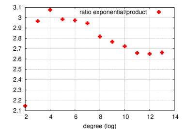
Figure 2: Ratio exponential vs. product

References

- [1] D. J. Bernstein. http://cr.yp.to/fastnewton.html.
- [2] D. J. Bernstein. Removing redundancy in high-precision Newton iteration, 2004. Available at http://cr.yp.to/fastnewton.html.
- [3] R. P. Brent. Multiple-precision zero-finding methods and the complexity of elementary function evaluation. In Analytic computational complexity, pages 151–176. Academic Press, 1976.
- [4] R. P. Brent and H. T. Kung. Fast algorithms for manipulating formal power series. Journal of the ACM, 25(4):581–595, 1978.
- [5] J. von zur Gathen and J. Gerhard. Modern computer algebra. Cambridge University Press, 1999.
- [6] G. Hanrot and P. Zimmermann. Newton iteration revisited. Available at http://www.loria.fr/~zimmerma/papers.
- [7] J. van der Hoeven. Relax, but don’t be too lazy. J. Symb. Comput., 34(6):479–542, 2002.
- [8] J. van der Hoeven. The Truncated Fourier Transform and applications. In ISSAC’04, pages 290–296. ACM, 2004.
- [9] J. van der Hoeven. Notes on the Truncated Fourier Transform. Technical Report 2005-5, Université Paris-Sud, 2005. Available at http://www.math.u-psud.fr/~vdhoeven/.
- [10] J. van der Hoeven. Newton’s method and FFT trading. Technical Report 2006-17, Université Paris-Sud, 2006. Available at http://www.math.u-psud.fr/~vdhoeven/.
- [11] A. Schönhage. The fundamental theorem of algebra in terms of computational complexity, 1982. Preprint Univ. Tübingen.
- [12] A. Schönhage. Variations on computing reciprocals of power series. Inform. Process. Lett., 74:41–46, 2000.
- [13] V. Shoup. NTL: A library for doing number theory. Available at http://www.shoup.net.