Abstract

Magnetization dynamics in the system of magnetic nanoclusters with randomly distributed properties are studied by means of computer simulations. The main attention is paid to the possibility of coherent magnetization reversal from a strongly nonequilibrium state with a mean cluster magnetization directed opposite to an external magnetic field. Magnetic nanoclusters are known to be characterized by large magnetic anisotropy and strong dipole interactions. It is also impossible to produce a number of nanoclusters with identical properties. As a result, any realistic system of nanoclusters is composed of the clusters with randomly varying anisotropies, effective spins, and dipole interactions. Despite this randomness, it is possible to find conditions when the cluster spins move coherently and display fast magnetization reversal due to the feedback action of resonator. By analyzing the influence of different cluster parameters, we find their optimal values providing fast magnetization reversal.

PACS: 75.75.Jn; 75.78.Cd; 76.20.+q; 76.90.+d

Keywords: magnetic nanoclusters, magnetization dynamics, magnetization reversal

^∗Corresponding author: V.I. Yukalov (E-mail: yukalov@theor.jinr.ru)

1 Introduction

Magnetic nanoclusters are the objects enjoying rich and interesting properties with a variety of applications, as can be inferred form the review articles [1, 2, 3, 4, 5]. For example, they are used in magnetic chemistry as catalysts; in biomedical imaging for magnetic reading by magnetometers that measure the magnetic field change induced by nanoclusters; in medical treatment by employing alternating magnetic fields forcing the oscillation of the nanocluster magnetic moment that produces heat destroying ill cells or bacteria; in genetic engineering by attaching a nanocluster to a particular piece of the molecule and then removing it together with this piece; in waste cleaning by stacking nanoclusters to waste and then removing them together with waste; in information storage, processing, and quantum computing; and so on [1, 2, 3, 4, 5]. This is why the methods of governing magnetization dynamics of nanoclusters are so much important.

The use of nano sizes of clusters is principal, since such clusters behave as large monodomain particles with a given large total spin. Typical radii of nanoclusters are between 1 and 100 nm, containing from 100 to $10^{5}$ atoms. Respectively, the effective total magnetization of a cluster can be of order 100 to $10^{5}\mu_{B}$. The maximal size of a cluster, when it is in a monodomain state, such that the spins of atoms, composing the cluster, sum up coherently, forming an effective total spin, is characterized by the coherence radius. The clusters, whose sizes are larger than the coherence radius, decompose into several domains with oppositely directed magnetization, so that the total cluster spin is zero.

Employing nanoclusters for the purpose of information storage, processing, and quantum computing meets the requirements that contradict each other. From one side, for information storage, it is required that the cluster magnetization could be well frozen in a given direction, which needs the existence of a sufficiently large magnetic anisotropy. But, from another side, for information processing, it is necessary to be able to quickly reverse the cluster magnetization, which is hindered by this anisotropy.

Nanoclusters enjoy the property to get their magnetization frozen at temperatures lower than the blocking temperature that is of order of 10 - 100 K. Then to reverse the cluster magnetization, one has to overcome the magnetic anisotropy. So, for information storage, one needs large magnetic anisotropy, while for information processing, the anisotropy has to be suppressed to achieve fast magnetization reversal. To accomplish such a reversal, one applies external transverse fields pushing the cluster magnetization. The discussion of different methods of magnetization reversal by means of external magnetic fields can be found in Refs. [2, 3, 4, 5, 6].

A very efficient method for realizing fast magnetization reversal of nanoclusters is based on the use of feedback field from a resonant electric circuit coupled to the ensemble of nanoclusters [6, 7, 8, 9, 10]. Actually, the idea that a resonant electric circuit can drastically shorten the relaxation time of a spin system was advanced by Purcell [11], who illustrated it for an ensemble of nuclear spins. This mechanism has later been considered by Blombergen and Pound [12]. The influence of the coupling of a magnetic sample with a resonant circuit on magnetization dynamics is called the Purcell effect. One sometimes calls it the radiation damping, following Bloembergen and Pound [12]. However the latter term is rather a misnomer, as has been stressed by a number of researchers [13, 14, 15], since the coupling of a spin system with a resonator does strongly influences spin dynamics, but not necessarily damping it. For instance, this effect enhances nuclear magnetic resonance signals, which is widely used in NMR techniques [16, 17, 18]. The term ”radiation damping” is also confusing because of making impression that these are spins themselves that cooperate by interacting with each other through a common radiation field. Such a radiation correlation between radiating atoms is the essence of the Dicke effect [19]. But for magnetic particles, as has already been stressed by Purcell [11], such a radiation collectivization of spin motion is absolutely negligible. In atomic physics, one clearly distinguishes these two principally different physical effects. And the term Purcell effect is employed for describing the influence of a cavity resonator on atomic radiation, which is the main part of the cavity quantum electrodynamics [20, 21, 22].

The role of the Purcell effect on the spin dynamics of nuclear spins is well studied. In resonance experiments, it enhances the NMR signals [16, 17, 18]. For strongly nonequilibrium systems of polarized nuclei, it leads to fast magnetization reversal [23, 24, 25, 26, 27] that has been discovered in experiments [23] and later confirmed in other experimental studies (see references in the review article [4]).

Magnetization dynamics in an ensemble of nanoclusters is essentially different from that of nuclear systems. The basic differences are as follows.

(i) Nanoclusters possess rather large magnetic anisotropy that hinders the possibility of simple regulation of spin motion.

(ii) Having large effective spins, nanoclusters also have strong spin dipole interactions, which results in short dephasing time.

(iii) The most important difficulty for organizing collective spin motion in a system of nanoclusters is the problem of cluster inhomogeneity, since nanoclusters, being prepared by any of the known methods, whether by thermal decomposition, or microemulsion reactions, or by thermal spraying, are not identical particles, as nuclei would be. But nanoclusters differ by their shapes and sizes, which results in the difference in the value of their spins, dipole interactions, and of their anisotropies.

It is the aim of the present paper to investigate the magnetization dynamics in a realistic inhomogeneous ensemble of nanoclusters exhibiting all their typical properties of anisotropy and dipole interactions. Since analytic investigation of such an inhomogeneous system is too much complicated, we resort to computer modelling. Because the problem of magnetization reversal is of special interest for many applications, such as information recording and processing, we pay the main attention to finding the optimal conditions, when the magnetization reversal is fast and as close to complete as possible.

2 Realistic model of nanocluster system

The sample formed by a system of nanoclusters is described by the Hamiltonian

$$\hat{H}=\sum_{i}\hat{H}_{i}+\frac{1}{2}\sum_{i\neq j}\hat{H}_{ij}\;,$$ (1)

where the first term characterizes single nanoclusters and the second term describes their dipole interactions.

The typical Hamiltonian of a nanocluster has the form

$$\hat{H}_{i}=-\mu_{i}{\bf B}\cdot{\bf S}_{i}-D(S_{i}^{z})^{2}+D_{2}(S_{i}^{y})^{2}+D_{4}\left[(S_{i}^{x})^{2}(S_{i}^{y})^{2}+(S_{i}^{y})^{2}(S_{i}^{z})^{2}+(S_{i}^{z})^{2}(S_{i}^{x})^{2}\right]\;,$$ (2)

in which the first term is the Zeeman energy, and other terms describe the energy due to magnetic anisotropy, with the corresponding anisotropy parameters [1, 2, 3, 4, 5, 6].

The interaction Hamiltonian is caused by dipole spin interactions

$$\hat{H}_{ij}=\sum_{\alpha\beta}D_{ij}^{\alpha\beta}S_{i}^{\alpha}S_{j}^{\beta}\;,$$ (3)

with the dipolar tensor

$$D_{ij}^{\alpha\beta}=\frac{\mu_{0}^{2}}{r_{ij}^{3}}\left(\delta_{\alpha\beta}-3n_{ij}^{\alpha}n_{ij}^{\beta}\right)\;,$$ (4)

where

$$r_{ij}\equiv|{\bf r}_{ij}|\;,\qquad{\bf n}_{ij}\equiv\frac{{\bf r}_{ij}}{r_{ij}}\;,\qquad{\bf r}_{ij}\equiv{\bf r}_{i}-{\bf r}_{j}\;.$$

The total magnetic field, acting on the system, is the sum

$${\bf B}=B_{0}{\bf e}_{z}+H{\bf e}_{x}$$ (5)

of an external constant field $B_{0}$ and the resonator feedback field $H$.

The considered sample is inserted into a coil of an electric circuit with an attenuation $\gamma$ and natural frequency $\omega$. Moving spins of the sample create electric current in the coil that, in turn, produces the feedback magnetic field acting on these spins. The equation for the feedback field follows from the Kirchhoff equation and can be written [4, 26, 27] as

$$\frac{dH}{dt}+2\gamma H+\omega^{2}\int_{0}^{t}H(t^{\prime})\;dt^{\prime}=-4\pi\eta\;\frac{dm_{x}}{dt}\;,$$ (6)

where $\eta$ is filling factor and the electromotive force is caused by the moving average magnetization density

$$m_{x}=\frac{\mu_{0}}{V}\sum_{j}\langle S_{j}^{x}\rangle\;.$$ (7)

The equations of spin dynamics are obtained in the following traditional way [4, 14, 28, 29]. First, we write the Heisenberg equations of motion for the spin components $S_{j}^{\alpha}$, in which the index $j=1,2,\ldots,N$ enumerates nanoclusters and $\alpha=x,y,z$. Then these equations are averaged using semiclassical approximation, and spin attenuation is taken into account by means of the second-order perturbation theory, as is described in full details by Abragam and Goldman [14, 29]. This procedure results in the equations that can effectively be obtained from the evolution equations

$$i\hbar\;\frac{d}{dt}\;S_{j}^{x}=[S_{j}^{x},H]-i\Gamma_{2}S_{j}^{x}\;,$$

$$i\hbar\;\frac{d}{dt}\;S_{j}^{y}=[S_{j}^{y},H]-i\Gamma_{2}S_{j}^{y}\;,$$

$$i\hbar\;\frac{d}{dt}\;S_{j}^{z}=[S_{j}^{z},H]-i\gamma_{1}\left(S_{j}^{z}-S\right)\;,$$ (8)

with the straightforward use of the semiclassical approximation [4, 14, 28, 29]. Here $\Gamma_{2}$ is a transverse attenuation parameter, $\gamma_{1}$ is longitudinal attenuation parameter, and $S\equiv\sum_{j=1}^{N}S_{j}/N$ is average spin value. In the case of strong initial polarization, the transverse attenuation is characterized [4, 14, 27, 29] by the expression

$$\Gamma_{2}=\gamma_{2}(1-s^{2})\;,$$ (9)

where $s$ is the reduced average spin

$$s\equiv\frac{1}{N}\sum_{j=1}^{N}\frac{\langle S_{j}^{z}\rangle}{S_{j}}\;,$$ (10)

and the natural width is

$$\gamma_{2}\equiv\frac{\rho\mu_{0}^{2}S}{\hbar}=\rho\hbar\gamma_{S}^{2}S\;.$$ (11)

In the following numerical calculations, we shall use the reduced dimensionless attenuation parameters, measured in units of the Zeeman frequency

$$\omega_{0}\equiv-\;\frac{\mu_{0}B_{0}}{\hbar}=|\gamma_{S}|B_{0}\;,\qquad(\mu_{0}=-2\mu_{B}=-\hbar|\gamma_{S}|)\;.$$ (12)

Our goal is to investigate spin dynamics of nanoclusters with realistic parameters. Thus, the values of the anisotropy parameters, typical for nanoclusters, such as Co, Fe, and Ni nanoclusters, are

$$\frac{D}{\hbar\gamma_{2}}=10^{-3}\;,\qquad\frac{D_{2}}{\hbar\gamma_{2}}=10^{-3}\;,\qquad\frac{D_{4}}{\hbar\gamma_{2}}=10^{-10}\;.$$ (13)

Studying spin dynamics, we shall take into account that real nanoclusters are not completely identical with each other, but exhibit the dispersion in their anisotropy parameters and spin values. The main aim of our study is to analyze how the parameter dispersion influences spin dynamics and to find conditions allowing for effective spin reversal.

3 Introduction of dimensionless system parameters

For numerical analysis, it is convenient to pass to dimensionless quantities. To this end, we define the dimensionless resonator feedback field

$$p_{H}\equiv\frac{H}{B_{0}}$$ (14)

and the reduced transverse attenuation, caused by dipole interactions,

$$p_{d}\equiv\frac{\gamma_{2}}{\omega_{0}}\;.$$ (15)

Also, we introduce the dimensionless anisotropy parameters

$$p_{A}\equiv\frac{\omega_{A}}{\omega_{0}}\;,\qquad p_{B}\equiv\frac{\omega_{B}}{\omega_{0}}\;,\qquad p_{C}\equiv\frac{\omega_{C}}{\omega_{0}}\;,$$ (16)

expressed through the anisotropy frequencies

$$\omega_{A}\equiv 2S\;\frac{D}{\hbar}\;,\qquad\omega_{B}\equiv 2S\;\frac{D_{2}}{\hbar}\;,\qquad\omega_{C}\equiv 2S^{3}\;\frac{D_{4}}{\hbar}\;.$$ (17)

In the equations of motion, we employ the reduced spin, with the components

$$e_{\alpha}\equiv\frac{1}{N}\;\sum_{j=1}^{N}\;\frac{S_{j}^{\alpha}}{S_{j}}\;,\qquad e_{z}\equiv s\;.$$ (18)

Since the nanocluster spins $S_{j}$ are large, of order $10^{3}$, the semiclassical approximation is well justified. This allows us to treat $\bf{e}$ as a classical vector. The evolution will be considered with respect to the dimensionless time

$$\widetilde{t}\equiv\omega_{0}t\;.$$ (19)

At the initial moment of time, there is no feedback field, which assumes the initial conditions

$$p_{H}(0)=0\;,\qquad\dot{p}_{H}(0)=0\;,$$ (20)

where the overdot implies time derivative.

The initial conditions for the spin polarization $e_{z}(0)$ are constructed as follows [30, 31]. For the given value of an initial polarization $e_{z}(0)$, a variety of the initial orientations for the individual vectors $S_{j}^{z}(0)$ are admissible. These orientations can be prescribed by a kind of Monte Carlo techniques. First, a random configuration of vectors $S_{j}^{z}$ is taken and the corresponding total polarization is evaluated. A new direction is chosen randomly for each spin, and the new total polarization is calculated. If it is less than the initial one, the array with the changed magnetic moment direction distribution is chosen as the second iteration, otherwise, it is rejected. This procedure is repeated until the system achieves the required average polarization $e_{z}(0)$ playing the role of the initial condition. The initial spin polarization is assumed to be directed opposite to the external magnetic field $B_{0}$.

4 Optimal conditions for spin reversal

We accomplish numerical solution of the evolution equations for $N=15^{3}=3375$ spins, searching for the conditions of the optimal spin reversal. The Zeeman frequency $\omega_{0}$ is taken to be in resonance with the circuit natural frequency $\omega$.

The peculiarity of spin reversal depends on the system parameters. For instance, the optimal value of the resonator attenuation $\gamma$, defined by the resonator circuit quality, essentially depends on the given transverse attenuation $\gamma_{2}$, caused by spin dipole interactions.

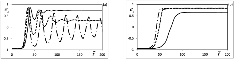
Figure 1: Dynamics of the average spin polarization $e_{z}=s$, for the ratio $\gamma_{2}/\omega_{0}=0.01$, as a function of dimensionless time, for random spins with the mean $S=1200$ and relative spin variance $\delta S/S=0.333$ for different values of the resonator attenuation: (a) $\gamma/\omega_{0}=0$ (dashed-dotted line), $\gamma/\omega_{0}=0.04$ (dashed line), $\gamma/\omega_{0}=0.12$ (solid line); (b) $\gamma/\omega_{0}=0.3$ (dashed-dotted line), $\gamma/\omega_{0}=0.4$ (dashed line), $\gamma/\omega_{0}=0.8$ (solid line).

Let us fix $\gamma_{2}=0.01\omega_{0}$, which yields $p_{d}=0.01$, and let us take the anisotropy parameters typical for Co, Fe, and Ni nanoclusters, as defined above. Below the blocking temperature, the longitudinal relaxation is suppressed, so that $\gamma_{1}$ is much smaller than $\gamma_{2}$, which allows us to set $\gamma_{1}/\gamma_{2}=10^{-3}$. The coil filling factor is assumed to be close to one. The nanocluster spins are randomly distributed by the normal law with mean $S=1200$ and variance $\delta S=400$. Dynamics of spin polarization, $e_{z}$, is shown in Fig. 1 for different resonator attenuations $\gamma$. Varying $\gamma$, we are looking for its optimal value that provides the maximal permanent reversal, without superimposed oscillations. It is this regime that is optimal for fast and stable information processing [32]. As is seen, for the given ratio $\gamma_{2}/\omega_{0}$, the optimal value of the resonator attenuation is $\gamma\approx 0.35\omega_{0}$. Below this value, the reversal is slower and the reversed spin value is smaller. For very low $\gamma$, there is no reversal at all. Above the optimal value of $\gamma$, there arise oscillations, and the reversed spin value diminishes.

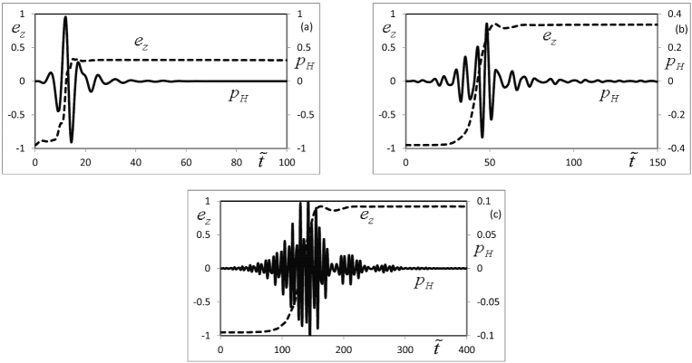
Figure 2: Average spin polarization $e_{z}=s$ (dashed line) and feedback field $p_{H}$ (solid line) as functions of dimensionless time, for different ratios $p_{d}=\gamma_{2}/\omega_{0}$, with the corresponding optimal $\gamma$: (a) $p_{d}=0.1,\gamma/\omega_{0}=0.7$; (b) $p_{d}=0.01,\gamma/\omega_{0}=0.3$; (c) $p_{d}=0.001,\gamma/\omega_{0}=0.1$. Spins are randomly distributed as in Fig.1.

The spin reversal is caused by the resonator feedback field. This is illustrated in Fig. 2, where it is seen that the reversal occurs when the amplitude of the feedback-field oscillations is maximal and almost reaches the strength of the external field $B_{0}$. For each given ratio $p_{d}=\gamma_{2}/\omega_{0}$, the corresponding optimal value of $\gamma$ is chosen. The stronger external field $B_{0}$, that is, the larger $\omega_{0}$, hence, smaller $p_{d}$, the more effective is the reversal, though the reversal time increases. Spin magnitudes are randomly distributed, as in Fig. 1.

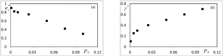
Figure 3: Dependence of the optimal $\gamma^{*}$ and the related value of the reversed spin $s^{*}=e_{z}^{*}$, as functions of the ratio $p_{d}=\gamma_{2}/\omega_{0}$.

The dependence of the optimal $\gamma^{*}$ and the related value of the reversed spin $s^{*}=e_{z}^{*}$, as functions of the ratio $p_{d}=\gamma_{2}/\omega_{0}$, are presented in Fig. 3. The larger the ratio $p_{d}$, the larger the optimal $\gamma^{*}$, but the smaller the value of the reversed spin $s^{*}$.

In addition to spin dispersion, there can exist the dispersion of the anisotropy parameters. We study spin dynamics, when the spins as well as all anisotropy parameters are distributed by the normal law. The spin mean is taken as $S=1200$ and variance as $\delta S=960$. The mean values of the anisotropy parameters are assumed to be typical for the Co, Fe, and Ni nanoclusters, as in Eq. (13), with the relative variance

$$\frac{\delta D}{D}=\frac{\delta D_{2}}{D_{2}}=\frac{\delta D_{4}}{D_{4}}=0.1\;.$$

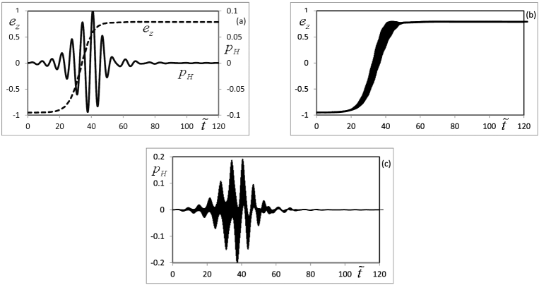
Figure 4: Influence of the combined dispersion of spins and anisotropy parameters on the dynamics of spin reversal for $p_{d}=\gamma_{2}/\omega_{0}=0.01$, with the corresponding optimal $\gamma/\omega_{0}=0.3$: (a) spin polarization $s=e_{z}$ (dashed line) and feedback field $p_{H}$ (solid line) as functions of the dimensionless time for random spins with the relative spin variance $\delta S/S=0.8$ and fixed anisotropy parameters; (b) Spin polarization $s=e_{z}$, averaged over 30 realizations of the anisotropy distribution with the relative variance 0.1, as a function of the dimensionless time; (c) feedback field $p_{H}$ as a function of the dimensionless time, averaged over 30 realizations of the anisotropy distribution.

We accomplish 30 realizations of spin dynamics varying the anisotropy parameters, with random spin distribution in each of the realizations. The results, averaged over the realizations, are shown in Fig. 4. We see that a rather strong dispersion of the system parameters does not preclude spin reversal.

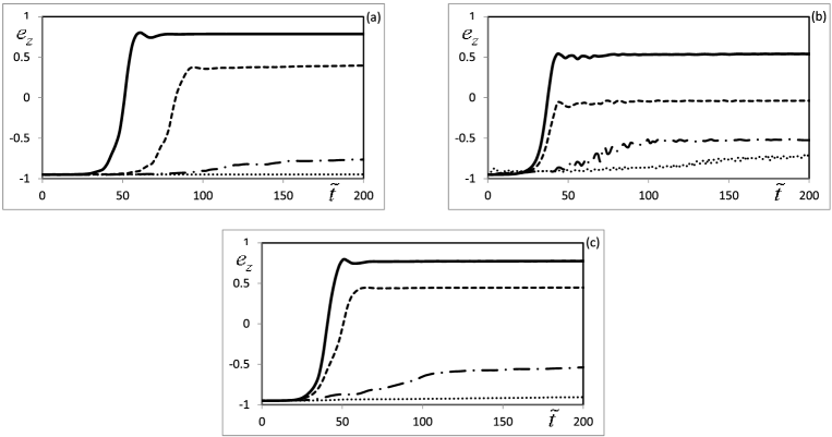
Figure 5: Spin polarization $s=e_{z}$, as a function of dimensionless time, for the ratio $p_{d}=\gamma_{2}/\omega_{0}=0.01$, with the corresponding optimal $\gamma/\omega_{0}=0.3$, for varying anisotropy parameters: (a) $p_{A}=0.1$ (solid line), $p_{A}=0.2$ (dashed line), $p_{A}=0.3$ (dashed-dotted line), $p_{A}=0.4$ (dotted line); (b) $p_{B}=0.5$ (solid line), $p_{B}=1$ (dashed line), $p_{B}=2$ (dashed-dotted line), $p_{B}=3$ (dotted line); (c) $p_{C}=0.1$ (solid line), $p_{C}=0.2$ (dashed line), $p_{C}=0.3$ (dashed-dotted line), $p_{C}=0.4$ (dotted line). In each case, spins are randomly distributed with mean 1200 and relative variance 0.3.

To understand when the spin reversal could be blocked by anisotropy, we vary the parameters of the latter in a wide range, looking for the values at which the reversal becomes blocked. Varying one of the anisotropy parameters, we keep others fixed. Spins are randomly distributed with mean $S=1200$ and relative variance 0.3. Fig. 5 illustrates the results, from which the blocking anisotropy parameters are evaluated as

$$\frac{D}{\hbar\gamma_{2}}\sim 10^{-2}\;,\qquad\frac{D_{2}}{\hbar\gamma_{2}}\sim 0.5\times 10^{-1}\;,\qquad\frac{D_{4}}{\hbar\gamma_{2}}\sim 10^{-8}\;.$$

These blocking parameters are essentially larger than the typical values in Eq. (13). Hence, the typical anisotropy does not block spin reversal.

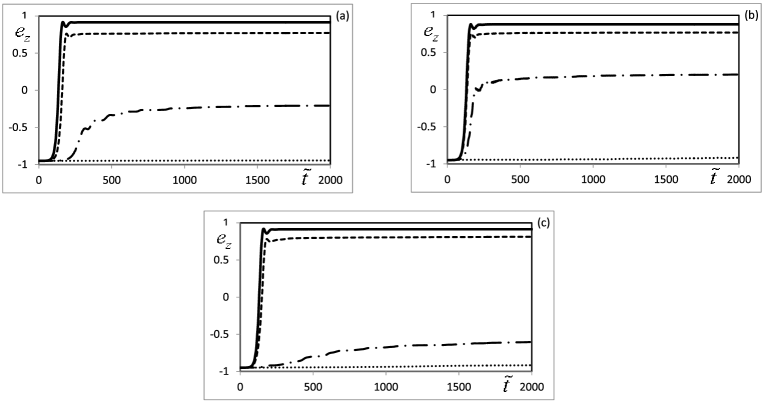
Figure 6: Spin polarization $s=e_{z}$, as a function of dimensionless time, for the ratio $p_{d}=\gamma_{2}/\omega_{0}=0.01$, with the corresponding optimal $\gamma/\omega_{0}=0.3$, for varying anisotropy parameters: (a) $p_{A}=0.01$ (solid line), $p_{A}=0.05$ (dashed line), $p_{A}=0.1$ (dashed-dotted line), $p_{A}=0.2$ (dotted line); (b) $p_{B}=0.05$ (solid line), $p_{B}=0.1$ (dashed line), $p_{B}=0.2$ (dashed-dotted line), $p_{B}=0.5$ (dotted line); (c) $p_{C}=0.01$ (solid line), $p_{C}=0.05$ (dashed line), $p_{C}=0.1$ (dashed-dotted line), $p_{C}=0.2$ (dotted line). In each case, spins are randomly distributed with mean 1200 and relative variance 0.3.

With increasing external field $B_{0}$, that is, diminishing the ratio $p_{d}=\gamma_{2}/\omega_{0}$, the blocking anisotropy parameters decrease. This is illustrated by Fig. 6 that is to be compared with Fig. 5. So, increasing the external field suppresses the role of the anisotropy.

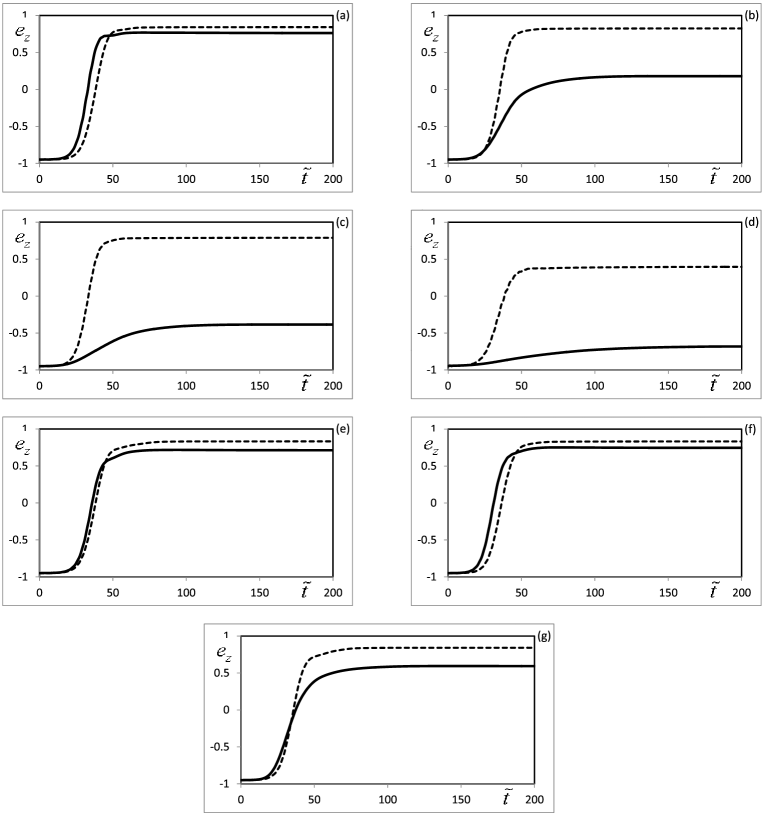
Figure 7: Spin polarization $s=e_{z}$, as a function of dimensionless time, for the ratio $p_{d}=\gamma_{2}/\omega_{0}=0.01$, with the related optimal $\gamma/\omega_{0}=0.3$, for varying anisotropy parameters. Solid line describes the case of strong spin dispersion, with mean spin $S=1200$ and relative variance $\delta S/S=1$. Dashed line corresponds to the case without spin dispersion. The anisotropy parameters are: (a) $p_{A}=0.01$, $p_{B}=0.01$, $p_{C}=0.001$, (b) $p_{A}=0.05$, $p_{B}=0.1$, $p_{C}=0.05$, (c) $p_{A}=0.1$, $p_{B}=0.2$, $p_{C}=0.1$, (d) $p_{A}=0.2$, $p_{B}=0.7$, $p_{C}=0.2$, (e) $p_{A}=0.05$, $p_{B}=0.01$, $p_{C}=0.001$, (f) $p_{A}=0.01$, $p_{B}=0.1$, $p_{C}=0.001$, (g) $p_{A}=0.01$, $p_{B}=0.01$, $p_{C}=0.02$.

Finally, we study whether a strong spin dispersion can destroy the coherent spin dynamics and influence spin reversal. For this purpose, we consider a random distribution of spins, with mean $S=1200$ and very large relative variance $\delta S/S=1$. The results of numerical simulations are given in Fig. 7 for the ratio $p_{d}=\gamma_{2}/\omega_{0}=0.01$, with the corresponding optimal $\gamma/\omega_{0}=0.3$, and varying anisotropy parameters. The results demonstrate that, for small anisotropy parameters, spin dispersion plays practically no role. This role increases for larger values of the anisotropy parameters. This fact finds straightforward explanation from the structure of the spin equations of motion. When the anisotropy parameters are much smaller than the Zeeman frequency, the spin rotation is governed by the same $\omega_{0}$ depending only on the external field $B_{0}$, but independent of the spin lengths. But when the anisotropy parameters are sufficiently large, approaching their blocking values, then the anisotropy disturbs the effective rotation frequencies, so that different spins rotate with different frequencies. This is equivalent to the appearance of inhomogeneous broadening. Fortunately, the typical nanocluster anisotropy parameters are much lower than their blocking values. So, for a sufficiently strong external field, all spins rotate with almost the same frequency $\omega_{0}$ and their dispersion even being quite large, does not much influence their motion. Then the coherent spin dynamics can be realized, resulting in a fast spin reversal.

5 Conclusion

We have studied the magnetization dynamics in an ensemble of magnetic nanoclusters, keeping in mind a realistic situation, when the nanoclusters are characterized by a microscopic Hamiltonian, with well defined parameters. Another peculiarity of realistic nanocluster ensembles is the dispersion in the values of their spins and anisotropy parameters, which we also take into account. We have accomplished a series of computer simulations varying the system properties and searching for the conditions when the magnetization reversal is optimal, in the sense of being fast, maximal, and quasi-stationary, without oscillations. Such a process of magnetization reversal is necessary in a variety of applications. For instance, for realizing effective quantum information processing.

For numerical values, we have chosen the nanocluster parameters typical for Co, Fe, and Ni nanoclusters. It turns out that if the external magnetic field defines the Zeeman frequency that is essentially larger than the effective anisotropy frequencies, then the dispersion of spin magnitudes plays practically no role. This also concerns the dispersion in the values of the anisotropy parameters. The external magnetic field, sufficient for this effect is 1 T, which corresponds to the Zeeman frequency $\omega_{0}\sim 10^{11}$ Hz.

We have shown that the magnetization reversal is caused by the resonator feedback field that is self-organized by moving spins. The value of the feedback field, in the moment of spin reversal, almost reaches the value of the external field. Fast magnetization reversal can be achieved solely by moving spins themselves, without involving strong transverse magnetic fields. For such nanoclusters as Co, Fe, and Ni, the reversal time can be of order $10^{-11}$ s. This conclusion suggests a convenient mechanism for the efficient manipulation of nanocluster magnetization, which is of high importance for a variety of applications.

Acknowledgment

The authors acknowledge financial support from the Russian Foundation for Basic Research under the projects 10-02-96023, 11-02-00086, 11-07-96007, and 12-02-00897. One of the authors (V.I.Y.) is grateful to E.P. Yukalova for useful discussions.

Figure Captions

Fig. 1. Dynamics of the average spin polarization $e_{z}=s$, for the ratio $\gamma_{2}/\omega_{0}=0.01$, as a function of dimensionless time, for random spins with the mean $S=1200$ and relative spin variance $\delta S/S=0.333$ for different values of the resonator attenuation: (a) $\gamma/\omega_{0}=0$ (dashed-dotted line), $\gamma/\omega_{0}=0.04$ (dashed line), $\gamma/\omega_{0}=0.12$ (solid line); (b) $\gamma/\omega_{0}=0.3$ (dashed-dotted line), $\gamma/\omega_{0}=0.4$ (dashed line), $\gamma/\omega_{0}=0.8$ (solid line).

Fig. 2. Average spin polarization $e_{z}=s$ (dashed line) and feedback field $p_{H}$ (solid line) as functions of dimensionless time, for different ratios $p_{d}=\gamma_{2}/\omega_{0}$, with the corresponding optimal $\gamma$: (a) $p_{d}=0.1,\gamma/\omega_{0}=0.7$; (b) $p_{d}=0.01,\gamma/\omega_{0}=0.3$; (c) $p_{d}=0.001,\gamma/\omega_{0}=0.1$. Spins are randomly distributed as in Fig.1.

Fig. 3. Dependence of the optimal $\gamma^{*}$ and the related value of the reversed spin $s^{*}=e_{z}^{*}$, as functions of the ratio $p_{d}=\gamma_{2}/\omega_{0}$.

Fig. 4. Influence of the combined dispersion of spins and anisotropy parameters on the dynamics of spin reversal for $p_{d}=\gamma_{2}/\omega_{0}=0.01$, with the corresponding optimal $\gamma/\omega_{0}=0.3$: (a) spin polarization $s=e_{z}$ (dashed line) and feedback field $p_{H}$ (solid line) as functions of the dimensionless time for random spins with the relative spin variance $\delta S/S=0.8$ and fixed anisotropy parameters; (b) Spin polarization $s=e_{z}$, averaged over 30 realizations of the anisotropy distribution with the relative variance 0.1, as a function of the dimensionless time; (c) feedback field $p_{H}$ as a function of the dimensionless time, averaged over 30 realizations of the anisotropy distribution.

Fig. 5. Spin polarization $s=e_{z}$, as a function of dimensionless time, for the ratio $p_{d}=\gamma_{2}/\omega_{0}=0.01$, with the corresponding optimal $\gamma/\omega_{0}=0.3$, for varying anisotropy parameters: (a) $p_{A}=0.1$ (solid line), $p_{A}=0.2$ (dashed line), $p_{A}=0.3$ (dashed-dotted line), $p_{A}=0.4$ (dotted line); (b) $p_{B}=0.5$ (solid line), $p_{B}=1$ (dashed line), $p_{B}=2$ (dashed-dotted line), $p_{B}=3$ (dotted line); (c) $p_{C}=0.1$ (solid line), $p_{C}=0.2$ (dashed line), $p_{C}=0.3$ (dashed-dotted line), $p_{C}=0.4$ (dotted line). In each case, spins are randomly distributed with mean 1200 and relative variance 0.3.

Fig. 6. Spin polarization $s=e_{z}$, as a function of dimensionless time, for the ratio $p_{d}=\gamma_{2}/\omega_{0}=0.01$, with the corresponding optimal $\gamma/\omega_{0}=0.3$, for varying anisotropy parameters: (a) $p_{A}=0.01$ (solid line), $p_{A}=0.05$ (dashed line), $p_{A}=0.1$ (dashed-dotted line), $p_{A}=0.2$ (dotted line); (b) $p_{B}=0.05$ (solid line), $p_{B}=0.1$ (dashed line), $p_{B}=0.2$ (dashed-dotted line), $p_{B}=0.5$ (dotted line); (c) $p_{C}=0.01$ (solid line), $p_{C}=0.05$ (dashed line), $p_{C}=0.1$ (dashed-dotted line), $p_{C}=0.2$ (dotted line). In each case, spins are randomly distributed with mean 1200 and relative variance 0.3.

Fig. 7. Spin polarization $s=e_{z}$, as a function of dimensionless time, for the ratio $p_{d}=\gamma_{2}/\omega_{0}=0.01$, with the related optimal $\gamma/\omega_{0}=0.3$, for varying anisotropy parameters. Solid line describes the case of strong spin dispersion, with mean spin $S=1200$ and relative variance $\delta S/S=1$. Dashed line corresponds to the case without spin dispersion. The anisotropy parameters are: (a) $p_{A}=0.01$, $p_{B}=0.01$, $p_{C}=0.001$, (b) $p_{A}=0.05$, $p_{B}=0.1$, $p_{C}=0.05$, (c) $p_{A}=0.1$, $p_{B}=0.2$, $p_{C}=0.1$, (d) $p_{A}=0.2$, $p_{B}=0.7$, $p_{C}=0.2$, (e) $p_{A}=0.05$, $p_{B}=0.01$, $p_{C}=0.001$, (f) $p_{A}=0.01$, $p_{B}=0.1$, $p_{C}=0.001$, (g) $p_{A}=0.01$, $p_{B}=0.01$, $p_{C}=0.02$.

References

- [1] B. Barbara, L. Thomas, F. Lionti, I. Chiorescu, and A. Sulpice, J. Magn. Magn. Mater. 200, 167 (1999).
- [2] W. Wernsdorfer, Adv. Chem. Phys. 118, 99 (2001).
- [3] J. Ferre, Topics Appl. Phys. 83, 127 (2002).
- [4] V.I. Yukalov and E.P. Yukalova, Phys. Part. Nucl. 35, 348 (2004).
- [5] J. Wang and X.C. Zeng, in: Nanoscale Magnetic Materials and Applications (Springer, Berlin, 2009), p. 35.
- [6] V.I. Yukalov and E.P. Yukalova, J. Appl. Phys. 111, 023911 (2012).
- [7] V.I. Yukalov, V.K. Henner, P.V. Kharebov, and E.P. Yukalova, Laser Phys. Lett. 5, 887 (2008)
- [8] V.I. Yukalov, V.K. Henner, and P.V. Kharebov, Phys. Rev. B 77, 134427 (2008).
- [9] V.I. Yukalov and E.P. Yukalova, Laser Phys. Lett. 8, 804 (2011).
- [10] V. Henner, Y. Raikher, and P. Kharebov, Phys. Rev. B 84, 144412 (2011).
- [11] E.M. Purcell, Phys. Rev. 69, 681 (1946).
- [12] N. Bloembergen and R.V. Pound, Phys. Rev. 95, 8 (1954).
- [13] A. Szoke and S. Meiboom, Phys. Rev. 113, 585 (1959).
- [14] A. Abragam, The Principles of Nuclear Magnetism (Clarendon, Oxford, 1961).
- [15] J. Jeener, A. Vlassenbroek, and P. Broekaert, J. Chem. Phys. 103, 1309 (1995).
- [16] D.J.Y. Marion and H. Desvaux, J. Magn. Res. 193, 153 (2008).
- [17] H.Y. Chen, Y. Lee, S. Bowen, and C. Hilty, J. Magn. Res. 208, 204 (2011).
- [18] V.V. Krishnan and N. Murali, Radiation damping in modern NMR experiments: progress and challenges. Prog. Nucl. Magn. Res. Spectrosc. (2012) in press.
- [19] R.H. Dicke, Phys. Rev. 93, 99 (1954).
- [20] H. Walther, B.T.H. Varcoe, B.G. Englert, and T. Becker, Rep. Prog. Phys. 69, 1325 (2006).
- [21] J.T. Manassah, Phys. Rev. A 83, 025801 (2011).
- [22] J.T. Manassah, Laser Phys. 22, 738 (2012).
- [23] J.F. Kiselev, A.F. Prudkoglyad, A.S. Shumovsky, and V.I. Yukalov, Mod. Phys. Lett. B 1, 409 (1988).
- [24] T.S. Belozerova, V.K. Henner, and V.I. Yukalov, Phys. Rev. B 46, 682 (1992).
- [25] T.S. Belozerova, V.K. Henner, and V.I. Yukalov, Laser Phys. 2, 545 (1992).
- [26] V.I. Yukalov, Phys. Rev. B 53, 9232 (1996).
- [27] V.I. Yukalov, Phys. Rev. B 71, 184432 (2005).
- [28] D. ter Haar, Lectures on Selected Topics in Statistical Mechanics (Pergamon, Oxford, 1977).
- [29] A. Abragam and M. Goldman, Nuclear Magnetism: Order and Disorder (Clarendon, Oxford, 1982).
- [30] C.L. Davis, V.K. Henner, A.V. Tchernatinsky, and I.V. Kaganov, Phys. Rev. B 72, 054406 (2005).
- [31] T.S. Belozerova, C.L. Davis, and V.K. Henner, Phys. Rev. B 58, 3111 (1998).
- [32] I. Zutic, J. Fabian, and S.D. Sarma, Rev. Mod. Phys. 76, 323 (2004).