Topological aspects of an exactly solvable spin chain

Abstract

We analyse a spin-$1/2$ chain with two-spin interactions which shown to exactly solvable by Lieb, Schultz and Mattis Lieb . We show that the model can be viewed as a generalised Kitaev model that is analytically solvable for all defect sectors. We present an alternate proof that the defect free sector is the ground state, which is valid for a larger parameter range. We show that the defect sectors have degenerate ground states corresponding to unpaired Majorana fermion modes and that the degeneracy is topologically protected against disorder in the spin-spin couplings. The unpaired Majorana fermions can be manipulated by tuning the model parameters and can hence be used for topological quantum computation.

I Introduction

There is much interest in the physical realisation of model systems for topological quantum computation (TQC)tqc . TQC is being actively explored as a physical way to achieve fault tolerent quantum computation. In this scheme the qubits are realised using non-abelian anyons. The braiding operations on them implement quantum gates robustly. One of the simplest class of non-abelian anyons are realised in systems with unpaired Majorana fermions (UMF) umf . Kitaev presented a remarkable solvable spin-1/2 model on a honeycomb lattice kitaevhc which realises non-abelian anyons made up of UMF. The model can be written in terms of Majorana fermions in the background of $Z_{2}$ gauge fields and the problem reduces to solving a theory of non-interacting Majorana fermions in the background of static $Z_{2}$ gauge field configurations. Kitaev showed that the ground state is the flux free configuration. The model has a phase which is characterised by a topological invariant, the Chern number of the fermions, being equal to $\pm 1$. In this phase, there are UMF trapped to each vortex (a $Z_{2}$ flux). Thus, if vortices can be created and manipulated, it is possible to braid the UMF.

While anyons (abelian and non-abelian) are intrinsically two dimensional objects, Alicea et. al showed that the braiding operation of UMF can be realised in one-dimensional wire networks alicea . They proposed a realisation of such networks in semiconductor wires which can be engineered into a state supporting UMF at the edges.

Kitaev’s honeycomb model can easily be generalised to any lattice with coordination number three, if all the bonds can be coloured using three colours kivelson ; yang ; mandal ; nussinov ; baskaran . There are theoretical proposals to realise such systems in cold atom systems demler and Josephson junction quantum circuits nori . We had proposed and analysed such a generalised one dimensional model, which we called the Tetrahedral model abhinav , where we showed that there are UMF trapped to defects and that the defects could be created and manipulated by tuning the hamiltonian parameters. However, this required the engineering of 3-spin interactions which is not easy experimentally.

In this paper we study a simpler quantum spin-1/2 chain which involves only 2-spin interactions and can thus, in principle, be realised in quantum circuits nori . The model has been studied earlier by Leib, Shultz and Mattis Lieb , who showed that the model was exactly solvable using the Jordan-Wigner transformation. They showed that the model has infinite conserved 2-spin operators and proved that the ground state was in the (suitably defined) defect free sector. In each defect configuration, the model reduces to an analytically solvable fermion hopping problem and is characterised by degenerate ground states, the exact degeneracy depending on the defect configuration.

We solve the model exactly using Kitaev’s method kitaevhc . We reproduce the previous results Lieb and extend the validity of the regime of the proof of the ground state being the defect free sector. We then show that there are localised UMF zero energy modes in the sectors with defects. The ground state degeneracy corresponds to these modes being occupied or unoccupied. The topological nature of these zero-energy modes makes them robust against disorder in the strengths of couplings in the Hamiltonian. By tuning the couplings of the conserved 2-spin operators in the Hamiltonian any defect sector can be made the ground state. Thus it is possible to manipulate the UMF and move them along the chain.

The rest of this paper is organised as follows. In section II, we present the model, its conserved quantities and the Jordan-Wigner transformation which enables us to rewrite the theory in terms of Majorana fermions hopping in the background of static $Z_{2}$ gauge field configurations. The diagonalisation of the Majorana fermion problem is described in section III. Section IV gives an exact analytic solution of the model. In section V, we present a proof that the groundstate lies in the defect free sector. Our proof has a larger regime of validity than the one given previouslyLieb . It also yields an expression for fermionic gap. Section VI contains a detailed analysis of the zero modes of the Majorana fermions. We show that the zero mode and, therefore, degeneracy in the multiparticle spectrum is topological in origin and is robust under the variation of the couplings in the hamiltonian. We summarise our results and discuss them in the concluding section VII.

II The Model

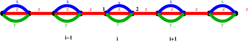
Figure 1: The XYZ-Ising chain. There are two sites per unit cell. The $x,y$ and $z$ bonds are as indicated.

We consider the Hamiltonian,

$$H=\sum_{i=1}^{N}\left(J_{x}\sigma^{x}_{i,1}\sigma^{x}_{i,2}+J_{y}\sigma^{y}_{i,1}\sigma^{y}_{i,2}+J_{z}\sigma^{z}_{i,1}\sigma^{z}_{i,2}+\sigma^{z}_{i,2}\sigma^{z}_{i+1,1}\right)$$ (1)

with periodic boundary conditions,

$$\sigma^{z}_{N+1,1}=\sigma^{z}_{1,1}.$$ (2)

In each unit cell, there is a conserved $Z_{2}$ invariant, $W_{i}=\sigma^{z}_{i,1}\sigma^{z}_{i,2}$. Apart from these $N$ local conserved quantities, there are also three global conserved quantities corresponding to global $\pi$ rotations about each of the three axes which are symmetries of the model. We denote these by, $\Sigma^{a}\equiv\prod_{i=1}^{N}\sigma^{a}_{i,1}\sigma^{a}_{i,2}$ These are not independent, we have $\Sigma^{z}=\prod_{i=1}^{N}W_{i}$ and $\Sigma^{x}\Sigma^{y}=(-1)^{N}\Sigma^{z}$.

Thus, we see that the $J_{z}$ terms in the Hamiltonian (1) are invariants and, hence, do not affect the eigenstates. In this work we concentrate on $J_{x}=J_{y}\equiv\frac{J}{2}$. As we will show, at this point the model is analytically solvable. Also, note that this point the model has a global $U(1)$ symmetry corresponding to spin rotations about the $z$ axis. Leib et al had studied the model at the $J_{z}=J_{x}=J_{y}$ point and had called it the Heisenberg-Ising model. We follow their nomenclature and refer to the model in equation (1) with $J_{x}=J_{y}$ as the $XY$-Ising model.

We express the Hamiltonian in terms of Majorana fermions using the Jordan-Wigner transformation,

$$\xi_{i,1} = (-1)^{i}\sigma^{z}_{i,1}\mu_{i},~{}~{}\xi_{i,2}=(-1)^{i}\sigma^{x}_{i,2}\sigma^{y}_{i,1}\mu_{i}$$ (3)

$$\eta_{i,1} = \sigma^{x}_{i,1}\mu_{i},~{}~{}\eta_{i,2}=\sigma^{z}_{i,2}\sigma^{y}_{i,1}\mu_{i}$$ (4)

where $\mu_{i}=\prod_{i<j}\sigma^{y}_{j,1}\sigma^{y}_{j,2}$.

Then, the Hamiltonian reduces to,

$$H = \sum^{N-1}_{i=1}\left(i\xi_{i,2}\xi_{i+1,1}\right)+\Sigma^{x}~{}i\xi_{N,2}\xi_{1,1}$$ (5)

$$+\sum_{i=1}^{N}\left(J\left(\frac{1-u_{i}}{2}\right)i\xi_{i,1}\xi_{i,2}+J_{z}u_{i}\right)$$

where $\hat{u}_{i}=-i\eta_{i,1}\eta_{i,2}$ and $\prod_{i}^{n}\left(i\xi_{i,1}\xi_{i,2}\right)\prod_{i}^{N}\hat{u_{i}}=\Sigma^{x}$ are conserved quantities.

The Majorana operators $\xi_{i}$ and $\eta_{i}$ follow the anti-commutation relations,

$$\{\xi_{i},\xi_{j}\}=2\delta_{i,j};\{\eta_{i},\eta_{j}\}=2\delta_{i,j};\{\xi_{i},\eta_{j}\}=0.$$ (6)

Thus, the spin Hamiltonian gets converted into the fermionic Hamiltonian with periodic boundary condition when $\Sigma^{x}=+1$ and with anti-periodic boundary conditions when $\Sigma^{x}=-1$.

III Diagonalisation

The Hamiltonian can be diagonalised in the standard way. We write the eigenstates as direct products of states $|{\cal G}\rangle$ in the $\eta$ fermion sector and states $|{\cal M}\rangle$ in the $\xi$ fermion sector. We will refer to states belonging to $\eta$ fermion sector as the gauge sector and states belonging to $\xi$ fermion sector as matter sector. We choose the states in the gauge sector to be the simultaneous eigenstates of the $Z_{2}$ flux operators, i.e $|{\cal G}\rangle=|\{u_{i}\}\rangle$, where

$$\hat{u_{i}}|\{u_{i}\}\rangle=u_{i}|\{u_{i}\}\rangle.$$ (7)

We then have

$$H\left[\hat{u_{i}}\right]|{\cal M}\rangle|\{u_{i}\}\rangle=H\left[u_{i}\right]|{\cal M}\rangle|\{u_{i}\}\rangle.$$ (8)

The single particle eigenvalue equation is given by,

$$\frac{-i}{2}\phi_{i-1,2}+\frac{iJ(1-u_{i})}{2}\phi_{i,2}=\epsilon\phi_{i,1}$$

$$\frac{-iJ(1-u_{i})}{2}\phi_{i,1}+\frac{i}{2}\phi_{i+1,1}=\epsilon\phi_{i,2},$$ (9)

with boundary condition

$$\phi_{1,1}=\phi_{N+1,1}.$$ (10)

We define the $u_{i}=-1~{}\forall~{}i$ sector as the then defect free sector. This zero defect sector consists of two sectors corresponding to periodic or anti-periodic boundary conditions for $\Sigma_{x}=+1$ and $\Sigma_{x}=-1$ respectively. We will prove that this is the ground state sector of the model. If $n$ of the $u_{i}$’s are equal to $+1$ then we call it the $n$-defect sector. An $n$ defect sector reduces to solving the hopping problem on $n$ decoupled open chains. If we can solve one defect sector (one open chain), then we can solve all the sectors of the model because all of them reduce to decoupled open chain Hamiltonians.

IV Exact Solution in all Sectors

In this section we put $J_{z}=0$ since the eigenstates are independent of $J_{z}$. We first consider the zero-defect sector of a chain with $N$ unit cells, in the thermodynamic limit $N\rightarrow\infty$. The Hamitonian is diagonalised in terms of the Fourier components of the Majorana fermion operators,

$$\xi_{i}=\frac{1}{\sqrt{N}}\sum_{k}\xi_{k}e^{-ikR_{i}}$$ (11)

where $R_{i}=ai$, $a$ being the lattice spacing, we have supressed the sub-lattice index and $\xi_{i}$ represent two component column vectors. The hermiticity of $\xi_{i}$ implies that $\xi_{-k}=\xi^{\dagger}_{k}$, their components satisfy the canonical anti-commutation relations,

$$\left\{\xi_{k,a},\xi^{\dagger}_{k^{\prime},a^{\prime}}\right\}=\delta_{aa^{\prime}}\delta{kk^{\prime}}$$ (12)

Fermionic modes are thus defined on half the Brillouin zone. The momentum space Hamiltonian is,

$$H = \frac{1}{\pi}\int_{0}^{\pi/a}~{}dk~{}\xi^{\dagger}_{k}h(k)\xi_{k}$$ (13)

$$\mbox{where}h(k) = \left(\begin{array}[]{cc}0&J-e^{ika}\\ J-e^{-ika}&0\end{array}\right).$$ (16)

The Hamiltonian in the diagonalised form is expressed as

$$H=\frac{1}{\pi}\int_{0}^{\pi/a}~{}dk~{}\epsilon(k)\left((\chi^{+}_{k})^{\dagger}{\chi}^{+}_{k}-(\chi^{-}_{k})^{\dagger}\chi^{-}_{k}\right)$$ (17)

where,

$$\chi_{k}^{\pm} = \frac{1}{\sqrt{2}}\left(\begin{array}[]{c}1\\ \pm e^{-i\alpha_{k}}\end{array}\right)$$ (20)

$$\tan\alpha_{k} = \frac{-\sin(ka)}{J-\cos(ka)}$$ (21)

$$\mbox{and~{}}\epsilon(k) = \sqrt{J^{2}-2J\cos(ka)+1}.$$ (22)

Thus, the sytem is gapped for $J\neq 1$. The values of $k$ are determined by applying the boundary condition (10),

$$ka=\frac{(2m-p)\pi}{N},$$ (23)

where $m=1,2,3\dots N$ and $p=0,1$ for (PBC) and anti-(PBC) respectively.

We now consider the one defect sector. The fermionic system is then an open chain with $N$ unit cells satisfying the boundary conditions,

$$\phi_{0,1}=0$$

$$\mbox{and~{}~{}}\phi_{N,2}=0.$$ (24)

We use the standing waves to diagonalise this open chain single particle Hamiltonian,

$$\phi_{i,a}=\frac{1}{\sqrt{2N}}\sum_{k}\phi_{k,a}e^{ikR_{i}}+\phi_{-k,a}e^{-ikR_{i}}.$$

The boundary conditions (IV) imply that

$$e^{i\alpha_{k}}=e^{i(N+1)ka}.$$ (25)

Thus, $k$ are determined by the solution of,

$$ka=\frac{n\pi}{N+1}+\frac{\alpha_{k}}{N+1}.$$ (26)

We have solved equation (26) numerically for $N=10$ and plotted $k$ versus $n$ for $J>1$ and $J<1$ as shown in figure 2.

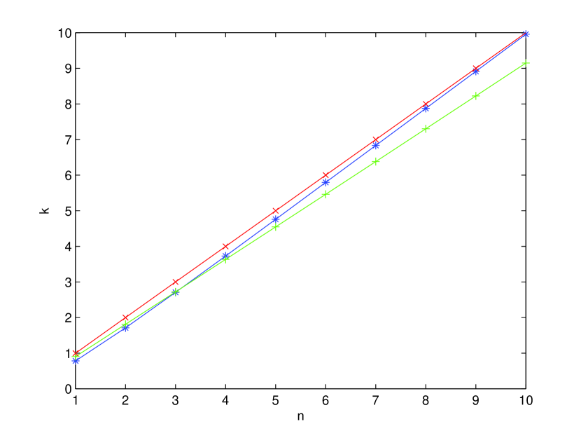
Figure 2: The red line shows the plot between $k$ and $n$ without the correction $\alpha_{k}$. The green and blue line shows the plot between $k$ and $n$ for $J<1$ and for $J>1$ respectively.

We see the number of allowed values of $k$ is $N$ for $J>1$ but is $N-1$ when $J<1$. As we will show later, the missing mode is a zero energy eigenfunction of the single particle Hamiltonian with the wavefunction peaked at the edges of the open chain. The relation $J-e^{ika}=\epsilon_{k}e^{i\alpha_{k}}$ has been shown in the Argand plane in the figure (3) and figure (4). The appearance of the zero mode depends on the topology of parameters of Hamiltonian as shown in figure (3) and (4). Zero mode appears when the unit circle shown there encloses the origin. This argument can be generalised to show that if the path circles the origin $\nu$ times, then there will be $\nu$ only $N-\nu$ standing waves. $\nu$ can be identified with a topological invariant of the closed chain in terms of the Berry potential defined on the half-Brillioun zone of the closed chain,

$$A(k)=i\left(\phi_{k}^{\dagger}\partial_{k}\phi_{k}-h.c\right)$$ (27)

where $\phi_{k}$ are the two-component single particle wavefunctions. The topological invariant is the winding number of the relative phase of the two components of the wavefunction along the half Brillioun zone,

$$\nu=\frac{1}{\pi}\int_{0}^{\pi/a}~{}dk~{}A(k)$$ (28)

Figure 3: $J-e^{ika}=\epsilon_{k}e^{i\alpha_{k}}$ in Argand plane. For $J>1$, $\alpha(0)=0$ and $~{}\alpha(\pi)=0$.

Figure 4: $J-e^{ika}=\epsilon_{k}e^{i\alpha_{k}}$ in Argand plane. For $J<1$, $\alpha(0)=0$ and $~{}\alpha(\pi)=\pi.$

The geometric interpretation of $\nu$ is as follows. Consider a general Hamiltonian of the form

$$h(k) = \epsilon(k)\hat{n}(k)$$

$$\mbox{and~{}}\hat{n}(k) = \cos\theta_{k}\tau^{z}+\sin\theta\left(\cos\Omega_{k}\tau^{x}+\sin\Omega_{k}\tau^{y}\right)$$ (29)

where $\tau^{a}$ are the Pauli matrices. The Hamiltonian in equation (16) is the case of $\theta_{k}=\pi/2$ and $\Omega_{k}=\alpha_{k}$. For fully connected near neighbour chains, the off-diagonal terms in the single particle Hamiltonian in equation do not vanish implying that $\theta_{k}\neq 0,\pi$ for any $k$. Further, if $\epsilon_{k}\neq 0$ the Hamitonian in equation (29) represents a mapping of the half-Brillioun zone to the sphere with two points removed (the north and south poles in our convention), which is topologically equivalent to an annulus. Thus, $\nu$ which is the winding number of the map is a topological invariant for the class of gapped chains for which no nearest neighbour hopping amplitude vanishes.

Thus, we expect the zero energy edge state to be robust and independent of disorder in the couplings, provided the system remains gapped and fully connected by nearest neighbour couplings. We will demonstrate this explicitly in a later section.

The solution of the open chain presented above can be used to to solve $n$ defect sector, for any $n$ as these sectors consist of $n$ decoupled open chains.

V Ground state and Gap

In this section, we will prove that zero defect sector is the ground state sector for $J_{z}=0$. In order to prove the statement we first prove that the ground state energy of zero defect sector is less than that of one defect sector for large $N$. We then prove that ground state energy of one defect sector is less than or equal to that of the $n$-defect sector. We then turn on $J_{z}$ and compute regime of the stability of the system to defect formation. We finally compare our results with those of Lieb et. al.Lieb and point out precisely how our proof extends the regime of validity of their result.

First step: We outline the proof that the ground state energy of zero defect sector $GSE_{zds}$ is less that of the one defect sector, $GSE_{ods}$. The details are given in Appendix A. The ground state energies of the two sectors are,

$$GSE_{zds} = -\sum_{k=1}^{N}\epsilon\left(\frac{2k\pi}{N}\right)$$ (30)

$$GSE_{ods} = -\sum_{k=1}^{N}\epsilon\left(\frac{k\pi}{N+1}+\frac{\alpha(k\pi/N+1)}{N+1}\right)$$ (31)

In the thermodynamic limit of $N\rightarrow\infty$, we convert the summations into integrals using the Euler-Maclaurin formula to get,

$$GSE_{zds} = -\frac{N}{\pi}\int_{0}^{\pi}\epsilon(k)dk$$ (32)

$$GSE_{ods} = -\frac{N}{\pi}\int_{0}^{\pi}\epsilon(k)dk+J(1-\delta(J))$$

$$\delta(J) = \frac{1}{\pi}\int_{0}^{\pi}dk\frac{\cos(k)-J}{\sqrt{J^{2}-2J\cos(k)+1}}$$ (33)

We then show in Appendix that $\delta(J)<1$ for all finite $J$, thus proving that the ground state energy of zero defect sector is less than that of the one defect sector.

Second step: Now, we show that the ground state energy of one defect sector is less than that of two defect sector and so on. To show this, we split up Hamiltonian into three parts,

$$H_{L_{1}+L_{2}}=H_{L_{1}}+H_{L_{2}}+H_{12}$$ (34)

where H is the Hamiltonian for one defect sector, $H_{L_{1}}$ and $H_{L_{2}}$ are Hamiltonians of lengths $L_{1},L_{2}$. $H_{12}$ is the link bond between $H_{L_{1}}$ and $H_{L_{2}}$.

From variational principle,

$$\epsilon_{G}\left(L_{1}+L_{2}\right)\leq\langle\psi|H_{L_{1}}+H_{L_{2}}+H_{12}|\psi\rangle$$ (35)

where $\epsilon_{G}\left(L_{1}+L_{2}\right)$ is the ground state energy of Hamiltonian for one defect sector.

Using the trial wave function $|\psi\rangle=|\psi_{L_{1}}\rangle|\psi_{L_{2}}\rangle$, we get

$$\epsilon_{G}\left(L_{1}+L_{2}\right) \leq \epsilon_{G}\left(L_{1}\right)+\epsilon_{G}\left(L_{2}\right)$$ (36)

$$+ \langle\psi_{L_{1}}|\langle\psi_{L_{2}}|H_{12}|\psi_{L_{1}}\rangle|\psi_{L_{2}}\rangle$$

Let us consider the link Hamiltonian $H_{12}=i\xi_{n}\xi_{n+1}$ where $\xi_{n}$ belongs to the Hamiltonian $H_{L_{1}}$ and $\xi_{n+1}$ belongs to the Hamiltonian $H_{L_{2}}$. Then,

$$\langle\psi_{L_{1}}|\langle\psi_{L_{2}}|H_{12}|\psi_{L_{1}}\rangle|\psi_{L_{2}}\rangle=i\langle\psi_{L_{1}}|\xi_{n}|\psi_{L_{1}}\rangle\langle\psi_{L_{2}}|\xi_{n+1}|\psi_{L_{2}}\rangle.$$

Since the expectation value of single $\xi_{n}$ operator in the ground state is zero. Therefore,

$$\epsilon_{G}\left(L_{1}+L_{2}\right)\leq\epsilon_{G}\left(L_{1}\right)+\epsilon_{G}\left(L_{2}\right)$$ (37)

Thus, we have proved that the ground state energy of one defect sector is less than the ground state energy of two defect sector. Similarly, we can prove for two defect sector and so on. Therefore, zero defect sector is the ground state sector at $J_{z}=0$.

We now turn on $J_{z}$ and examine the region of stability of the zero defect sector under defect production. The difference of the ground state energies of the zero and one defect sector for non-zero $J_{z}$ is

$$GSE_{zds}-GSE_{ods}=J(1-\delta(J))+2J_{z}$$ (38)

Thus, the system will become unstable towards defect production when

$$J_{z}<-\frac{J}{2}\left(1-\delta(J)\right).$$ (39)

This extends the result of Lieb et. al. since their proof is not valid for negative values of $J_{z}$.

V.1 Nature of low energy excitations

For $J_{z}>-\frac{J}{2}(1-\delta(J))$, the zero defect is the ground state sector. The first excited state can be either the first excitation in the zero defect sector or the ground state of the one defect sector. The excitation gap in the zero defect sector follows from the single particle spectrum and is given by

$$\Delta=|(1-J)|.$$ (40)

Therefore, model is gapless for $J=1$. Numerically, we have shown that for $J_{z}=0$ first excited state of the model in the region $0<J\leq 0.75$ and $J\geq 1.17$ is the ground state of the one defect sector . The excited state of the zero defect sector is the first excited state in the region $0.74\leq J\leq 1.17$. These results have been shown in figure (5). We also see that the model has a finite gap for all non-zero values of $J\neq 1,0$.

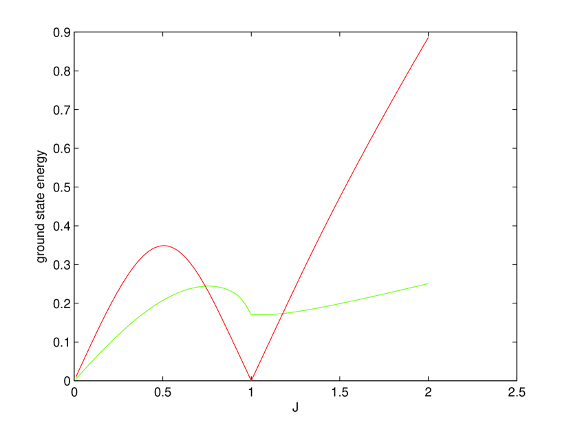
Figure 5: Low energy excitation in XY-Ising Model. The ground state energy of one defect sector is shown in green and first excitation of zero defect sector is shown in red. While plotting all the energies, ground state of zero defect sector has been taken as reference.

VI Zero modes

We now analyse the zero mode of the Majorana fermions. When $\epsilon=0$, equations (III) decouple and become

$$-\frac{J(1-u_{i})}{2}\phi_{i,1}+\phi_{i+1,1} = 0$$

$$\mbox{and~{}~{}}-\phi_{i-1,2}+\frac{J(1-u_{i})}{2}\phi_{i,2} = 0.$$ (41)

These recursion relations can formally be solved,

$$\phi_{i,1} = \prod_{j=1}^{i}\left(\frac{J(1-u_{j})}{2}\right)\phi_{1,1}$$

$$\mbox{and~{}~{}}\phi_{i,2} = \prod_{j=i}^{N}\left(\frac{2}{J(1-u_{j})}\right)\phi_{N,2}.$$ (42)

There are two degenerate and independent solutions for every set of values of the parameters and every flux configuration. In zero defect sector, imposing boundary condition $\phi_{1,1}=\phi_{N+1,1}$, we find that the zero modes exist for zero defect sector only at the gapless point $J=1$. In one defect sector, which is an open chain with boundary condition $\phi_{0,1}=\phi_{N,2}=0$, $\phi_{i,1}$ and $\phi_{i,2}$ can be expressed as,

$$\phi_{i,1} = {\left(J\right)}^{i}\phi_{0,1}$$

$$\mbox{and~{}~{}}\phi_{i,2} = {\left(\frac{1}{J}\right)}^{i-1}\phi_{N,2}.$$ (43)

We can see that if $J>1$, then $\phi_{i,2}$ becomes zero at the boundary for infinite open chain. Now, if we take $\phi_{i,1}=0\forall i$, then the boundary condition at the other end $\phi_{0,1}=0$ is also satisfied for $u_{1}=-1$. Therefore, the only one solution for zero mode exist in an infinite chain for $J>1$. The same is true for the case $J<1$. In both cases, we get only one non-zero solution for zero mode.

Thus, the zero mode occurs when the toplogical invariant is non-zero. It can also be seen from the recursive solution presented above that the zero modes exist even if the coupling, $J$ varies with $i$. Thus the zero mode topologically protected against random, spatial variations in the exchange coupling.

VII Conclusion

To summarize, we have analysed an exactly solvable spin-1/2 chain which was earlier studied by Lieb, Shultz and Mattis Lieb . We have shown that it is a generalised Kitaev chain. Using the methods of Kitaev kitaevhc we can reproduce the earlier results. The formalism also helps us extend the earlier proof to negative vlaues of $J_{z}$ and compute the value of $J_{z}$ when the defect free state becomes unstable to defect production. In addition we have explicitly displayed the topological nature of the zero energy modes in the presence of defects. We have identified the topological invariant that determines the existence of zero energy edge modes in the system. Thus the degeneracy is protected against random variations in the exchange coupling.

In conclusion, our results show that zero energy Majorana modes can be created and manipulated in this model exactly in the same way shown in previous workabhinav . The system has a gap for all non-zero values of $J\neq 1$. Thus the UMF can used as a topological qubit. The importance of this model is that it has only two-spin couplings which can, in principle, be realised experimentallynori .

Appendix A Details of proof

The ground state energy $GSE_{zds}$ of zero defect sector is expressed as

$$GSE_{zds}=-\sum_{k=1}^{N}\epsilon\left(\frac{2k\pi}{N}\right),$$ (44)

where $\epsilon(k)=\sqrt{J^{2}-2J\cos(ka)+1}$.

To evaluate the summation series we convert it into integral using Euler-Maclaurin formula,

$$\sum_{x=1}^{n}f(x) = \int_{0}^{n}f(x)dx+B_{1}[f(0)-f(n)]$$ (45)

$$+ \sum_{k=1}^{p}\frac{B_{2k}}{(2k)!}\left(f^{(2k-1)}(n)-f^{(2k-1)}(0)\right)$$

where $B_{1}=-1/2,B_{2}=1/6,B_{3}=0,B_{4}=-1/30,B_{5}=0,B_{6}=1/42...$ are the Bernoulli numbers.

The expression for ground state energy for zero defect sector equation (44) in thermodynamic limit $N\rightarrow\infty$ becomes,

$$GSE_{zds}=-\frac{N}{\pi}\int_{0}^{\pi}\epsilon(y)dy.$$ (46)

where we have used the identity $\epsilon(0)=\epsilon(2\pi)=J+J_{z}$.

The ground state energy $GSE_{ods}$ of one defect sector is,

$$GSE_{ods}=-\sum_{k=1}^{N}\epsilon\left(\frac{k\pi}{N+1}+\frac{\alpha(k\pi/N+1)}{N+1}\right)$$ (47)

To evaluate the summation series, we convert it into integral using Euler-Maclaurin formula and neglect last terms containing (N+1) in the denominator in limit $N\rightarrow\infty$,

$$GSE_{ods} = -\int_{0}^{N}\epsilon\left(\frac{k\pi}{N+1}+\frac{\alpha(\frac{k\pi}{N+1})}{N+1}\right)dk$$ (48)

$$+ \frac{1}{2}\epsilon\left(\frac{\alpha(0)}{N+1}\right)$$

$$- \frac{1}{2}\left[\epsilon\left(\frac{N\pi}{N+1}+\frac{\alpha(\frac{N\pi}{N+1})}{N+1}\right)\right].$$

In the thermodynamic limit $N\rightarrow\infty$, above equation (48) becomes,

$$GSE_{ods} = -\int_{0}^{N}\epsilon\left(\frac{k\pi}{N+1}+\frac{\alpha(k\pi/N+1)}{N+1}\right)dk$$ (49)

$$+ \frac{1}{2}\left[\epsilon(0)-\epsilon(\pi)\right].$$

Let us substitute $y=\frac{k\pi}{N+1}$, and above expression for ground state energy for one defect sector becomes

$$GSE_{ods} = -\frac{N+1}{\pi}\int_{0}^{\frac{N\pi}{N+1}}\epsilon\left(y+\frac{\alpha(y)}{N+1}\right)dy$$ (50)

$$+ \frac{1}{2}\left[\epsilon(0)-\epsilon(\pi)\right].$$

Using Taylor expansion and neglecting terms containing $\frac{1}{N+1}$,

$$GSE_{ods} = -\frac{N+1}{\pi}\int_{0}^{\frac{N\pi}{N+1}}\epsilon(y)dy$$ (51)

$$- \frac{1}{\pi}\int_{0}^{\frac{N\pi}{N+1}}\left(\alpha(y)\epsilon^{\prime}(y)\right)dy.$$

Using integration by parts in the second term and then taking the thermodynamic limit, we get

$$GSE_{ods}= - \frac{N}{\pi}\int_{0}^{\pi}\epsilon(y)dy$$ (52)

$$- \frac{1}{\pi}\int_{0}^{\pi}dy\frac{J\cos(y)-J^{2}}{\sqrt{J^{2}-2J\cos(y)+1}}$$

$$+ \frac{1}{2}\left[\epsilon(0)+\epsilon(\pi)\right]$$

$$+ \frac{1}{\pi}\left[\alpha(\pi)\epsilon(\pi)+\alpha(0)\epsilon(0)\right].$$

From figures (3, 4),

$$\epsilon(0) = J+1$$

$$\epsilon(\pi) = J-1~{}~{}when~{}~{}J>1$$

$$\epsilon(\pi) = 1-J~{}~{}when~{}~{}J<1$$

$$\alpha(0) = 0$$

$$\alpha(\pi) = 0~{}~{}when~{}~{}J>1$$

$$\alpha(\pi) = \pi~{}~{}when~{}~{}J<1.$$ (53)

Substituting all these values, we show that for both cases $J>1$ and $J<1$ ground state energy of one defect sector is expressed as,

$$GSE_{ods} = GSE_{zds}+J(1-\delta(J))$$

$$\mbox{where~{}}\delta(J) = \frac{1}{\pi}\int_{0}^{\pi}dy\frac{\cos(y)-J}{\sqrt{J^{2}-2J\cos(y)+1}}.$$ (54)

Since in the expression for $\delta(J)$ the integrand is always less than 1, we can write

$$\delta(J) < \frac{1}{\pi}\int_{0}^{\pi}dy=1.$$ (55)

Therefore, from equation (54), we can say that the ground state energy of zero defect sector is less than ground state energy of one defect sector.

References

- (1) E. Lieb, T. Schultz, and D. Mattis, Annals of Physics: 16, 407-466 (1961).
- (2) C. Nayak, S. H. Simon, A. Stern, M. Freedman, and S. D. Sarma, Rev. Mod. Phys. 80, 1083 (2008).
- (3) A. Kitaev, Usp. Fiz. Nauk (Suppl.) 171, 131 (2001).
- (4) A. Y. Kitaev, Ann. Phys. (N.Y) 303, 2 (2003), A. Y. Kitaev, Ann. Phys. (N.Y) 321, 2 (2006).
- (5) J. Alicea, Yuval Oreg, G. Refael, Felix von Oppen, and M. P. A. Fisher, Nature Physics, 7, 412 (2011).
- (6) Lara Faoro, Jens Siewert, and Rosario Fazio, Phys. Rev. Lett. 90, 028301 (2003).
- (7) H. Yao, and S. A. Kivelson, Phys. Rev. Lett. 99, 247203 (2007).
- (8) S. Yang, D. L. Zhou, and C.P. Sun, Phys. Rev. B 76, 180404(R) (2007).
- (9) S. Mandal, and N. Surendran, Phys. Rev. B 79, 024426 (2009).
- (10) Z. Nussinov, and G. Ortiz, Phys. Rev. B 79, 214440 (2009).
- (11) Baskaran, G. Santhosh, and R.Shankar, arXiv:0908.1614 (2009).
- (12) Uma Divakaran, and Amit Dutta, Phys. Rev. B 79, 224408 (2009).
- (13) L. M. Duan, E. Demler, and M. D. Lukin, Phys. Rev. Lett. 91, 090402 (2003).
- (14) J.Q. You, X. F. Shi, X. Hu, and Franco Nori, Phys. Rev. B 81, 014505 (2010).
- (15) A. Saket, S. R. Hassan, and R. Shankar, Phys. Rev. B 82, 174409 (2010).