Reconstructing the Properties of Dark Energy using Standard Sirens

Abstract

Future space-based gravity wave experiments such as the Big Bang Observatory (BBO), with their excellent projected, one sigma angular resolution, will measure the luminosity distance to a large number of gravity wave (GW) sources to high precision, and the redshift of the single galaxies in the narrow solid angles towards the sources will provide the redshifts of the gravity wave sources. One sigma BBO beams contain the actual source only in 68 per cent cases; the beams that do not contain the source may contain a spurious single galaxy, leading to misidentification. To increase the probability of the source falling within the beam, larger beams have to be considered, decreasing the chances of finding single galaxies in the beams. Saini, Sethi and Sahni (2010) argued, largely analytically, that identifying even a small number of GW source galaxies furnishes a rough distance-redshift relation, which could be used to further resolve sources that have multiple objects in the angular beam. In this work we further develop this idea by introducing a self-calibrating iterative scheme which works in conjunction with Monte-Carlo simulations to determine the luminosity distance to GW sources with progressively greater accuracy. This iterative scheme allows one to determine the equation of state of dark energy to within an accuracy of a few percent for a gravity wave experiment possessing a beam width an order of magnitude larger than BBO (and therefore having a far poorer angular resolution). This is achieved with no prior information about the nature of dark energy from other data sets such as SN Ia, BAO, CMB etc.

A remarkable property of our universe is that it is accelerating. The cause of cosmic acceleration is presently unknown and theorists have speculated that it might be due to the presence of the cosmological constant, an all pervasive scalar field called Quintessence, a Born-Infeld type scalar called the Chaplygin gas, etc. It has also been suggested that modifications to the gravity sector of the theory, such as extra dimensional ‘braneworld’ models or $f(R)$ theories, might be responsible for cosmic acceleration. Establishing the nature and cause of cosmic acceleration is clearly a paramount objective of modern cosmology DE ; DE1 . Standard candles in the form of type Ia supernovae (SNIa) and standard rulers such as baryon acoustic oscillations (BAO) observed in the clustering of galaxies, have played a key role in garnering support for the accelerating universe hypothesis. Standard candles rely on an accurate determination of the luminosity distance to infer the expansion history and to make a case for cosmic acceleration. As pointed out in schutz86 ; decigo ; holz051 ; arun ; sathya a complementary probe of the expansion history is available in the form of gravitational radiation emitted from compact binary objects such as neutron star - neutron star (NS-NS) binaries, neutron star - black hole (NS-BH) binaries, or black hole - black hole (BH-BH) binaries.

Indeed, it appears that if the underlying physics behind gravitational radiation emitted by a NS-NS binary is well understood, then the luminosity distance to a given redshift, $D_{L}$, can be established to a (intrinsic) precision of about 2% hirata2010 , making this binary an excellent standard siren. However, for a single source the dominant uncertainty is due to weak lensing, which is 2-3 times this precision. What is needed additionally, to determine $D_{L}(z)$, is the source redshift of the compact binary emitting gravitational radiation, and the main systematic uncertainty in this case is the possible misidentification of the galaxy hosting the binary object (see e.g. holz051 ; arun ; sathya ).

Figure 1: This figure shows the posterior probability distribution $P(z)$ produced by a linear model for $D_{L}$ using the Chebyshev polynomials (6). The solid line shows the exact expression for $P(z)$ given by (A9) of S3, while the dotted line shows the approximate expression for $P(z)$, given by (A12) of S3, and which is used in this paper – see (10). The two methods of determining $P(z)$ agree very well.

The proposed space-borne gravitational wave observatory LISA lisa was expected to achieve an angular resolution of about $1^{\prime}$, and the volume bounded by this angle is expected to contain roughly $30$ objects at $z\simeq 1$ holz051 . Its replacement eLISA will have a considerably lower angular resolution (several degrees) and will therefore contain far more objects within its field of view elisa . Thus unless the galaxy hosting the binary system can be unambiguously identified by the electromagnetic afterglow of the merger event bense08 , the large number of objects within the eLISA beam will compound the problem of host identification. Even in the complete absence of electromagnetic afterglow from GW sources, it seems possible to obtain useful cosmological information: In a key paper, MacLeod & Hogan macleod showed that by considering all the galaxies inside the error box as equally likely sources of a given GW emission, the Hubble parameter can be measured to an accuracy of better than a per cent. Their argument is based on observations of stellar mass black holes inspiralling into massive black holes, the so-called extreme mass ratio inspiral or EMRI events. These events would be dominant at $z<1$ where the weak lensing uncertainty is small. Since galaxies are strongly clustered, and the sources are equally likely to happen in galaxies irrespective of their clustering, cluster redshifts would dominate the averaging procedure inside the error box, thereby providing statistical information about the host redshift. Our paper builds upon this earlier work macleod and shows how one can iteratively pin down the $D_{L}$-$z$ relationship even in the absence of an electromagnetic afterglow from GW sources.

Clearly, then, the major source of uncertainty in determining $D_{L}(z)$ using standard sirens is caused by the misidentification of the galaxy hosting the standard siren, and the chances for this to happen increase with the number of galaxies within the observational beam. Since gravity wave standard sirens have enormous potential for ascertaining the nature of dark energy, it would clearly be very desirable to minimize this source of systematics. Luckily one expects a substantial improvement in the directional sensitivity of next generation gravitational wave (GW) experiments. Indeed, space observatories such as DECIGO decigo , the Big Bang Observer (BBO) BBO and ASTROD Ni , currently in the planning stage, are likely to have a directional sensitivity of a few arc seconds or better, in which case one might expect only a single galaxy to fall within the field of view for a large fraction of observing directions holz09 . These space based observatories are expected to measure the equation of state of dark energy to an unprecedented accuracy holz09 ; zhao11 . Although BBO/DECIGO experiments are in reality at a conceptual stage, for the purpose of this paper we treat the above mentioned characteristics as a generic stand in for a future highly advanced gravitational-wave mission and use the label BBO/DECIGO as a convenient abbreviation for such a mission.

Interestingly, even in the absence of an electromagnetic signature, the source galaxy of the GW signal can still be singled out from amongst the several galaxies lying within the observational beam if its redshift is consistent with the luminosity distance derived from an approximately known cosmology. Utilizing this idea ((saini10, ), hereafter S3) suggested an iterative scheme to identify the source galaxy of the (unresolved) GW signal. At the start of the iterative scheme, reliably identified GW sources — called ‘gold plated’ (GP) sources, following holz09 —give a first estimate of the relationship between the luminosity distance and redshift (henceforth called the DZ relation ¹ ). The expected number of GP sources depends crucially on the directional sensitivity of the experiment: good directional sensitivity will result in a large number of GP sources whereas the opposite will be true for an experiment with poor sensitivity. The reason for this is simple, an experiment with good sensitivity will frequently have a single galaxy within its beam and optical follow ups could establish its redshift.

However, even if one commences with fewer GP sources at the beginning, one can still improve the DZ relation iteratively as follows. For poor directional sensitivity (large angular uncertainty) most GW signals would be unresolved since several galaxies would fall within the (large) angular beam. However, even in this case, a (rough) DZ relation derived from GPs can single out one particular galaxy – the one which is most consistent with the DZ relation – to be the source. This increases the resolved set, thereby improving the DZ relation, and this procedure can now be used iteratively. As more and more sources are resolved, the estimate for the DZ relation improves and eventually saturates at the point when uncertainty in the redshift of the source is dominated by instrumental and lensing scatter rather than by our empirical knowledge of $D_{L}(z)$.

S3 investigated the efficacy of this method analytically, using the ensemble average of statistical quantities at each step of the iteration. Analytically the iteration scheme yields a recursion relation of the form $N_{j+1}=f(N_{j})$, where $N_{j}$ is the number of resolved sources at the $j$th step of the iteration. The limiting number of resolved sources is then obtained by solving $N=f(N)$, which is reached after an infinite number of essentially infinitesimal improvements. In practice, we expect the iterations to freeze much sooner due to Poisson fluctuations since the number of resolved sources at each step of the iteration is in reality a rapidly decreasing random number, and is therefore not expected to change monotonically.

Figure 2: This plot shows the number of gold plated sources (at the commencement of our iteration) as a function of total number of events. Note the excellent agreement between the theoretical prediction in Eq 16 (dashed line) and the simulation (filled hexagons).

A crucial aspect of this method is the definition of the error box into which we expect the source to fall. The data only informs us that the source of the GW signal falls within a solid angle with a given probability; and the measured noisy luminosity distance to the source, along with the DZ relation, informs us that the source redshift falls within a redshift interval with a given probability. Therefore, given an error box we cannot be certain that the true source of the GW signal lies within it. S3 used one sigma BBO beams with one sigma redshift range (inferred from noise in the measured luminosity distance) to define the error box. However, the assumption of localizing the source galaxy within the one sigma error box is fraught with difficulties: if we assume Gaussian noise then the one sigma error box contains the true source only in 68 per cent of cases, the left-over 32 per cent tail will either contain no galaxy or a non-source galaxy. In the case when the error box is empty there is no problem since it leads to an unresolved source, however, if the error box contains the wrong galaxy, with a redshift different from the true source, the inclusion of this DZ pair into the GP set will bias the DZ relation. The misidentified sources are a problem in general, but more seriously, their specific impact on the iterative process is to drive the inferred cosmology away from its true value because a biased DZ relation would deem non-sources as being closer to the biased DZ relation, causing the number of misidentifications to increase with iterations and thereby increasing the bias. On the other hand, choosing a larger error box to decrease the chances of misidentification increases the number of galaxies falling inside the error box, thereby decreasing the chance of resolving the GW signal. Clearly, the size of the error box needs to be chosen in a manner that ensures that misidentifications remain small but not at the cost of resolving as many sources as possible. A useful recipe is to start with the smallest error box, implying the largest number of misidentified sources, and increasing its size until the bias becomes smaller than the random errors.

On the average, the BBO/DECIGO one sigma angular beam would not contain the true source in 32 per cent cases but may contain a non-source galaxy, leading to misidentification. The only way to ensure that beams do contain the true source galaxy is to consider larger beams and regard all galaxies falling in, for example, $n\Delta\Omega_{\rm BBO}(z)$ beam ($n\sim\rm few)$, to be potential sources. This ensures that there are very few beams which do not contain the true source. However, as mentioned above, this will decrease the total resolved set and therefore should affect the inferred cosmological constraints. Surprisingly, the dark energy equation of state can be reconstructed remarkably well even for $n$ as large as $n=10$, as we demonstrate in this paper.

Our main motivation for the present work is to investigate the above issues in detail through Monte-Carlo simulation of data; and to explore choices for the error box that lead to a well determined DZ relation with minimal bias.

I Self-calibration with Monte-Carlo simulated data

A realistic Monte-Carlo simulation mimicking the outcome of the BBO/DECIGO experiment requires a careful consideration of the astrophysical aspects of the problem. First, we have to assume something about the type of galaxies that would host NS-NS binary systems, and their abundance, to derive the rate of NS-NS merger events as a function of redshift. The number of resolved sources as a function of redshift decides how well the DZ relation is established, which in turn decides the precision with which one can reconstruct the properties of dark energy. A detailed prescription for sources of GW signals is presently not well known and depends on theories of stellar and galactic evolution, and in this work we continue to use the rates used in Eq 2 of holz09 . However, the main issue we are investigating here is the efficacy of identification of the source galaxies for GW signals using the DZ relation. Therefore this prescription is entirely adequate for our purposes. We believe that the achievable precision on cosmology quoted in our paper is likely to be fairly representative.

For localizing the source galaxy, the prime uncertainty is due to the presence of other galaxies in the error box; therefore, it is also necessary to assume something about the spatial distribution of galaxies. If the galaxies are clustered in redshift then identification of the source galaxy becomes relatively more difficult. It is well known that galaxies cluster in a complex manner, with the clustering depending both on galaxy type as well as redshift. Using the two-point correlation function, S3 gave an estimate of the effect of clustering on the number of galaxies that are expected to fall within an error box. Basically, the net effect is to increase the number of galaxies in the vicinity of the actual source galaxy since the source galaxy is more likely to lie in a clustered environment. Although it is desirable to simulate data taking into account the clustering of galaxies, this turns out to be a difficult task. For the purposes of the present paper we shall neglect this effect and use the approximation that galaxies are distributed uniformly randomly at each redshift (our method is described in greater detail below). As our previous analysis of the two-point correlation function indicates saini10 , this will lead to slightly optimistic estimates of the final achievable cosmological constraints.

I.1 Simulating Data

The simulated data described below has for each GW signal an associated: redshift of the source galaxy; redshifts of some (or none) non-source galaxies; the angular beam size at the source redshift; and the noisy distance estimate along with an estimate for the error in the distance. We call this data, collectively associated with a single source, as a pencil. We earlier mentioned that if one considers only one sigma angular resolution then not all BBO beams will contain the source galaxy. In our simulation each pencil, by construction, contains a galaxy at the source redshift. Since a one sigma angular beam on an average contains the source in 68% of the cases, this amounts to assuming the total number of simulated sources to be about 50 per cent higher. Of the 32 per cent beams that do not contain the true source, a small percentage could contain a non-source galaxy which would mistakenly be deemed to be a gold plated source. In our prescription these misidentified sources are not taken into account. As we demonstrate later, even if we choose an angular beam of size $10\Delta\Omega_{\rm BBO}$, our method succeeds in resolving the redshifts of enough GW sources so that the implied constraints on dark energy are only marginally worse than what one obtains for a one sigma beam. Such large angular beams are almost certainly going to contain the source galaxy, therefore this prescription does not lead to any distortion in our conclusions for larger beam sizes. However, the results quoted for smaller angular beams would appear to contain smaller bias than would be the case had we included the misidentified sources.

To populate non-source galaxies in the beams we divide the redshift range into a large number of redshift bins. Following holz09 , we consider sources up to $z=5$. As mentioned earlier, we ignore the clustering of galaxies, therefore, we assume that galaxies are distributed uniformly randomly in each redshift bin $\Delta z_{\rm bin}$. The mean number of galaxies, $\bar{n}$, lying within the beam at a given redshift bin depends on the size of the bin $\Delta z_{\rm bin}$ and the angular size of the beam $\Delta\Omega(z)$, and is given by (holz09, ; kaiser, ; hu, )

$$\bar{n}(z)\simeq\frac{4N_{\Omega}}{h(z)\sqrt{\pi}}r(z)\,\exp\left[-r^{4}(z)\right]\Delta\Omega(z)\Delta z_{\rm bin}\,,$$ (1)

where we have assumed a small $\Delta z_{\rm bin}$, so the linear approximation in this equation suffices. Here $r(z)=\int_{0}^{z}dz/h(z)$ is the $c/H_{0}$ normalized coordinate distance, $h(z)=H(z)/H_{0}$ and $N_{\Omega}=1000\,\,\rm arc\,min^{-2}$ is the projected number density of galaxies consistent with the Hubble Ultra Deep Field hudf . Given $\bar{n}$, the probability that there be $k$ galaxies in the bin is given by

$$\Pr(k)=\bar{n}^{k}\exp(-\bar{n})/k!\,.$$ (2)

Using a Poisson random generator we then populate each redshift bin with non-source galaxies. The one sigma BBO angular resolution, $\Delta\Omega_{\rm BBO}$, ranges from $1$—$100$ arcsec² and for this work we have adopted the redshift dependence of the BBO beam for NS-NS mergers from Fig 4 of holz09 . For the BBO beam most of these bins do not contain any non-source galaxies since $\bar{n}\ll 1$. In principle, the redshift distribution of GW sources can differ from that of galaxies due to the redshift dependent rate of NS-NS mergers, which we have adopted from Eq 2 of holz09 . Note that the NS-NS rate peaks at $z=1$, which is close to where the galaxy density peaks, so these two distributions are similar to each other (also see figure 4).

To complete the specification of data we also need a noisy estimate of the luminosity distance to the GW source. The dimensionless standard deviation $\sigma_{m}(z)/D_{L}$ is partly due to the fact that the luminosity distance to a GW source cannot be measured to better than about $2\%$ relative accuracy (due to random instrumental noise) and partly due to weak lensing. The uncertainty due to template fitting could be, at least, comparable to that due to instrumental error cutler2007 , however, in this work we do not include them in our analysis. The dominant uncertainty is due to lensing. Lensing produces an asymmetric distribution of magnifications: a majority of the GW sources are demagnified but a tiny fraction of them are highly magnified. If the redshifts of the highly magnified sources are resolved independently then it is possible to handle them statistically; if not then such sources would either lead to misidentifications or would not be resolved at all. However, for our purposes we set aside this complication² and assume that the distribution is described by a symmetric Gaussian distribution with a dimensionless standard deviation $\eta_{\rm wl}(z)=0.042z$, that is derived from the results of holz05 . We add to the lensing standard deviation a fixed random instrumental/template noise with the dimensionless standard deviation given by $\eta_{\rm inst}=0.02$, to obtain the standard error in the luminosity distance $\sigma_{m}$ given through

$$\frac{\sigma_{m}}{D_{L}}=\sqrt{\eta_{\rm wl}^{2}+\eta_{\rm inst}^{2}}~{}.$$ (3)

Using a Gaussian random number generator with this standard deviation, we then assign a noisy distance measurement to each galaxy.

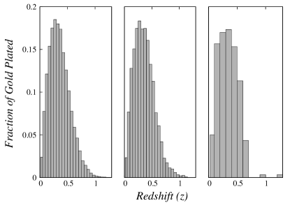
Figure 3: Left panel displays the distribution of gold plated sources with redshift, with total number of GW sources being 300,000, 30,000, 3,000, from left to right. Right panel is a plot of function $\phi(z_{s})$ (Eq. 18). As discussed in the text, these two plots can be combined to obtain the fractional number of GPs for an $n~{}\times$ BBO beam (nBBO) at a given redshift by multiplying the numerical value in the left panel and the numerical value in the right panel raised to power $n-1$.

II Using the DZ relation to increase the number of resolved sources

If a pencil contains only a single galaxy (i.e. non-source galaxies are absent in the beam) then the host galaxy is obviously identified (note that, by construction, all pencils contain the source galaxy), and so it can be used to portray the DZ relation at the redshift of the source (gold plated source). However, as mentioned earlier, the luminosity distance to a GP source has a non-zero random error due to lensing scatter and measurement noise. So using a GP source one can identify the DZ relation at the redshift of the source only to within a finite accuracy.

If the number of GPs is comparable to the total number of GW signals, then we need go no further, but as noted above, this will happen only if beams at all redshifts are very narrow. The BBO one sigma angular resolution is sufficiently narrow for this to be the case. However, since roughly a third of BBO beams will not contain the true source and might also contain a spurious one – thereby biasing the DZ relation – we shall consider beams of larger size³, to ensure that they more certainly contain the source galaxy. For larger beams the number of GPs could be much smaller than the total number of GW signals, in fact, LISA/eLISA beams are so large that they would have no GPs.

At this stage we have a number of GPs that can be used to further resolve the pencils that have more than the single source galaxy within them. To see how this can be done note that the non-source galaxies would typically have redshifts different from that of the source galaxy. For a given pencil, the (noisy) DZ relationship inferred from the GPs provides the probability distribution for the expected source redshift, $P(z)$, for the signal. Clearly, the galaxy in a pencil that is closest to the peak of this distribution is more likely to be the actual source galaxy. The appendix in S3 gives a detailed Bayesian method for determining this probability distribution using a linear fitting function (linear in parameters of the model) for the luminosity distance. According to this method, the GP sources are used to infer the DZ relation by fitting them to a linear model for the DZ relation, namely

$$D_{L}(z,\boldsymbol{\rm h})=\sum_{i}^{N}h_{i}f_{i}(z)=\boldsymbol{\rm h}^{\rm T}\boldsymbol{\rm f}\,,$$ (4)

where $\boldsymbol{\rm h}$ are the $N$ parameters of the model, $f_{i}$ are $N$ arbitrary functions of redshift, and we have defined $\boldsymbol{\rm f}=\{f_{1}(z),f_{2}(z),\ldots,f_{N}(z)\}$. The number of terms in the fitting function is decided by the quality of data: better quality data requires larger $N$ to adequately fit data. Moreover, the choice of functional form of $f_{i}$ should ensure that the fitting function, for some values of parameters $\boldsymbol{\rm h}$, is able to mimic the behavior of the target DZ relation.

After constructing an appropriate fitting function, the model is fitted to the resolved sources and the errors on the parameters of the fitting function are obtained. They are described by the Gaussian distribution

$$P(\boldsymbol{\rm h})=\frac{1}{(2\pi)^{N/2}\sqrt{\det{\boldsymbol{\rm C}}}}\exp\left[-\frac{1}{2}(\boldsymbol{\rm h}^{\rm T}-\boldsymbol{\rm h}^{\rm T}_{0}){\boldsymbol{\rm C}}^{-1}(\boldsymbol{\rm h}-{\boldsymbol{\rm h}}_{0})\right]\,,$$ (5)

where ${\boldsymbol{\rm C}}$ is the covariance matrix and $\boldsymbol{\rm h}_{0}$ are the best fit parameters. This fit is then used to infer the posterior probability distribution for the unknown source redshift given the noisy luminosity distance to the GW signal. The resulting expression is straightforward but complicated, and is given by Eq. (A6) of S3.

The Chebyshev polynomials provide a flexible and convenient linear fitting function for the luminosity distance,

$$D_{L}(z,\boldsymbol{\rm h})=\sum_{I=1}^{N}h_{I}{\rm ChebI}(z)\,,$$ (6)

where ${\rm ChebI}(z)$ is the $I$th order Chebyshev polynomial. Depending on the quality of data, the order of fit $N$ can be set at a value where the fit becomes good (in terms of the $\chi^{2}$ test). The reason for choosing Chebyshev polynomials over ordinary polynomials is that the numerical value of these polynomials remains bounded in the range $(-1,1)$, within the range of the fit. This ensures that the statistical errors on the coefficients $h_{i}$ remain similar for all orders $I$. This is extremely important for translating them to errors on redshift through $P(z)$, where the covariance matrix needs to be numerically well behaved for inversion.

We find that this linear model works well most of the time. But in a few high redshift cases the inferred redshift peak fails to fall reasonably close to the true source redshift. This happens because noise in the data affects the fit adversely, especially at high redshifts where the number of resolved sources is small. The polynomial fit is in some sense local and does not respect the expectation of monotonicity, therefore it tries to over-fit any local feature produced by noise; this produces artifacts that need to be handled individually, making it difficult to automate the process.

Due to limitations of a linear Chebyshev polynomial based fit, we considered other alternatives. It is clear that a physics based model for the luminosity distance does not have these limitations. However, a crucial unknown is the physics governing the behavior of dark energy, which is crucial for determining the luminosity distance. The unknown physics of dark energy is usually encapsulated in the form of a fluid model for dark energy, with an equation of state, $p=w\rho$. The unknown function $w$ is then thought of as a function of redshift $w(z)$, and can be parameterized in terms of a suitably versatile fitting function⁴ . For our work we follow the following reconstruction procedure which incorporates the CPL fitting function CPL for $w(z)$ given below:

$$\frac{D_{L}(z)}{1+z}=\frac{c}{H_{0}}\int_{1}^{1+z}\frac{dx}{H(x)}$$ (7)

where,

$$H^{2}(z) = H_{0}^{2}[\Omega_{M}(1+z)^{3}+\Omega_{\rm DE}]^{2}~{},$$

$$\Omega_{\rm DE} = (1-\Omega_{M})\exp{\left\{3\int_{0}^{z}\frac{1+w(z)}{1+z}dz\right\}}~{},$$

$$w(z) = p_{\rm DE}/\rho_{\rm DE}=w_{0}+\frac{w_{1}z}{1+z}~{},$$ (8)

with $\Lambda$CDM corresponding to $w_{0}=-1,\,w_{1}=0$. The CPL ansatz produces reasonable fits if dark energy has a slowly varying equation of state.

However, from the perspective of the iterative scheme which we develop in this paper, this fitting function has a problem: it depends non-linearly on the model parameters $\Omega_{M}$, $w_{0}$ and $w_{1}$. The posterior probability $P(z)$ for the source redshift can be analytically obtained only if the luminosity distance depends linearly on its parameters (see appendix of S3). A possible remedy is to: (i) use the fitting function (7), (8) to the simulated data to obtain the best fit parameters ($\Omega_{M0},w_{i0}$); (ii) then linearize (7) in $\Omega_{M}$ and $w_{i}$ through a Taylor expansion about the best fit parameters:

$$D_{\rm Linear}(z,\theta_{i})\equiv D_{L}(z;\theta_{i0})+\sum_{i}^{3}(\theta_{i}-\theta_{i0})\frac{\partial D_{L}(z;\theta_{i})}{\partial\theta_{i}}\,$$ (9)

where, for brevity, $\{\theta_{i}\}\equiv\{\Omega_{M},w_{0},w_{1}\}$; the derivatives are evaluated at the best fit parameters $\theta_{i0}$. This function is linear in parameters $\theta_{i}$ and can be used to analytically marginalize over the model parameters to obtain $P(z)$. If the original fit is tight, in the sense that the errors on parameters $\theta_{i}$ are small, then the linearized fitting function $D_{\rm Linear}(z,\theta_{i})$ serves as a close approximation to the original.

It turns out that a further simplification is possible that makes our task much simpler. The posterior probability distribution given in Eq. A9 of S3 is not a simple Gaussian distribution. The distribution has a peak at the redshift that the best fit model predicts for the measured noisy distance to the GW signal but its redshift dependence can be complicated. It is however possible to systematically extract its leading local behavior to obtain the Gaussian distribution

$$P(z)=\frac{1}{\sqrt{2\pi}\sigma_{z}}\exp\left[-\frac{(z-z_{0})^{2}}{2\sigma_{z}^{2}}\right]\,,$$ (10)

where $\sigma_{z}=\sqrt{(\sigma_{m}^{2}+\sigma_{c}^{2})}/D^{\prime}_{L}$; the standard error $\sigma_{m}$ is from Eq. 3, and $\sigma_{c}$ is the cosmology error defined in the last section of the Appendix in S3; $D^{\prime}_{L}=\partial D_{L}(z,\theta_{i0})/\partial z|_{z=z_{0}}$; the parameter $z_{0}$ is the best fit redshift inferred for the GW signal and is computed from the prescription given there, but basically it is the redshift inferred for the noisy distance estimate via the best fit model $D_{L}(z;\theta_{i0})$. Note that due to noise in the measured luminosity distance, $z_{0}$ need not coincide with the true source redshift.

In Fig 1 we plot a comparison of $P(z)$ produced by the local Gaussian approximation (10) and the more exact expression A9 of S3 (both distributions are produced by using a Chebyshev polynomial based fit). We find that the Gaussian approximation agrees very well at all redshifts. In fact, the agreement becomes better with an increase in the number of resolved sources because the error bars on parameters become smaller, and A9 of S3 starts approaching a Gaussian distribution. Therefore, the local Gaussian approximation is adequate for our purposes.

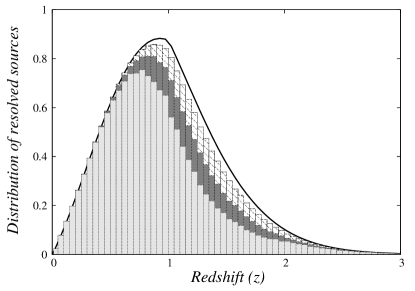
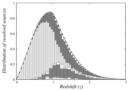
Figure 4: Left panel shows the normalized distribution of resolved GW sources at the end of the iteration. The solid line is the redshift distribution of all sources assuming BBO resolution; dashed lines show the redshift distribution of resolved sources obtained after assuming that the source lies within $1\sigma$ of the peak in the probability distribution $P(z)$ defined in (10). In other words the dashed histogram corresponds to $n=1$ in (11) and $m=1$ in (12). Dark gray shows the same but for a $2\sigma$ allowed region for sources, corresponding to $m=2$ in (12). Finally the light gray shade reflects a $3\sigma$ allowed region for sources and corresponds to $m=3$ in (12). Note that the number of resolved GW sources is comparable to the total number of GW sources for $m=1$ and is only slightly worse for $m=2,3$. Right panel discusses the issue of source misidentification. Clearly by restricting GW sources to lie within an $m\sigma$ region of the peak of the probability distribution $P(z)$ we open up the possibility of source misidentification which is larger for smaller $m$. This is clearly revealed in the inset to the right panel (the shading scheme is the same as in the left panel). We see from this panel that fewer sources are misidentified for $3\sigma$ (light gray) than for $1\sigma$ (dashed). The main panel on the right shows the distribution of resolved sources after misidentified sources have been identified. Thereafter misidentified sources do not play any role in the iterative scheme which, in the case of the dashed region, coincides with the solid line corresponding to the redshift distribution of all GW sources.

II.1 Error Box

The local approximation for $P(z)$ in (10) is convenient in that it enables us to define the error box for the source location in terms of the variance $\sigma_{z}$ of the local approximation Eq 10. Note that this task would be considerably more complicated had we used A9 of S3, which is not described by a few simple parameters as the Gaussian distribution is. To define our error box, let us first choose the beam size in which we expect the source to lie as

$$\Delta\Omega(z)=n\Delta\Omega_{\rm BBO},$$ (11)

where $\Delta\Omega_{\rm BBO}$ is the redshift dependent one sigma resolution of the BBO experiment. The beam has been chosen as a multiple of the BBO resolution to ensure a high probability for the source to fall inside the beam. (This also accommodates the possibility that, as in the case of LISA $\to$ eLISA, the space mission which finally flies has a larger beam width than BBO.) Similarly, we can define the redshift range in which the source is likely to lie as

$$\Delta z=2m\sigma_{z},$$ (12)

which is centered at the peak of the probability distribution $P(z)$. For simplicity, the redshift range has been chosen to be a multiple of the one sigma range obtained from $P(z)$.

II.2 Iterative Scheme

We generate pencils with different values of $n$ in (11). As mentioned above, larger values of $n$ increase the chances of the true source of the gravity wave signal lying within the beam, but have the obvious side effect that the number of non-sources in the beam also goes up. Clearly, with a larger number of non-sources in each beam, the number of gold plated sources (GPs) in the set goes down, therefore, $n$ cannot be chosen too large, otherwise there will be no GPs with which to start our iterative process. The GPs are used to derive an initial estimate of the luminosity distance which is used to infer $P(z)$. Knowing $P(z)$ we repeat the process of going through each pencil and checking whether any (single) galaxy is present in the redshift range $z_{0}-m\sigma_{z}<z<z_{0}+m\sigma_{z}$, where $z_{0}$ corresponds to the peak of $P(z)$. Galaxies inside pencils where this test succeeds are referred to as resolved galaxies and added to the burgeoning inventory of sources. This process is repeated until there is no further increase in the number of resolved sources and the iterative method saturates. Now the final value of the luminosity distance is used to determine $w(z)$ – the equation of state of dark energy, using (7) and (8). Our self-calibrating iterative scheme is summarized below (convergence being reached after $N$ steps):

$${\cal N}^{(1)}_{GP}~{}~{}\longrightarrow~{}~{}D_{L}^{(1)}(z)~{}~{}\longrightarrow~{}~{}P^{(1)}(z)$$

$$P^{(1)}(z)~{}~{}\Longrightarrow~{}~{} {\cal N}^{(2)}_{GP}~{}~{}\longrightarrow~{}~{}D_{L}^{(2)}(z)~{}~{}\longrightarrow~{}~{}P^{(2)}(z)$$

$$\cdots\cdots\cdots\cdots$$

$$P^{(N-1)}(z)~{}~{}\Longrightarrow~{}~{} {\cal N}^{(N)}_{GP}~{}~{}\longrightarrow~{}~{}D_{L}^{(N)}(z)~{}~{}\longrightarrow~{}~{}{\bf w(z)}~{}.$$

Note that as more resolved sources are added, the shape of $P(z)$ becomes peakier and narrower (smaller $\sigma_{z}$), which helps in picking new resolved sources from amongst contender galaxies. This practice, outlined in (LABEL:eq:iterative), is continued until convergence is reached and no new source galaxies can be added to the resolved sample.

Let us illustrate this with an example. Supposing of the 1000 pencil beams that have been generated only 30 have a single galaxy falling within them and the remaining beams contain two or more galaxies. Then we can safely assume that these 30 galaxies host GW sources and, using optical/IR observations, determine their redshifts. This establishes for us our initial DZ relationship, namely $D_{L}^{(1)}(z)$ in (LABEL:eq:iterative), where ${\cal N}^{(1)}_{GP}=30$. Next, knowing $D_{L}^{(1)}(z)$ we determine the probability distribution function, $P^{(1)}(z)\equiv P^{(1)}(z|D_{L}^{(1)})$, through (10). Clearly our knowledge of $P(z)$ will inform us which of the two or more candidate galaxies (in each of the additional 970 beams) is a potential gravity wave source, since this galaxy would lie closer to the peak of $P(z)$ than its companions. Including the resolved galaxy, and others like it, will establish an enlarged sample, and this procedure will be followed iteratively (for $N$ steps) until no new resolved galaxies can be added, at which point we say that convergence has been reached and the final value of $w(z)$ is determined from $D_{L}^{(N)}(z)$ using (7) & (8). If the error box is small (small $n$ and $m$) then it follows that the chances of resolving a GW signal increases since it is more likely that we will find only a single galaxy within the error box. However, a very small error box would also imply that the probability of the true source galaxy lying within it be small, leading to a larger number of misidentifications in this case. Misidentifications have the pernicious effect of biasing the DZ relation away from its true value, resulting in a positive feedback on the chances of misidentifications during later iterations and converting the biasing of the DZ relation into a runaway process. In the other extreme case when the error box is very large, the possibility of misidentification goes down but the chances of resolving GW signals goes down as well, resulting in a decrease in the quality of constraints obtained for cosmology. Clearly then, an optimum value for the error box should be such that the constraints on cosmology are tightest while at the same time the bias is below the statistical scatter.

III Results

At commencement, a small number of gold plated (GP) sources is required in order to obtain the zeroth order cosmology to start our iterative process of statistical resolution of GW sources. The probabilistic expectation value of the number of GP sources for a given number of total sources and the beam size can be estimated as follows: Dividing the redshift range into a large number of bins, the mean number of galaxies $\bar{n}(z_{i})$ in a redshift bin can be estimated through Eq 1 using the angular beam $\Delta\Omega(z_{s})$, where $z_{s}$ is the redshift of the source galaxy; and $\Delta z_{\rm bin}$, where $z_{i}$ is the redshift of the bin.

It is worth noting that the probability for a source to be a GP depends on the angular resolution with which the source can be resolved, therefore the angular resolution of the beam is evaluated at $z_{s}$, thereby making $\bar{n}(z_{i})$ a function of $z_{s}$, which we notate explicitly below. As mentioned earlier, the BBO angular resolution which we have used is taken from Fig 4 of holz09 , corresponding to NS-NS mergers. Our prescription puts the actual source galaxy in each pencil, therefore, the probability that the pencil contains no other galaxy can be obtained from the probability that the redshift bin at $z_{i}$ is empty, which is $\Pr(0)=\exp[-\bar{n}(z_{i};z_{s})]$ (see Eq 2). Clearly, a pencil will give a GP source if all bins are empty⁵ giving a probability

$$\Pr(z_{s};{\rm Gold\,Plated})=\exp\left[-\sum_{z_{i}}\bar{n}(z_{i};z_{s})\right]~{}.$$ (14)

In the expression for $\bar{n}(z_{i};z_{s})$ (Eq 1), we see that it is proportional to the bin size $\Delta z_{\rm bin}$. The probability $\Pr(z_{s};{\rm Gold\,Plated})$, however, is understood to be obtained in the limit of infinitesimal bin size, in which case the sum in the above expression will be replaced with an integration.

For a small enough bin size, defining $f_{s}$ as the fraction of GW sources at redshift $z_{s}$, the fraction of gold plated GW sources at $z_{s}$ is given by

$$f_{\rm GP}(z_{s})=f_{s}(z_{s})\exp\left[-\sum_{z_{i}}\bar{n}(z_{i};z_{s})\right]$$ (15)

and the total number of GPs by

$$N_{\rm GP}=N_{\rm Total}\sum_{z_{s}}f_{s}(z_{s})\exp\left[-\sum_{z_{i}}\bar{n}(z_{i};z_{s})\right]$$ (16)

Fig 2 shows the number of gold plated gravity wave sources as a function of total number of GW sources obtained for the BBO angular beam. As predicted by (16), the theoretical expectation that $N_{\rm GP}\propto N_{\rm Total}$ is found to be true in our simulations. We find that even for a small total number of sources ($\sim 1000$) the GP set is large enough ($\sim 100$). The left panel of Fig 3 plots the function $f_{\rm GP}^{\rm BBO}(z_{s})$. We find that the distribution is independent of the total number of sources, in accordance with theoretical expectation. It is important to note that the distribution of sources in redshift is wide enough for obtaining a good starting DZ $\equiv D_{L}(z)$ relation. Note also that the peak of the redshift distribution $f_{\rm GP}$ of GPs (at $z\sim 0.3$) does not coincide with the peak of the galaxy distribution ($z\sim 1$). This is due to the fact that there is an additional redshift dependence due to the redshift dependent beam size holz09 . The BBO angular resolution is better at smaller redshift; however the number of sources first increase, peak at $z\sim 1$, and then decrease with the redshift; the net effect therefore is to shift the peak of the GPs redshift distribution to a lower redshift.

For larger (than BBO) angular resolution, the number of GPs decreases since the beam, in many cases, becomes too large to accommodate only a single galaxy. This effect can be estimated in terms of the function $f^{\rm nBBO}_{\rm GP}(z)$ for $\Delta\Omega(z)=n\Delta\Omega_{\rm BBO}(z)$, which can be easily shown to be given by

$$f^{\rm nBBO}_{\rm GP}(z_{s}) = f_{s}(z_{s})\exp\left[-n\sum_{z_{i}}\bar{n}_{\rm BBO}(z_{i};z_{s})\right]$$ (17)

$$= f_{\rm GP}^{\rm BBO}(z_{s})\phi^{n-1}(z_{s})$$

$$\phi(z_{s}) \equiv \exp\left[-\sum_{z_{i}}\bar{n}_{\rm BBO}(z_{i};z_{s})\right]\,.$$ (18)

We find that at each redshift, the number of GPs predicted for the $n\Delta\Omega_{\rm BBO}(z)$ beam is smaller than that for $\Delta\Omega_{\rm BBO}(z)$ beam by a redshift dependent multiplicative factor $\phi^{n-1}(z_{s})$. The right panel of Fig 3 plots the function $\phi(z)$. We see that for $z>0.1$, $\phi<1$ is a small fraction; therefore this factor decreases very rapidly with $n$. The multiplicative factor increases with $n$ for $z<0.1$ but since the fraction of sources is small at small redshift, this does not cause an abnormal increase in GPs at low redshift with increasing $n$. Although mathematically speaking this factor blows for large values of $n$, at a large enough $n$ the Poisson statistic will cease to hold, making this argument invalid.

We simulated $300,000$ pencils corresponding to three years of cumulative BBO data. The resolved samples were fitted, at various stages of iteration, with the non-linear model for $D_{L}(z)$ described by (7) in which the CPL equation of state (8) has been used. The model was linearized over the polynomial coefficients and the local approximation discussed earlier was then used to derive $P(z)$. The fiducial model chosen for all our simulations was a flat $\Lambda$CDM model with $\Omega_{m}=0.3$. In all cases (described below) the iterations freeze out after about ten steps implying that convergence had been reached, i.e. $N=10$ in (LABEL:eq:iterative).

In the left panel of Fig 4 we plot the total number of resolved GW sources obtained at the end of our iterative run with $n=1$ in (11) and $m=1,2,3$ in (12). It is interesting that the number of resolved GW sources is comparable to the total number of GW sources for $m=1$ and is only slightly worse for $m=2,3$. The inset in the right panel shows the distribution of misidentified sources (the redshift has been identified incorrectly). Recall that $n=1$ corresponds to the $1\sigma$ angular resolution for BBO and, as pointed our earlier, this implies that roughly a third of all beams will not contain any GW sources at all  ! However, in our simulations we ensure that all pencils do contain the true source, therefore figure 4 does not include the effect of misidentification of sources due to small beam size. The other important cause for misidentifications is due to a choice of too small an allowed redshift range, which is what the inset in figure 4 illustrates (the number of misidentified sources increases as $m$ decreases). The fraction of misidentified sources peaks at $z\sim 1$ because, as mentioned earlier, the BBO beam monotonically becomes wider at larger redshift and so has a larger number of non-source galaxies falling into it; therefore the expected peak redshift for misidentifications is expected to be larger than the peak redshift of the galaxy distribution (albeit only slightly).

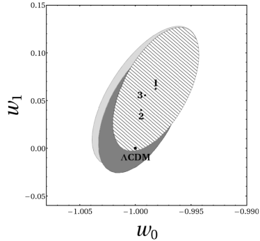
Figure 5: Constraints on $w_{0}$ and $w_{1}$ with misidentified sources included in the resolved sample. The beam size is fixed at the one sigma angular resolution of BBO, corresponding to $n=1$ in (11), while the redshift range in which the source is expected to lie is given by (12), namely $\Delta z=2m\sigma_{z}$. The lined region corresponds to $m=1$, dark gray to $m=2$, and light gray to $m=3$ in (12). In all three cases the fiducial $\Lambda$CDM model ($w_{0}=-1,w_{1}=0$) is included within the one sigma contour, but the fit improves for $m=2,3$, corresponding to a decrease in uncertainty of the source redshift.

In Fig 5 we plot the constraints on $w_{0}$ and $w_{1}$ obtained with $n=1$ and $m=1,2,3$. This figure includes the misidentified sources in order to illustrate how misidentified sources can bias the cosmology. Although the centers of the three one sigma regions (corresponding to three different values of $m$) predict a non-zero variation in dark energy (non-zero $w_{1}$), the fiducial $\Lambda$CDM model ($w_{0}=-1,w_{1}=0$) does fall within the one sigma contour. Also note that larger values of $m$, corresponding to fewer misidentifications, are more consistent with the fiducial $\Lambda$CDM model. Note also that although the 1$\sigma$ contour increases slightly for larger $m$, this effect is pretty marginal.

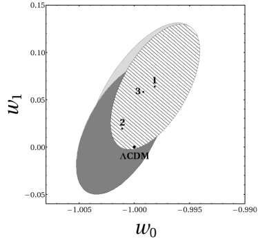
Figure 6: Same as figure 5 but after misidentifications have been removed in the resolved sample. The beam size is fixed at the one sigma angular resolution of BBO, corresponding to $n=1$ in (11). The lined region corresponds to $m=1$, dark gray to $m=2$, and light gray to $m=3$ in (12). In all three cases the fiducial $\Lambda$CDM model ($w_{0}=-1,w_{1}=0$) is included within the one sigma contour. Note that for $m=2$ (dark gray) the fit has improved substantially in comparison with figure 5.

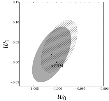
Figure 7: This figure shows the effect of including/excluding misidentified GW sources. The beam size is kept at the BBO one sigma angular resolution corresponding to $n=1$ in (11) and the redshift uncertainty of the source is two sigma: $m=2$ in (12). In this figure the dashed region shows the fit with misidentified sources included and the gray region after misidentified sources have been excluded. As expected, the one sigma contour is in better agreement with the fiducial $\Lambda$CDM model ($w_{0}=-1,w_{1}=0$) if misidentified sources have been excluded from the sample.

This may not be as surprising as it appears. The BBO beam is so narrow that the probability of finding a galaxy within it is small. The one sigma redshift range corresponding to $m=1$ would contain the source galaxy in roughly 68 per cent pencils, while in the remaining cases most pencils would not contain any galaxy at all. Therefore, the total number of misidentifications would be small, and their main role would be in biasing the DZ relation and not so much in controlling the tightness of fit. This is illustrated in Fig 6, which is identical to Fig 5 in all respects other than the fact that here we have removed the misidentified sources. The agreement with the fiducial model is slightly better in this case (especially for $m=2$). The scatter in best fit value is due to the slightly different number of resolved sources in the three cases, however, all three regions are consistent with each other. Fig 7 isolates the effect of including or excluding the misidentified sources. It is clear from this figure that biasing, due to choosing too narrow a redshift range for the source redshift, is present but is smaller than the statistical errors on cosmological parameters.

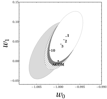
Figure 8: In this figure we illustrate the effect of increasing the beam width on the reconstruction of the equation of state of dark energy. The uncertainty in source redshift remains fixed at $m=1$ in (12) while the beam width increases as $n=1,2,3,10$ in (11), which corresponds to $1\sigma,2\sigma,3\sigma$ and $10\sigma$ times the BBO value. White corresponds to $n=1$, dark gray to $n=2$, dashed to $n=3$ and light gray to $n=10$. Increasing the beam size decreases the overall number of resolved GW sources using which $w(z)$ is reconstructed, and therefore slightly increases the area of the one sigma contour. It is interesting that the fiducial $\Lambda$CDM model ($w_{0}=-1,w_{1}=0$) lies within the $1\sigma$ contour for all values of $n$.

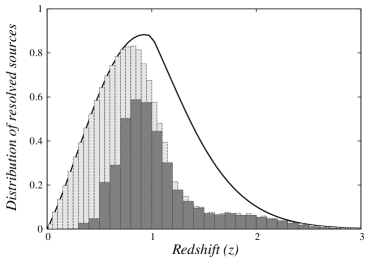
Figure 9: The normalized distribution of resolved sources at the end of our iteration. The solid line is the redshift distribution of all sources. The total fraction of resolved (light gray) and misidentified (dark gray) sources is plotted as a function of redshift for $n=10$ in (11) and $m=1$ in (12).

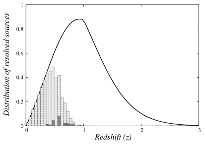
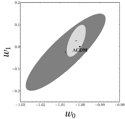
Figure 10: Left panel displays the distribution of resolved sources (light grey) and misidentified sources (dark grey) for $n=10$ in (11) and $m=3$ in (12). (Note the lack of resolved sources beyond $z=1$.) The right panel shows confidence contours for the EOS of dark energy with $n=10$ and $m=1$ (light grey) and $m=3$ (dark grey), respectively.

In Fig 8 we plot the constraints obtained by choosing different beams sizes but keeping the redshift error box at one sigma corresponding to $m=1$ in (12). The beam size chosen for different one sigma regions is $n=1,2,3,10$ in (11), and we find that the area under the one sigma confidence level increases with $n$. This is due to the fact that the total number of GPs decreases with increasing beam size. For this figure the misidentified sources were included in the determination of cosmological parameters. We find that even for $n=10$, which is large enough to ensure that the true source would almost certainly fall within the beam, the constraints are sufficiently narrow, with very little bias, even though as Fig 9 illustrates, the total number of resolved sources in this case is smaller than what one finds for $n=1,2,3$ (compare with figure 4); and the number of misidentifications is large, due to the fact that we have chosen $m=1$ in (12).

The left panel of Fig 10 plots the distribution of resolved sources for $n=10$ and $m=3$, corresponding to the largest error box that we have considered. The number of resolved sources has decreased substantially, however, on the positive side, the number of misidentifications is much smaller than in Fig 9. Note also that there are almost no resolved sources beyond $z=1$. The reason for this is the large source-redshift error at high redshift, which, when taken together with the fact that we are allowing the source to fall in the three sigma redshift range, makes it very difficult to resolve sources. The right panel of the same figure shows the constraints obtained on cosmology. As expected, the constraints are poorer due to lack of sources beyond $z=1$.

The main reason for choosing large $n$ is to ensure that the each beam contains the true source at a greater probability. Our results show that for $n=10$ and $m=1$ the number of resolved sources is sufficient to give good constraints on cosmology, however, the number of misidentifications is large. The bias thus produced is not large and it would seem that this configuration may give us good unbiased constraints on cosmology. However, since our fiducial model has only two parameters, it is possible that the bias may make determining cosmology more difficult for more complicated dark energy models. Therefore, it is necessary to keep the misidentifications small. It is difficult to make general statements regarding the optimum configuration for $n$ and $m$ for a more complicated dark energy model, however, our results suggest that the range $3\leq n\leq 6$ and $2\leq m\leq 3$ may work in most cases.

IV Conclusions

To conclude, we would like to underscore the important point that our self-calibrating scheme works very well even if none of the gravity wave sources have observable electromagnetic signatures. Indeed if the beam width is not too large ($\leq$ ten times BBO), then the presence of only a few gold plated sources (those whose redshift has been independently established) in conjunction with the iterative procedure presented here, allows us to determine the equation of state of dark energy to an accuracy of a few percent – see figure 8. The two main issues investigated in this work are the application of ideas presented in S3 to simulated data, and to address the issue of misidentification of GW sources. Our simulations simplify details in two respects: first, we do not include the effect of clustering, second, we model the lensing scatter as a symmetric Gaussian distribution. (We shall assess the effects of asymmetry induced my lensing as well as the effects of clustering in a companion paper.) We find that the method works quite well on simulated data and the iterations saturate after a small number of steps.

We showed that misidentified sources might in general bias the determination of DZ relation and would lead to a runaway process by which the DZ relation would move away systematically from the true cosmological DZ relation, thus biasing the estimation of the cosmological parameters. In our simulations, the effect of biasing is present but is found to be small. We have shown that increasing the allowed redshift range for the GW source reduces this bias even further, without significantly affecting the cosmological constraints (due to a reduction in the number of resolved sources). A further positive conclusion is that the method works even for larger beam sizes, thereby addressing the concern that not all beams might contain the source galaxy.

In our simulations the asymmetric lensing scatter has been modeled as a symmetric Gaussian distribution. Lensing scatter has a large number of demagnified sources and a small number of compensating large magnifications. As mentioned in holz09 , highly magnified sources would show up as outliers in the DZ plot and can be either removed from the sample or else, in the method that we propose, can be handled by choosing a small value of $m$. As our results show, the bias due to misidentifications is relatively small, so this choice would not cause significant distortions in the estimates of cosmological parameters.

V Acknowledgment

Tarun D. Saini is thankful to the Associateship Programme of IUCAA for providing support for his stay at IUCAA where part of this work was done.

References

- (1) V. Sahni and A. A. Starobinsky, Int. J. Mod. Phys. D 9, 373 (2000); P. J E. Peebles and B. Ratra, Rev. Mod. Phys. 75, 559 (2003); T. Padmanabhan, Phys. Rep. 380, 235 (2003); V. Sahni, Lect. Notes Phys. 653, 141 (2004); V. Sahni, astro-ph/0502032; E. J. Copeland, M. Sami and S. Tsujikawa, Int. J. Mod. Phys. D 15, 1753 (2006); J. A. Frieman, M. S. Turner and D. Huterer, Ann. Rev. Astron. Astroph. 46, 385 (2008); R. Durrer and R. Maartens, ”Dark Energy: Observational and Theoretical Approaches”, ed. P Ruiz-Lapuente (Cambridge UP, 2010), pp. 48 - 91 [arXiv:0811.4132]; S. Nojiri and S. D. Odintsov, Phys.Rept. 505, 59 (2011) [e-Print: arXiv:1011.0544]; T. Clifton, P. G. Ferreira, A. Padilla and C. Skordis, Phys.Rept. 513 1 (2012) [e-Print: arXiv:1106.2476].
- (2) V. Sahni and A. A. Starobinsky, Int. J. Mod. Phys. D 15, 2105 (2006).
- (3) B. F. Schutz, Nature, 323, 310 (1986)
- (4) N. Seto, S. Kawamura, and T. Nakamura, Phys. Rev. Lett, 87 221103 (2001); S. Kawamura, et al., Journal of Physics: Conference Series 122, 012006 (2008); R. Takahashi and T. Nakamura, Prog. Theor. Phys. 113, 63 (2005).
- (5) D. E. Holz and S. A. Hughes, Astrophys. J. , 629, 15 (2005)
- (6) K. Arun, B. Iyer, B. Sathyaprakash, S, Sinha and C. Van Den Broeck, Phys. Rev . D 76, 104016 (2007); Erratum-ibid.D76:129903,2007
- (7) B.S. Sathyaprakash, B.F. Schutz and C. Van Den Broeck, Class.Quant.Grav. 27, 215006, (2010).
- (8) T. Apostolatos, C. Cutler, G. Sussman and K. Thorne, Phys. Rev. D 49, 6274 (1994)
- (9) P. Amaro-Seoane, et al., Class. Quantum Grav. 29, 124016 (2012).
- (10) E.S. Phinney et al., 2003, Big Bang Oberver Mission Concept Study (NASA); A. Nishizawa, K. Yagi, A. Taruya and T. Tanaka, Phys. Rev. D 85, 044047 (2012); A. Nishizawa, A. Taruya and S. Saito, Phys. Rev. D 83, 084045 (2011); J. Crowder and N.J. Cornish, Phys. Rev. D 72, 083005 (2005).
- (11) Wei-Tou Ni, arXiv:1104.5049.
- (12) C. Cutler;M. Vallisneri, Phys. Rev. D., 76, 104018 (2007)
- (13) C. Cutler, D. E. Holz 2009, arXiv:0906.3752v1 [astro-ph.CO]
- (14) C. M. Hirata; D.E. Holz; C. Cutler, Phys. Rev. D., 81, 124046 (2010)
- (15) Zhao, W., van den Broeck, C., Baskaran, D., & Li, T. G. F., Phys. Rev. D., 83, 023005 (2011)
- (16) B. Kocsis, Z. Haiman, and K. Menou, Astrophys. J. , 684, 870 (2008)
- (17) C.L. MacLeod and C.L. Hogan, Phys. Rev. D., 77, 043512 (2008)
- (18) T.D. Saini, S.K. Sethi, & V. Sahni, Phys. Rev. D., 81, 103009 (2010)
- (19) D.E. Holz, and E.V. Linder, Astrophys. J. , 631, 678 (2005)
- (20) M. Chevallier and D. Polarski, 2001, Int. J. Mod. Phys. D 10, 213 [gr-qc/0009008]; E. V. Linder, 2003, Phys. Rev. Lett. 90, 091301 [astro-ph/0208512].
- (21) N. Kaiser, ApJ, 388, 272, (1992)
- (22) W. Hu, ApJ, 522, L21, (1999)
- (23) S.V.W. Beckwith et al. AJ, 132, 1729, (2006).
- (24) K.S. Miller, Mathematics Magazine, Vol. 54, No. 2, pp. 67-72