Bound states in the continuum driven by AC fields

Abstract

We report the formation of bound states in the continuum driven by AC fields. This system consists of a quantum ring connected to two leads. An AC side-gate voltage controls the interference pattern of the electrons passing through the system. We model the system by two sites in parallel connected to two semi-infinite lattices. The energy of these sites change harmonically with time. We obtain the transmission probability and the local density of states at the ring sites as a function of the parameters that define the system. The transmission probability displays a Fano profile when the energy of the incoming electron matches the driving frequency. Correspondingly, the local density of states presents a narrow peak that approaches a $\delta$ function in the weak coupling limit. We attribute these features to the presence of bound states in the continuum.

I Introduction

At the dawn of quantum mechanics, von Neumann and Wigner constructed a spatially oscillating attractive potential that supported a bound state above the potential barrier.Neumann29 This truly localized (square integrable) solution of the time-independent Schrödinger equation is referred to as a bound state in the continuum (BIC). Much later, Stillinger and Herrick reexamined and extended von Neumann and Wigner ideas.Stillinger75 They analyzed a double excited atom model, where BICs were formed and live forever despite the interaction between electrons. They arrived at the conclusion that BICs may be a physically realizable phenomenon in real atomic and molecular systems. In this context, Friedrich and Wintgen discussed in a system of coupled Coulombic channels and, in particular, a hydrogen atom in a uniform magnetic field.Friedrich85 These authors interpreted the formation of BICs as the result of the interference between resonances of different channels. The discovery of a BIC induced by the interaction between two particles in close proximity to an impurity has been recently reported by Zhang et al.,Zhang12 where the state can be tuned in and out of the continuum continuously.

The advent of nanofabrication techniques has made it possible to devise and fabricate quantum devices whose electronic properties are similar to those of atoms and molecules. When the size of the device is comparable to the de Broglie wavelength, one or more degrees of freedom are quantized and the electron wave function is spatially confined. The similarity to atomic systems paved the way to experimentally validate the existence of BICs in artificial nanostructures. Capasso et al. measured the absorption spectrum at low temperature of a GaInAs quantum well with Bragg reflector barriers produced by a AlInAs/GaInAs superlattice.Capasso92 A well defined line at $360\,$meV in the spectrum was attributed to electron excitations from the ground state of the quantum well to a localized level well above the AlInAs band edge. Nevertheless, this state cannot be regarded as a true BIC but a bound state above the barrier since it is a defect mode residing in the minigap of the superlattice, as pointed out by Plotnik et al.Plotnik11 Thus, the experimental validation of the existence of truly BICs in quantum systems still remains a challenging task. Furthermore, it is worth to mention in this context that the analogy between photonic systems in the paraxial regime and quantum systems has facilitated the study Longhi07 ; Moiseyev09 ; Bulgakov10 and subsequent experimental observation of BICs.Plotnik11

Electronic transport in mesoscopic and nanoscopic systems can be also influenced by the occurrence of BICs. Nöckel investigated theoretically the ballistic transport across a quantum dot in a weak magnetic field.Nockel92 Resonances in the transmission were found to grow narrower with decreasing the magnetic field, and eventually they become BICs as the magnetic field vanishes. Fabry-Pérot interference of quasibound states of two open quantum dots connected by a long wire cause the occurrence of BICs.Ordonez06 The resulting state is nonlocal, in the sense that the electron is trapped in both quantum dots at the same time. Interestingly, controlling the size of one of the quantum dots makes the electron flows or get trapped inside the dots. BICs in parallel double quantum dot systems were found to be robust even if electron-electron interaction is taken into account.Zitko12 Recently, González et al. have demonstrated that not only quantum dots based on semiconductor materials but also on graphene can support BICs.Gonzalez10 All these features stimulate the interest of BICs to develop new applications in nanoelectronics.

In this work we extend the notion of BIC to the domain of time-dependent potentials. Our aim is twofold. First, we explore the possibility of the occurrence of BICs when the quantum system is driven by a time-harmonic potential. Second, we introduce a physical realizable system which opens a novel possibility to reveal the existence of these exotic states in transport experiments. As a major result, we show that the transmission and correspondingly the conductance at low temperature signals the occurrence of BICs as Fano resonances. When the system is driven by an AC field the BICs survive and the existence is revealed by dynamic Fano resonances in the transmission probability. Remarkably, it turns out that their energy can be tuned by changing the frequency of the field. Therefore, the conductance at low temperature presents a minimum when the BIC crosses the Fermi level by varying the driving frequency.

II Quantum ring under an AC side-gate voltage

The system under consideration is a two dimensional gas of noninteracting electrons in a quantum ring, shown schematically in Fig. 1a). The ring is connected to two leads (source and drain). A side-gate voltage $V_{\pm}(t)$ breaks the symmetry of the upper and lower arms of the ring and acts as an additional parameter for controlling the electric current, as recently suggested for graphene-based nanorings.Munarriz11 ; Munarriz12 We assume that the side-gate voltage can be modulated harmonically in time with frequency $\omega$.

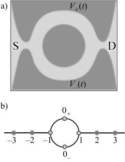
Figure 1: a) Schematic diagram of the quantum ring with a side-gate voltage $V_{\pm}(t)$ connected to source (S) and drain (D). b) Equivalent lattice model with two time-dependent site energies $\varepsilon_{\pm}(t)$ at sites labeled $0_{\pm}$ and two other sites with index $\pm 1$ attached to semi-infinite chains.

In order to study electron transport across the quantum ring, we mapped it onto a much simpler yet nontrivial lattice model, depicted in Fig. 1b). We replace the actual quantum ring by four sites of a lattice within the tight-binding approximation. Two sites ($0_{\pm}$) have time-dependent energies $\varepsilon_{\pm}(t)$ and the other two sites, labeled $\pm 1$, are connected to semi-infinite chains. Time-dependent site energies are given by $\varepsilon_{\pm}(t)=\pm 2\Delta\cos\omega t$. To avoid the profusion of free parameters, we assume a uniform transfer integral and vanishing site energies except at sites $0_{\pm}$, without loosing generality. The common value of the transfer integral will be set as the unit of energy and we take $\hbar=1$ throughout the paper.

II.1 Time-independent side-gate voltage

To gain insight into the possible occurrence of BICs in the system, we consider the time-independent case by setting $\omega=0$ for the moment. An incoming plane wave $\psi_{j}^{\mathrm{in}}(t)=\exp[i(kj-Et)]$, with energy $E=-2\cos k$ within the bands of the leads, will be partially transmitted in the form $\psi_{j}^{\mathrm{tr}}(t)=t_{0}\exp[i(kj-Et)]$. The lattice period is set as the length unit. It is a matter of simple algebra to obtain the transmission amplitude in this case

$$t_{0}=\frac{4\sin k}{4\sin k+i\left(E+4\Delta^{2}/E\right)}\ .$$ (1)

The transmission probability $T(E)=|t_{0}|^{2}$ presents a dip around the band center and vanishes at $E=0$.

In the weak coupling limit, namely $\Delta\to 0$, the transmission probability shows a Fano profile Fano61 close to the band center, $T(E)=E^{2}/\left(E^{2}+\Delta^{4}\right)$. The width of the dip scales as $\sim\Delta^{2}$. Poles of the transmission amplitude have a simple physical interpretation as the natural eigenstates of the scattering potential.Bagwell92 The poles occur at a complex energy whose real part gives the energy of the state and the imaginary part is related with its decay rate. There are four poles in the case under study. Two poles correspond to defect modes in the gap and, consequently, cannot be identified with BICs. However, the other two poles reside at the band center with an imaginary part equal to $\pm i\Delta^{2}$ when $\Delta\ll 1$. In the weak coupling limit $\Delta\to 0$ the poles correspond to truly bound states. Therefore, the Fano resonance of the transmission amplitude (1) signals the occurrence of BICs at the band center.

To get a better understanding of the nature of the BICs at the band center we also calculate the local density of states (LDOS) at sites $0_{\pm}$, $\rho_{0}(E)$. Close to the band center, the LDOS is proportional to $|\psi^{+}|^{2}+|\psi^{-}|^{2}$, where $\psi^{\pm}$ is the wave function amplitude at those sites. The LDOS is given approximately as

$$\rho_{0}(E)\sim\frac{E^{2}}{E^{2}+\Delta^{4}}+\frac{4\Delta^{2}}{E^{2}+\Delta^{4}}\ .$$ (2)

The first term is nothing but the transmission probability, vanishing at the band center. However, the second term approaches $4\pi\delta(E)$ in the limit $\Delta\to 0$, indicating the existence of a truly bound state with energy $E=0$ located at sites $0_{\pm}$.

II.2 Time-dependent side-gate voltage

We now turn to our main goal, the occurrence of BICs when the side-gate voltage depends harmonically on time. The time-dependent Schrödinger equation for the amplitudes $\psi_{j}(t)$ reads

$$i\dot{\psi}_{j}=\varepsilon_{\pm}(t)\delta_{j,0_{\pm}}\psi_{j}-\sum_{i(j)}\psi_{i(j)}\ ,$$ (3)

where the index $i(j)$ runs over the nearest-neighbor sites of $j$ and the dot indicates the derivative with respect to time. Using the Floquet formalism, the solution can be expressed in the form

$$\psi_{j}(t)=\sum_{n=-\infty}^{\infty}A_{n,j}e^{-iE_{n}t}\ ,$$ (4a)

where $$E_{n}=E+n\omega n A_{n,j}$$ and is the sideband channel index. Since we are interested in electron transmission across the ring, we take the following ansatz for the coefficients in the expansion (4a)

$$A_{n,j}=\left\{\begin{array}[]{ll}\delta_{n0}e^{ik_{n}j}+r_{n}e^{-ik_{n}j}\ ,&j\leq-1\ ,\\ f_{n}^{\pm}\ ,&j=0_{\pm}\ ,\\ t_{n}e^{ik_{n}j}\ ,&j\geq 1\ .\end{array}\right.$$ (4b)

Inserting this ansatz in (3) leads to the dispersion relation $E_{n}=-2\cos k_{n}$ where $k_{n}$ is real if $E_{n}$ lies within the band, i.e. $|E+n\omega|\leq 2$. In addition, we obtain $t_{n}=f_{n}^{+}+f_{n}^{-}=r_{n}+\delta_{n0}$, ensuring current conservation. Finally, one also gets

$$\alpha_{n}t_{n}-\frac{\Delta^{2}}{E_{n-1}}\,t_{n-2}-\frac{\Delta^{2}}{E_{n+1}}\,t_{n+2}=4i\delta_{n0}\sin k_{0}\ ,$$ (5a)

where for brevity we define

$$\alpha_{n}=4i\sin k_{n}-E_{n}-\Delta^{2}\left(\frac{1}{E_{n+1}}+\frac{1}{E_{n-1}}\right)\ .$$ (5b)

The continued fraction approach developed in Ref. Martinez01, allows us to obtain numerically the contribution of all channels to the transmission. But if the coupling of the ring to the AC side-gate voltage is weak ($\Delta\ll 1$), only the lowest order sidebands are significant. Then we keep five channels and assume that $t_{n}$ vanishes if $|n|\geq 3$. Equation (5b) implies that $t_{\pm 1}=0$ in this approximation and

$$t_{\pm 2}=\frac{\Delta^{2}}{\alpha_{\pm 2}E_{\pm 1}}\,t_{0}\ .$$ (6a)

The transmission amplitude in the elastic channel is

$$t_{0}=4i\sin k_{0}\left[\alpha_{0}-\Delta^{4}\left(\frac{1}{\alpha_{2}E_{1}^{2}}+\frac{1}{\alpha_{-2}E_{-1}^{2}}\right)\right]^{-1}\ .$$ (6b)

Once the transmission amplitudes have been calculated, we can obtain the transmission probability from the general expression

$$T_{\omega}(E)=\sum_{n}\frac{\sin k_{n}}{\sin k_{0}}\,|t_{n}|^{2}\ ,$$ (7)

where the sum runs over the propagating channels, namely those channels for which $E_{n}=E+n\omega$ lies within the band of the leads. Assuming that the sidebands are active for conduction, the transmission probability reads

$$T_{\omega}(E) =|t_{0}|^{2}\left(1+\frac{\Delta^{4}}{|\alpha_{2}|^{2}E_{1}^{2}}\,\frac{\sin k_{2}}{\sin k_{0}}\right.$$

$$\left.+\frac{\Delta^{4}}{|\alpha_{-2}|^{2}E_{-1}^{2}}\,\frac{\sin k_{-2}}{\sin k_{0}}\right)\ .$$ (8)

III Results

The five channels approximation discussed above provides a closed analytical expression for the transmission probability (8). Admittedly the resulting expression is still involved and must be evaluated numerically for the chosen parameters. We will present some simpler expressions latter, valid in the weak coupling limit, but for the moment we are interested in the closed expression (8). We assume that coupling $\Delta$ is smaller or in the order of the frequency $\omega$ hereafter. Figure 2 shows the results when the frequency is $\omega=0.5$ and $\Delta=0.1$ (recall that the amplitude is actually twice this value). The pronounced dip observed at the band center in the static case ($\omega=0$), commented above and shown in the figure, is absent if $\omega\neq 0$. Similar results can be obtained for other set of $\Delta$ and $\omega$ parameters. In fact, transmission at $E=0$ is unity and the quantum ring becomes transparent at this energy. But the most salient feature of the transmission when the side-gate voltage oscillates is the occurrence of two symmetric and narrow dips, at energies close to $\pm\omega$. Remarkably, the transmission never vanishes in the range of energy plotted in Fig. 2 and at the dips only drops at about $0.5$. Actually transmission probability vanishes but only at the band edges, as occurs in the static case too. The inset shows an enlarged view of one of the dips for two different values of the coupling $\Delta$. It is quite apparent that the minimum transmission is slightly smaller than $0.5$ and it is reached at an energy close but not exactly equal to $\omega$. In fact, transmission at $E=\omega$ is exactly equal to $0.5$ for any value of $\Delta$.

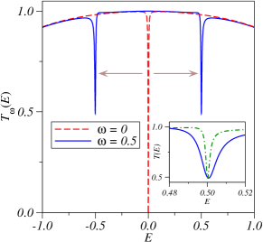
Figure 2: Transmission probability as a function of energy at $\omega=0$ (red dashed line) and $\omega=0.5$ (blue solid line) for $\Delta=0.1$. The inset shows an enlarged view of the transmission probability when $E\simeq\omega$ at $\Delta=0.01$ (green dashed line) and $\Delta=0.1$ (blue solid line) for $\omega=0.5$.

It is important to mention that we also solved numerically the general equation (5b) to obtain the transmission probability from (7), increasing the number of the sideband channels. The results were the same to those obtained within the five channels approximation, when $\Delta$ is not too large. Thus, we can confidently use this approximation in our analysis.

The transmission probability is an even function of energy. Therefore, for concreteness we now focus in the energy region close $+\omega$, when $\Delta$ is small. If $\omega$ is not large, we can take $\sin k_{\pm 2}\simeq\sin k_{0}\simeq 1$ in (8). In addition, the term containing $\alpha_{2}$ in Eqs. (6b) and (8) is negligible under these assumptions. After lengthly but straightforward algebra, the transmission probability reduces to

$$T_{\omega}(E)\simeq\frac{8(E-\omega)^{2}-\omega(E-\omega)\Delta^{2}+\Delta^{4}}{8(E-\omega)^{2}+2\Delta^{4}}\ .$$ (9a)

Since $$\omega E-\omega$$ and are not large, this expression can be further approximated by the following Fano profile

$$T_{\omega}(E)\simeq\frac{1}{2}+\frac{1}{2}\,\frac{(x-\omega/4)^{2}}{1+x^{2}}\ ,\quad x=\frac{E-\omega}{\Delta_{\mathrm{eff}}^{2}}\ .$$ (9b)

To facilitate the comparison with the static case, we have introduced an effective coupling $\Delta_{\mathrm{eff}}$ in such a way that $\Delta_{\mathrm{eff}}^{2}=\overline{\varepsilon_{\pm}^{2}(t)}=\Delta^{2}/2$, where the bar indicates the average over one time period. Notice that the Fano factor $q=-\omega/4$ becomes independent of the coupling $\Delta$. Figure 3 compares the exact results obtained from (8), for two different values of the coupling $\Delta$ and $\omega=0.5$, and the Fano profile (9b). In spite of the simplicity of the Fano profile and the assumptions we made, the agreement is remarkable in both cases.

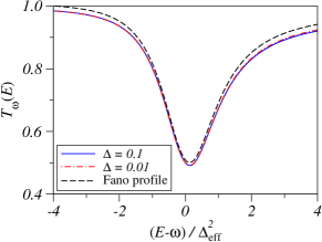
Figure 3: Transmission probability as a function of the parameter $x$ defined in (9b), for two values of $\Delta$ and $\omega=0.5$. The Fano profile is a good approximation to both curves.

In contrast to the static case, transmission at the dips remains finite when the side-gate voltage is harmonically modulated in time (see Fig. 2). Therefore, it is not clear at this stage whether the dips are due to the occurrence of BICs in the system. To answer this question we consider again the LDOS at sites $0_{\pm}$. After time-averaging over one time period, one gets

$$\overline{\rho_{0\omega}}(E) \sim\sum_{n}\left(|f_{n}^{+}|^{2}+|f_{n}^{-}|^{2}\right)$$

$$=\frac{1}{2}\sum_{n}\left(|t_{n}|^{2}+\frac{\Delta^{2}}{E_{n}^{2}}\,|t_{n+1}+t_{n-1}|^{2}\right)\ .$$

Using the five channels approximation, the LDOS close to right dip ($E\ \sim\omega$) becomes

$$\overline{\rho_{0\omega}}(E)\sim\frac{1}{2}\,T_{\omega}(E)+\frac{\Delta_{\mathrm{eff}}^{2}}{(E-\omega)^{2}+\Delta_{\mathrm{eff}}^{4}}\ ,$$ (10)

and a similar expression is obtained for the left dip ($E\ \sim-\omega$), replacing $\omega$ by $-\omega$ in (10). Therefore, in the weak coupling limit $\Delta\to 0$, the LDOS reduces to $\overline{\rho_{0\omega}}(E)\sim\delta(E+\omega)+\delta(E-\omega)$. In analogy with the static case, we claim that the two singular peaks in the LDOS at energies $\pm\omega$ are due to a new type of BICs arising by the interaction with the AC field.

IV Conclusions

In summary, we have introduced and studied a novel type of BICs in systems whose energy levels are modulated harmonically in time. To be specific, we have considered a quantum ring subjected to a side-gate voltage oscillating in time with frequency $\omega$ and studied its transport properties in a fully coherent regime. We come to the important conclusion that the BICs supported by the quantum ring in the static case survive under harmonic modulation of the side-gate voltage. The two BICs driven by the AC field have energies $\pm\omega$ and they reveal themselves in the transmission, and consequently in the low-temperature conductance, as dynamic Fano resonances. The position of the BICs inside the spectral band can be continuously tuned by varying the driving frequency and eventually they could be expelled out of the continuum when $\omega$ is larger than $2$ in units of the transfer integral, i.e. when they approaches the band edge. Similar control of the energy of static BICs have been recently demonstrated by adding weak nonlinearity to semi-infinite systems Molina12 or by varying the interaction between particles.Zhang12 However, besides the different origin of the BICs, our proposal seems to be more advantageous for the experimental validation of these exotic states. In this regard, it is still an open question to what extend electron-electron interactions would mask the effect in a real experiment. Žtiko et al. have shown that the so-called dark states in parallel double quantum dot systems are robust against interactions within a Hubbard model, at least in the Kondo regime.Zitko12 These states correspond to the BICs of our present work in the static case, which makes us confident to expect also the BICs driven by AC fields to be robust in an interacting system.

- (1) J. von Neumann and E. Wigner, Phys. Z. 30, 465 (1929).
- (2) F. H. Stillinger and D. R. Herrick, Phys. Rev. A 11, 446 (1975).
- (3) H. Friedrich and D. Wintgen, Phys. Rev. A 31, 3964 (1985).
- (4) J. M. Zhang, D. Braak, and M. Kollar, Phys. Rev. Lett. 109, 116405 (2012).
- (5) F. Capasso, C. Sirtori, J. Faist, D. L. Sivico, S.-N. G. Chu, and A. Y. Cho, Nature (London) 358, 565 (1992).
- (6) Y. Plotnik, O. Peleg, F. Dreisow, M. Heinrich, S. Nolte, A. Szameit, and M. Segev, Phys. Rev. Lett. 107, 183901 (2011).
- (7) S. Longhi, Eur. Phys. J. B 57, 45 (2007).
- (8) N. Moiseyev, Phys. Rev. Lett. 102, 167404 (2009).
- (9) E. N. Bulgakov and A. F. Sadreev, Phys. Rev. B 81, 115128 (2010).
- (10) J. U. Nöckel, Phys. Rev. B 46, 15348 (1992).
- (11) G. Ordonez, K. Na, and S. Kim, Phys. Rev. A 73, 022113 (2006).
- (12) R. Žtiko, J. Mravlje, and K. Haule, Phys. Rev. Lett. 108, 066602 (2012).
- (13) J. W. González, M. Pacheco, L. Rosales, and P. A. Orellana, Europhys. Lett. 91, 66001 (2010).
- (14) J. Munárriz, F. Domínguez-Adame, and A. V. Malyshev, Nanotech. 22, 365201 (2011).
- (15) J. Munárriz, F. Domínguez-Adame, P. A. Orellana, and A. V. Malyshev, Nanotech. 23, 205202 (2012).
- (16) U. Fano, Phys. Rev. 124, 1866 (1961).
- (17) P. F. Bagwell and R. K. Lake, Phys. Rev. B 46, 15329 (1992).
- (18) D. F. Martínez and L. E. Reichl, Phys. Rev. B 64, 245315 (2001).
- (19) M. I. Molina, A. E. Miroshnichenko, and Y. S. Kivshar, Phys. Rev. Lett. 108, 070401 (2012).